M
ASTER IN
F
INANCE
M
ASTER
’
S
F
INAL
W
ORK
D
ISSERTATION
E
VOLUTION OF
T
ANGENT
P
ORTFOLIOS
:
A
N ANALYSIS OF
THE
E
UROPEAN STOCK MARKET FROM
2000
TO
2014
M
ARIA
I
NÊS
V
ALENTE
P
EREIRA
T
RINDADE
S
ANTOS
M
ASTER IN
F
INANCE
M
ASTER
’
S
F
INAL
W
ORK
D
ISSERTATION
E
VOLUTION OF
T
ANGENT
P
ORTFOLIOS
:
A
N ANALYSIS OF
THE
E
UROPEAN STOCK MARKET FROM
2000
TO
2014
M
ARIA
I
NÊS
V
ALENTE
P
EREIRA
T
RINDADE
S
ANTOS
S
UPERVISOR
:
P
ROFESSOR
D
OCTOR
R
AQUEL
M
EDEIROS
G
ASPAR
i
Abstract
The aim of this study is to analyze the impact of four major financial shocks on European stock markets by sector. In particular, we analyze the variations in the optimal Markowitz (1952) Tangent Portfolios of European investors. These are real life portfolios, with no estimation errors. The period under analysis is from 2000 to 2014, which comprises the following shocks: (i) the 11th September, 2001; (ii) the Dot-Com
crisis, during 2000-2001; (iii) the sub-prime mortgages crisis, during 2007-2008; and (iv) the European sovereign debt crisis, during 2011. We use 16 European sector indices as underlying assets, including companies from 16 European countries. Decreased diversification in crisis periods, although milder for shorter investment horizons are some of the findings of this investigation. Also, to complement the analysis carried out in this investigation, we suggest to compose real life Tangent Portfolios using reference indices of European countries. We also propose an extension of the data-range, at least until the end of 2015, given the latest developments regarding shocks affecting Europe.
Key-Words: Diversification Across Sectors; European Sector Indices; Global Financial
ii
Acknowledgements
A Master Thesis is not completed with the authors’ write by itself. All the contributions
given throughout this writing seasons were key elements to the final work.
As so, I would like to express my sincere gratitude firstly, to my Master Thesis Supervisor Professor Doctor Raquel Medeiros Gaspar, for the unceasing support in
this final work, for her patience, motivation and vast knowledge in the subject. Her guidance assisted me in all the stages of research and writing of this investigation. I could not imagine a better mentor and supervisor.
This project would not have been possible without the help and support of my family, as well. The words to express gratefulness cannot be found, to my Parents and Brother, Rui Trindade Santos, Cristina Pereira Santos and Ruben Trindade Santos. Thank you for the strong, and constant, support, motivation and suggestions my family gave to me along this journey.
Furthermore, I would like to specially thank my Boyfriend, David De Arede Nunes, for all the help, motivation, support and extra patience during this semester. Thank you for the unslept nights, the understanding of my absence in several occasions. Thank you for helping me in every possible way.
iii
Table of Contents
Abstract ... i
Acknowledgements ... ii
List of Tables ... iv
List of Figures ... iv
List of Acronyms and Initials ... v
1. INTRODUCTION ... 6
2. LITERATURE REVIEW ... 8
2.1 A review on the impact and contagion of crises and particular shocks in financial markets between 2000 and 2014 ... 8
2.1.1 The 11th September, 2001 terrorist attacks ... 8
2.1.2 The Dot-Com crisis ... 9
2.1.3 The sub-prime mortgages crisis ... 11
2.1.4 The European sovereign debt crisis ... 12
2.2 Portfolio diversification, country and sector co-movements ... 13
3. DATA AND METHODOLOGY ... 16
3.1 Data and Periods of Analysis ... 16
3.2 Methodology ... 18
3.2.1 Portfolio Selection and Mean-Variance Theory ... 18
3.2.2 Efficient Frontiers and Tangent Portfolios ... 19
3.2.3 Investment Horizons and Rolling-Horizon procedure... 22
4. RESULTS ... 24
4.1 Sector Performance and Descriptive Statistics Analysis ... 24
4.2 Diversification across European Sectors ... 27
4.3 Tangent Portfolios ... 28
4.3.1 Risk and Return ... 28
4.3.2 Weights Distribution and Performance ... 31
5. CONCLUSIONS AND FUTURE RESEARCH ... 35
References ... 37
iv
List of Tables
TABLE 1 PERIODS DESCRIPTION –SUMMARY TABLE... 17
TABLE A-1DESCRIPTIVE STATISTICS ... 43
TABLE A-2CORRELATION MATRICES ... 44
TABLE A-3VARIANCE-COVARIANCE MATRICES ... 46
TABLE A-43-MONTHS TANGENT PORTFOLIOS’WEIGHTS AND SHARPE RATIO ... 48
TABLE A-51-YEAR TANGENT PORTFOLIOS’WEIGHTS AND SHARPE RATIO ... 49
TABLE A-65-YEARS TANGENT PORTFOLIOS’WEIGHTS AND SHARPE RATIO ... 49
List of Figures FIGURE1:EVOLUTION OF EUROPEAN SECTORS IN INDEX POINTS, FROM 2000 TO 2014 ..24
FIGURE2:EVOLUTION OF EUROPEAN SECTORS IN RETURN, FROM 2000 TO 2014 ...24
FIGURE3:3-MONTHS TANGENT PORTFOLIOS –QUARTERLY UPDATED. ...29
FIGURE4:1-YEAR PORTFOLIOS –ANNUALLY UPDATED. ...30
FIGURE5:5-YEARS PORTFOLIOS –UPDATED EVERY 5YEARS. ...30
FIGURE6:COMPOSITION OF 3-MONTHS TANGENT PORTFOLIOS ...33
FIGURE7:COMPOSITION OF 1-YEAR TANGENT PORTFOLIOS ...34
v
List of Acronyms and Initials
CESEE – Central Eastern and Southeastern Europe ECB – European Central Bank
EF – Efficient Frontier
EMU – European Monetary Union
6
1. Introduction
Crises and market financial shocks have been a hot topic in academic research throughout years. While some are worried in explaining its widespread and contagion across countries and/or markets (see, for instance, Hon et al. (2004), Dosi et al. (2006), Carmassi et al. (2009), Horta et al. (2010), Afonso et al. (2011)), other researchers are concerned with the origin and impacts that crises or particular shocks may cause in the financial markets (on the subject we suggest Howcroft (2001), Calomiris (2008), Carmassi et al. (2009), Revest and Sapio (2010), Sacco et al. (2003)).
A common aspect reported in the literature, is the globalization of trading relationships worldwide as a main driver of contagion effects. The globalization paradigm strengthened linkages across countries enabling for the rapid widespread of financial and economic shocks. Such movement is observable not only at a country level, but also at the industry level. As witnessed among academics (see Hui (2005), Patev et al. (2006), Campa and Fernandes (2006)), straight linkages across sectors are observable, for instance, culminating in a generalized and sharp fall across sectors after a down turn of internet related companies, or after the burst of the sub-prime mortgages bubble starting in the US years later.
7
greater for shorter horizons. The higher level of return for unit of additional risk incurred is obtainable updating tangent portfolios every 3-months during 2000 to 2014. In addition, we also show that European stock markets became riskier after the sub-prime crisis. Last but foremost, we find proof of milder damages of the European sovereign debt crisis in European stock markets, despite its origins in Europe. Even though, Tangent Portfolios present better performance, on average, during the sub-prime crisis period when compared to the latest.
8
2. Literature Review
The following section is divided into two main subsections providing some framework on prior literature regarding both crisis effects on financial markets.
2.1A review on the impact and contagion of crises and particular shocks in
financial markets between 2000 and 2014
In this first subsection it is presented a brief survey on topics related to each crisis under analysis. The major concerns are with their origin and further impacts on financial markets worldwide.
2.1.1 The 11th September, 2001 terrorist attacks
One of the major events that constrained European financial markets during our period of analysis, 2000-2014, was the terrorist attack of September 11th, 2001, in the US, to
the World Trade Center. The shock had a worldwide impact turning the attention of many researchers to the effects that such events can have in financial markets and international contagion. Kumar and Liu (2013) find spillover effects of terrorist attacks, particularly in countries where there is a trading partnership with the targeted country1.
The authors reinforce that the widespread of the effects is due to the increasing globalization phenomena. The analysis is made with recourse to national stock indices which performance should reflect the financial impact of those events. In accordance, Chen and Siems (2004) state that terrorist attacks do affect worldwide capital markets, yet for a brief period of time. Hon et al. (2004) test specifically for the contagion effects of the September 11th, 2001 terrorist attacks through stock prices, and find that there is a
1 The authors also refer to Arora, V., and Vamvakidis, A. (2005). How much do trading partners matter
9
higher correlation with European countries after the attacks. Moreover, investors should be able to diversify their portfolios under stability and low correlation, although this does not hold when stock markets are affected by volatility spillovers.On the investors’ behaviour, Sacco et al. (2003) find that the shock in the US impacted decision making of consumers around the world. Conversely to the ECB (2001) annual report, these presented, in the aftermaths of the attacks, an increased risk aversion and tended to invest in safer securities. In the same report, it is highlighted the major shock that such event represented in the world economy, as well as in people’s perspectives regarding the future growth under a climate of uncertainty.
2.1.2 The Dot-Com crisis
In the late 1990s internet and technological evolution marked the beginning of an era.
Both investors and analysts’ beliefs focused in this time changing process, creating a
speculative trend on internet related industries. By that time, the appearance of technology, telecommunications, and internet star-ups were steadily increasing supported by venture capitalists and biased expectations about future outcomes (Howcroft, 2001 and Revest and Sapio, 2012).
10
considered such as the typical inexperience of young managers running the start-ups. Webster (2000), Freeman and Louca (2001), and Bitmead et al. (2004) also agree that such a speculative movement that culminated in the crash of the so-called internet bubble by 2000 in the US. Conversely, Ofek and Richardson (2001) studies the behavior of internet stock prices between 1998 and 2000 in the US and demonstrates that internet stock prices were indeed overvalued and conclude that the bubble burst is potentially linked to the excess sellers in market due to expiration of lock-up agreements2. Repercussions of the Dot-Com crisis were felt at a global scale in financial
markets, mainly during 2000-2002.
Dosi et al. (2005) finds in Europe a lower presence of technological industries, when compared to US, as well as a lower propensity with respect to innovation. These findings are in accordance to those of Revest and Sapio (2012). They state that there is a low trading level of high-technology stocks, and once European technology-based small firms generally recourse to internal funds as primary source3 of funding, Europe proved
to be more resistant to the impact of the crisis. Albeit, bankruptcies, falling stock prices and decreasing capitalization were inevitable, after the bubble rush. An example of such an impact in Europe was the shutdown of the EASDAQ (European Association of Securities Dealers Automated Quotations) and the Neuer Markt4, in 2003.
2 Lockup agreements are legally binding contracts that oblige the insiders of a company to not sell the stock of that company for the next 6 months (in general). The underwriters of such agreements intend to protect the stock price against dramatic variability in the former months of trading. After the expiry date, restricted holders are allowed to sell the stock.
3 On this subject the author refers Giudici and Palcani (2000), Colombo and Grilli (2007), Scellato and
Ughetto (2010), and Carpentier et al. (2007).
4 See also Ritter, J. R. (2003). Differences between European and American IPO markets. European
Financial Management, 9(4), 421-434., Gajewski, J. F., and Gresse, C. (2006). A survey of the European
IPO market.ECMI Research Paper, (2), and Goergen, M., Khurshed, A., McCahery, J. A., and
11 2.1.3 The sub-prime mortgages crisis
The subprime crisis in the U.S. was the origin of a global financial crisis, causing strong damages in the begging of 2007 with the bankruptcy of some large and important financial institutions (e.g. Bear Stearns, Lehman Brothers). Demyanyk and Hemert (2011) shown that in turn of an increased demand for subprime mortgage-backed securities (MBS), the more was the deterioration in the quality of this increasing market. The prices at which houses were being appreciated did not reflect the effective riskiness of subprime mortgages.
Calomiris (2008) states that default risk was considerably underestimated during 2003-2007 and ascribes the responsibility to financial institutions arguing a promotion of risk taking through subsidies to leverage in housing. Conversely, Carmassi et al. (2009), as well as Kaminsky et al. (2003) and Begg (2009), argue that instability in financial markets by 2007-2008 was due to a negligent monetary policy and that banks (both in the US and in Europe) have contributed to the excessive leverage and maturity transformation. As reported in Dungey et al. (2010), one particular characteristic of the US sub-prime crisis resides in the fact that it started in the mortgages market, sprawling to the credit markets, further impacting the short-term liquidity. Blundell et al. (2008) and further Eichengreen et al. (2012), suggest that the heightened co-movement was, in
part, translated by shallow knowledge about the dimension of banks’ toxic asset
12
attention to the contagion effects due to the observation that some equity markets have fallen more than in the US, where the crash firstly occurred. Horta et al. (2010) tested the contagion of subprime crisis in European NYSE Euronext markets and find evidence of such effects. Although, Gardó and Martin (2010), comprehends that for Central Eastern and Southeastern Europe (CESEE) banks the impact is milder because of lower market penetration by structured products and lower number of specialized financial mediators. In accordance, Carmassi et al. (2009) verify that Europe also suffered from a similar real estate bubble although with a less steep decrease in the house prices.
2.1.4 The European sovereign debt crisis
Sovereign credit risk and refinancing needs are a main concern across Euro area countries, since the credit crisis of 2008. Difficulties in funding and trading markets in Europe, fueled by sovereign debt downgrades, have been the major drivers of the so-called sovereign debt crisis.
13
drivers: the type of announcement, the source country and the rating agency issuing the announcement. Afonso et al. (2011) also studies the impact both before and after rating
announcements in European Monetary Union countries’ government yield spreads arriving to the same conclusions, adding that those spillover effects are from lower to higher rated countries. Moreover, they find that negative announcements outweigh the most, especially after the Lehman Brothers collapse, as well as not anticipated announcements. Later, Ferreira and Gaspar (2013) support the evidence of these effects, specifically across PIIGS bonds. Under this context, between 2010 and 2012, it was unavoidable the need of the above mentioned countries to resort to the International Monetary Fund both to provide financial assistance and to supervise sovereign debt management, along with the ECB and European Commission, contributing to the instability among European countries.
To the best of our knowledge, little research has been done so far in what respects the impact of the European sovereign debt crisis in European stock markets. In particular, with regards to European sectors performance and to tanget portfolio decision making before, during and after such event.
2.2Portfolio diversification, country and sector co-movements
The following subsection focus on a review on portfolio diversification, particularly using either sector or country indices as underlying assets. Here added the relevance of increasingly opened economies and streghthen relationships within markets.
Investors and portfolio managers’ behaviour have been a much discussed topic. As we
suggested earlier, one of the consequences transversal to all of the shocks mentioned is
14
speculate, sometimes irrationally, believing in an upwards trend in future stock returns, or a posteriori they adjust their investment portfolios (e.g. transferring funds into safer securities) reflecting fear of further pessimistic scenarios. These matters gave rise to another line of research trying to respond to questions like (i) How do financial shocks affect portfolio construction? (ii) What are the drivers for diversification benefits? or (iii) How do linkages across sectors and/or across countries impact the ability to diversify?.
Das and Uppal (2004), analyse systemic risk effects, arising from abnormal events, in a portfolio constituted by equity indices of 5 countries (four of which European indices). Their results show that systemic risk, perceived as a direct consequence of financial
shocks, does affect the ability to diversify an investor’s portfolio. Hui (2005), emphasizes the fact that stock markets interdependence and co-movements are drivers of international diversification (portfolio diversification across countries). Facing an increase in those drivers, the ability to diversify across countries is reduced. Patev et al. (2006), with the intention of explaining Central and Eastern European equity markets co-movements, capturing market crisis impacts, also finds higher correlation and integration between these during crisis. Thus, benefits of portfolio diversification are diminished. Earlier, Meric and Meric (1997) develop a similar study for European equity markets, although with regards to the Black Monday of 1987, observing a significant decrease in international diversification due to increases in correlation between European and US equity markets after the crash.
15
concerns the increased importance of country factors over industry factors for diversification purposes5, several others observed that industry factors were overcoming
the importance of country factors. The argument for such change, according to the authors, is the increasing importance of integration and globalization. Coherent with this view, their findings suggest that as industry international integration increases results in a greater importance of industry factors. More recently, corroborating with the findings of Moerman (2008), Chou et al. (2014) document the same relationship showing that there was a reversal phenomenon in euro zone equity markets. They explain that the dominance of industry diversification was merely temporary, as the importance of country factors become equal (at times even overcome), after the crisis that started in late 2007, prevailing the evidence during the European sovereign debt crisis. Dou et al. (2014) perform a cross-region (6 world regions) and cross-sector (10 global sectors) asset allocation analysis, during 1995-2010, and conclude that under periods of high
volatility “regional returns tend to be more correlated collectively” (2014, pp. 20), and that cross-sector allocation enhance for higher Sharpe ratios and present inferior global market correlations.
Our focus and contribution from herein is to provide an analysis of European sectors evolution before, during and after the four shocks previously mentioned. Specifically, we investigate the behaviour of the optimal Markowitz (1952) Tangent Portfolio by investing exclusively in European sectors. Hence, enriching the literature we have just revised.
5 The author refers Lessard, D. R. (1974). World, national, and industry factors in equity returns. The
16
3. Data and Methodology
In this section we describe all the data and methodology used to perform the intended analysis. In Subsection 3.1 we provide information regarding the data description and timeframe of data collected. In the subsequent Subsection 3.2, the proposed methodologies are presented.
3.1 Data and Periods of Analysis
We consider 16 sector indices derived from EURO STOXX 600, in which companies are categorized under the Industry Classification Benchmark (ICB) in accordance with their major source of revenue. These are capitalization-weighted indices meaning that the components of the underlying stock are weighted in proportion to the corresponding market capitalization. Created in December 31 of 1991 with a base value of 100, these are total return indices with net dividends, i.e., dividends distributed are net of taxes and considered to be reinvested in the index, allowing for a more precise analysis of the index performance. In particular, we consider the following sectors: automobile and parts, oil and gas, financial services, construction and materials, health care, chemicals, telecommunications, personal and household goods, media, industry goods and services, banks, retail, food and beverage, insurance, travel and leisure, and technology. Our indices include companies from Austria, Belgium, Denmark, Finland, France, Germany, Ireland, Italy, Luxembourg, Netherlands, Norway, Portugal, Spain, Sweden, Switzerland and United Kingdom. For each of these we collect historical daily values since the December 30th of 1999 until the May 6th of 2015.
17
and 5-years), we decided to use EURIBOR and the German Bund. EURIBOR are reference rates for periods up to 1 year, devoted in euro interbank market for unsecured lending operations. Thus, we collect daily historical data on EURIBOR 3 months and 12 months rates. The same procedure for the longer maturity portfolios is carried out, although considering the 5-year German Bund yield, frequently used as European riskless benchmark, in the presence of long-term investments.6
In Table 1 we present a summary description of the 7 periods stablished, as well as their corresponding dates.
TABLE 1
PERIODS DESCRIPTION –SUMMARY TABLE
Period Dates Description
Period 1. – Non-Crisis From January of 2000 to August
of 2001.
Marks the beginning of our sample range until the 11 days
preceding the 1st shock
considered in our analysis.
Period 2. – Crisis From September of 2001 to
March of 2003.
Comprehends both effects of the 11th September, 2001 terrorist attacks to the World Trade Centre in the US and the Dot.Com crisis in Europe.
Period 3. – Non-Crisis From April of 2003 to
December of 2006.
Period between the Dot.Com
crisis and the Sub-prime
mortgages crisis.
Period 4. – Crisis From January of 2007 to June of
2009.
During the Sub-prime
mortgages crisis.
Period 5. – Non-Crisis From July of 2009 to December
of 2010.
Corresponds to an upturn of European stock markets after the Sub-prime mortgages crisis and before the European Sovereign Debt crisis.
Period 6. – Crisis From January of 2011 to
December of 2011.
Elapse of the European
Sovereign Debt crisis.
Period 7. – Non-Crisis From January of 2012 to
December of 2014.
Post European Sovereign Debt crisis.
18
We divide our sample into 7 periods. These periods are created both based upon the literature review on the crises, and on the analysis of our sector indices performance throughout the our data range (2000-2014). Similarly to what Dungey et al. (2010) have done, this division allows us to define crisis and non-crisis moments. On the other hand, it also provides ease of interpretation when it comes to results.
3.2 Methodology
At first, in Subsections 3.2.1, 3.2.2, and 3.2.3, we go through the Mean-Variance and tangent portfolio backgrounds and modulation. Secondly, in Subsection 3.2.4, we add information on the procedure carried out to perform our analysis. Finally, in Subsection 3.2.5, we present 7 periods we built from our sample in order to locate crisis and non-crisis moments.
3.2.1 Portfolio Selection and Mean-Variance Theory
Back in 1952, Markowitz develops his first approach with regards to portfolio selection. The booster of the well-known Modern Portfolio Theory primarily starts by defining two stages that optimal portfolio selection should follow: the first beginning with observation and experience, ending with expectations about future performance of available assets; the second handles with relevant expectations on future performance and settles with the choice of the portfolio.
19
Markowitz clarifies that holding a portfolio comprising inversely correlated assets will
generate benefits to the investor as he will be able to disseminate assets’ specific risk.
Hence, the efficient frontier is the set of efficient mean-variance portfolios that combine the maximum expected return incurring in the lowest levels of risk.
Further on, Markowitz (1956), Markowitz (1959), Markowitz and Levy (1979) and Markowitz (1991), proceed the debate extending the original setup. More recently, Markowitz (2014) elucidates several assumptions made in the author’s prior frameworks namely that he never assumed that return distributions are Gaussian rather than t-student approximations for instance, as proven in Markowitz and Usmen (1996a, 1996b), or that the utility function of an investor is quadratic.
3.2.2 Efficient Frontiers and Tangent Portfolios
In a world where there is a riskless asset at which an investor can either borrow or lend, as considered in Tobin (1958), it is possible to obtain the investment opportunity set by combining risky assets, or risky assets with another which is risk free. With the inclusion of a riskless asset, the efficient frontier becomes a straight line with slope given by 𝜃 = (𝑅̅𝑝− 𝑅𝑓)
σ𝑝 , where 𝑅𝑓 represents the considered riskless return. In Sharpe
(1966), the author studies the performance of mean-variance modeled portfolios using mutual funds, by comparing two measures: Treynor and Sharpe ratios. He concludes
20
portfolio. Additionally, for the purpose of this investigation, it is important to convey that while Treynor’s measure relies on an equilibrium model7, the Sharpe ratio only
depends on the premium per unit of aditional incurred measured by expected returns and volatilities. The portfolio with the maximum Sharpe ratio is known as tangent portfolio.
The practice carried out to build our tangent portfolios is as follows. To begin with, we take the Neperian logarithm of the fraction between the value of the index, ‘’I’’, in
moment ‘’t’’ and its value in the previous time instant ‘’t-1’’, in order to obtain the realized returns on moment ‘’t’’, 𝑟𝑖,𝑡:
𝑟𝑖,𝑡 = ln (𝐼𝑡−1𝐼𝑡 ). (1)
We then take the mean returns doing the arithmetic average and annualize them. Given that we are using daily returns, it is relevant to clarify that we annualize the average returns by multiplying its value by the number of trading days in a year ‘’N’’ of the timeframe to be considered (we consider 𝑁 = 252 for computational simplicity):
𝑟̅𝑡 = (∑ 𝑟𝑖,𝑡
𝑁 𝑡=1
𝑁 ) ∗ 𝑁. (2)
To calculate the annualized variance of the returns, we shall start by calculating their standard deviation,σ𝑖 , which is nothing more than the squared root of the variance:
σ𝑖 = √∑ (𝑟𝑖,𝑡− 𝑟̅𝑖)
2 𝑁
𝑖=1
𝑁−1 ∗ √𝑁. (3)
7 𝑇𝑌 = 𝑅̅𝑝− 𝑅𝑓
𝛽𝑝 , where 𝛽𝑝 reflects the market risk under the assumptions of the Capital Asset Pricing
21
Covariance matrix is obtained through the primary formula for the covariance between 2 assets, for instance, index “l” and index “k”:
σ𝑙𝑘 = ∑𝑗=1𝑁 (𝑟𝑙,𝑗−𝑟̅𝑙𝑁−1 )(𝑟𝑘,𝑗−𝑟̅𝑘). (4)
Finally, portfolios’ expected returns, 𝑅̅𝑝, and corresponding risk, denoted by their standard-deviation, σ𝑝 , are given by:
𝑅̅𝑝 = ∑𝑁𝑖=1𝐸(𝑋𝑖𝑅̅𝑖) (5)
and
σ𝑝 = √∑ (𝑋𝑗2σ𝑗2) + ∑ ∑𝑘=1𝑁 (𝑋𝑗𝑋𝑘σ𝑗𝑘 )
𝑘≠𝑗 .
𝑁 𝑗=1 𝑁
𝑗=1 (6)
Nevertheless, the weights, 𝑋𝑖 of a tangent portfolio, are the result of the optimization carried out to obtain our optimal portfolios. Hence, we have set the objective function to maximize the Sharpe ratio of the portfolio, 𝜃 = (𝑅̅𝑝− 𝑅𝑓)
σ𝑝 , where 𝑅𝑓 represents the
considered riskless asset. Moreover, we subject the objective to the constraints:
∑𝑁𝑖=1𝑋𝑖 = 1, i.e., the sum of the portfolios’ weights should equal 1; 𝑋𝑖 ≥ 0, reflecting
that on each index one should invest only amounts held, as we do not allow for short positions8. This last restriction is due to the fact that, for the majority of the countries
considered in the present study short-selling is allowed under strict restrictions regulated by the European Securities and Markets Authority (ESMA)9. Among others, to take a
short position an investor should do it through a financial institution that assumes
8All formulas using, follow Elton et al.’s (2014) notation.
22
responsibility for the asset liquidation, thus, the investor should hold assets that are worth at least the value of its position.
3.2.3 Investment Horizons and Rolling-Horizon procedure
We aim to analyze weights distribution of tangent portfolios over time across sectors. Changes in weights along time are key to understand market behavior and investors preferences, in the search for the tangent decision.
This study considers different investment horizons: (i) 3-months portfolios, which are updated every 3 months; (ii) 12-months portfolios, updated every year; and (iii) 5-year portfolios, updated every 5 years. To be able to constitute portfolios covering the intended investment horizons, over our large range of historical daily returns, a rolling-horizon procedure was applied. The rolling-horizon is commonly performed among
existing literature concerning portfolio performance10, as follows. However, for this
investigation we perform the rolling-horizon procedure building windows with 3 months, 1 and 5 years of daily historical data. For each of these, we update our optimal portfolios every 3-months, 12-months and 5-year. The first tangent portfolio comprising investment horizons of three months, is built in the 2nd of January of 2000, with recorse
to returns realized in the following 3 months. By ‘’rolling’’ one time instant window (3 moths in this case), we are able to constitute the second portfolio, updated in the 3rd of
April of 2000. The same procedure is followed until the period of analysis is complete. Similarly, we adopt the same steps to construct the 12-months and 5-years portfolios. As a result, we obtain 61 real life portfolios with an investment horizon of 3 months, 15 with an investment horizon of 1 year, and 3 with an investment horizon of 5 years. Such
10 See, for instance, Ben-Tal et al. (2000), Pinar (2007), DeMiguel and Nogales (2009), DeMiguel et al.
23
24
4. Results
4.1Sector Performance and Descriptive Statistics Analysis
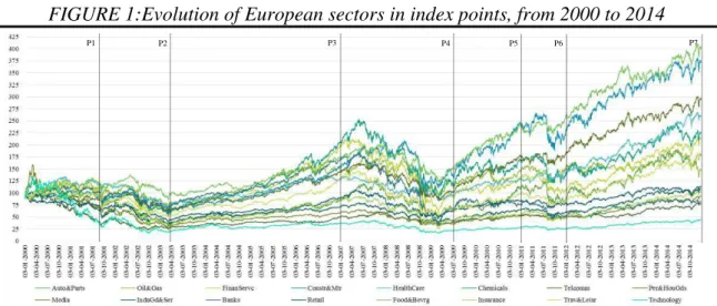
The following figures provide an overview of the European sectors evolution throughout crisis and non crisis periods. From direct examination of the graphs we are able to observe volatility changes in times of market instability. Thus, they may shed light of the persistence/duration about the impact of each shock under analysis on European stock markets.
FIGURE 1:Evolution of European sectors in index points, from 2000 to 2014
Figure 1 plots the evolution of European sectors used to perform our analysis. These are in index points, with a base of 100 in the first trading day of January, 2000, which marks the beginning of our data range. The vertical dashed lines determine the end of each period of crisis and non-crisis.
FIGURE 2: Evolution of European sectors in return, from 2000 to 2014
Figure 2 plots the evolution of European sectors used to perform our analysis. These are logarithmic returns, since the first trading day, in January of 2000, until the end of our data range, in December of 2014. The vertical dashed lines determine the end of each period of crisis and non-crisis.
P1 P2 P3 P4 P5 P6 P7
25
It is observable the presence of higher volatility for periods 1 and 2 when compared to period 3, although it is slightly higher in the second half of 2002. In Period 4, it is by the end of 2008 that European stock markets resent the most. The beginning of Period 5, which comprehends the first half of 2009, there are still traces of the instability felt in the preceding period. Eventhough, it is after the second half of 2009 that stock markets in Europe reflect more stability. European sector indices’ volatility remains low until mid-2011, in period 6, followed by little turmoil until the end of 2011. Period 7 appears to be the most stable.
Table A- 1, in appendix, allows for a deeper analysis of the above described results, enabling comparisons both across sectors and across the stablished periods. In general, we can observe a diminishing trend for the mean values realized in crisis periods in comparison to those observed in non-crisis periods, as well as higher levels of standard-deviation, across all sectors under analysis. Particularly, Periods 2 and 4 register the highest levels of standard-deviation. Nonetheless, Period 5 is also noticeable as the non-crisis period that presents higher volatility, reflecting perhaps the lack of confidence throughout the period following the sub-prime mortgages crisis.
26
6 caused less impact in European stock markets suggests that its origin in fixed income markets did not spread at a large scale to stock markets. Yet, the sectors that contributed the most for the instability felt in this period were auto and parts, banks and insurance. It is transversal through all periods high volatility for the auto and parts sector, although it has not been a target factor among researchers interests. We shall imply that it is a very volatile sector that reacts greatly to particular shocks in markets, albeit we are not able to argue about what specific events contribute for such outliers.
At this stage we are able to draw some relevant notes. By analysing the evolution of our sector indices, as well as their corresponding descriptive statistics, between 2000 and 2014, it is evident that the shocks caused by the 11th September of 2001 and the internet
bubble crisis were the most persistent, followed by the sub-prime crisis that constrained European stock markets for a period of approximatly one year and a half, and that the European sovereign debt crisis was the shock that least damaged European stock markets. Furthermore, there seems to exist a delay between the reaction of European stock markets to the Dot.com crisis, compared to that of US stock markets. As reported in the literature, US stock markets started to fall in the early 2000s, while in Europe, despite the instability felt since that date, it is in the aftermaths of the 11th September of
27
volatile sector throughout our sample period is food and beverage, followed by the health and care sectors.
4.2Diversification across European Sectors
By analysing both correlation and variance-covariance matrices across periods between our selected sectors, which shall be found in appendix, Table A- 2 and Table A- 3 correspondingly, the overall conclusion is that these present increased values in crisis moments.
In what respects correlation (see appendix, Table A- 2), which may translate the potencial contagion across sectors of one determined market movement, almost all sectors show positive and statistically significant correlation throughout our data range.
Although there is, in general, an increase in correlations during crisis periods, it is observable a general increase in the base values even in less contorbated periods. As previously presented in our literature review, such fact is coherent with an increasing opening and narrow relations between economies, as well as a subsequent increased dependence between sectors. The industry specialization of European economies bring out the necessity of strenghthen trading relationships with each other.
28
With regards to the variances and covariances, it is possible to understand how did the riskiness of the analysed assets evolved, as well as to comprehend wheather it would be possible to diversify across sectors in Europe.
As expected, almost all assets under analysis present positive covariance every period. The fact that European economies have become more and more linked, driven such results. As time passes by, markets show up riskier and, although there are still clear differences between crisis and non-crisis moments, the gap became lower after the sub-prime crisis. Also argued in the literature, people beliefs and confidence were deteriorating when confronted with the dramatic impact that events located in opposite sides of the world would cause in their own economies.
As a further remark, the figures discussed in this subsection bring out the difficulty to diversify across sectors in Europe. We address this topic further on, in Subsection 4.3.2.
4.3Tangent Portfolios
Moving on to the Tangent Portfolios, we dedicate the following subsections to an analysis of their behaviour. Specifically, we analyse the results which, from an
insvestor’s perspective, one would be able to reach under the circumstances priorly described.
4.3.1 Risk and Return
29
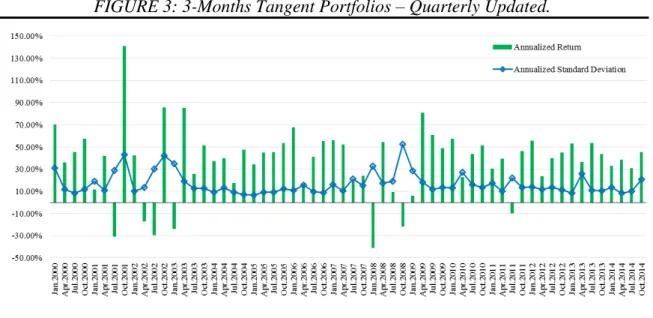
In fact, we observe in Figure 2 that one holding a three months portfolio for the period between 2000 and 1014, would incur in higher losses in moments of crisis, but would also be able to benefit from higher returns in times of recovery. When compared to longer investment horizons (both 1-year and 5-years, see figures 3 and 4), the risk oscilates within the same values while the gap between these and returns obtained decreases.
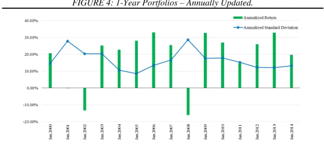
Thus, on average, for an investment horizon of three months the investor would have been able to receive a return of 37.77% facing a risk of 16.82%, which is the best possible outcome attainable for a tanget portfolio investor indifferent about the investment horizon. Hence, for investment horizons of one year and five years, the average return would decrease to 18.55% and 10.24%, respectively, with average risks of 16.61% and 16.21%.
FIGURE 3: 3-Months Tangent Portfolios – Quarterly Updated.
30
FIGURE 4: 1-Year Portfolios – Annually Updated.
The figure shows the annualized return and standard deviation of each portfolio with an investment horizon of 1 year. Reflected dates refer to the starting date of each portfolio. All the updates are considered to be made in the first trading day of every 1-year portfolio.
FIGURE 5: 5-Years Portfolios – Updated every 5 Years.
The figure shows the annualized return and standard deviation of each portfolio with an investment horizon of 5 years. Reflected dates refer to the starting date of each portfolio.All the updates are considered to be made in the first trading day of every 5-years portfolio.
31 4.3.2 Weights Distribution and Performance
Along with the figures analysed in section 4.2 and in the second part of our literature review, results flow into one major conclusion: decreasing ability to diversify across-sectors under financial market shocks and as time passes by.
The evidence points out increased difficulty to diversify across sectors in Europe, due to increasingly positive co-movements and correlations among sectors (see appendix Tables A- 4, A- 5 and A- 6 conjoined with the results from the previous subsection). When investing under financial turmoil, diversification benefits are reduced. The ability to diversify a tanget portfolio across European sectors depends on whether the portfolio is built under crisis or non-crisis moments. Hence, in periods of financial turmoil, there is a tendency to concentrate the investments in safer securities (those with lower volatility levels over time). Thus, in what respects economic/financial recovery and stability periods, it is increased the ability to diversify across-sectors allowing to obtain higher levels of return for additional unit of risk incurred. Furthermore, benefits from diversification are also decreasing with an extension of the investment horizon. As priorly discussed, on average, the risk obtained in each investment horizon is similar although corresponding to lower returns as the investment horizon expands.
32
for the following three months. The best performance would be achieved in October of 2004 (Period 3), holding 100% of the portfolio in the sector of Financial Services, reaching a sharpe ratio of 6.47. In the case of one-year portfolios, the worse performance portfolio (sharpe ratio of -0.85), yet the best tangent alternative so far, would be reached with 100% invested in Food&Beverage by January of 2002 (Period 2). The greatest performance with a sharpe ratio of 2.99, for the same investment horizon, is achieved by investing as of January, 2005 (Period 3): 26% in Financial Services, 25% in Construction&Materials, 29% in Heath Care, 5% in Personal&Household Goods and 15% in Food&Beverage. Finally, concerning five-years investment horizons, by January of 200011 the best possible outcome obtainable
would be to invest 100% in Food&Beverage for the subsequent 5 years (sharpe ratio of -0.09), while investing 63% in Health Care, 23% in Food&Beverage and 15% in Travel&Leisure in January of 2010 it would allow for a sharpe ratio of 1.19, which is the highest among all three portfolios. By looking at these numbers, it is clear that one would be able to achieve higher performance levels in non-crisis periods. Such fact is more evident for portfolios comprising 3-Months investment horizons.
33
The following figures set an example of the changes in our realized Tangent Portfolios’ composition throughout the analized period, 2000-2014.
FIGURE 6: Composition of 3-Months Tangent Portfolios
July.2000 – Period 1 January.2002 – Period 2 October.2004 – Period 3
April.2009 – Period 4 July.2009 – Period 5 April.2011 – Period 6
January.2013 – Period 7
Legend:
The figures presented have been selected based upon the highest sharpe ratio realized each period for real life Tangent Portfolios
34
FIGURE 7: Composition of 1-Year Tangent Portfolios
January.2000 – Period 1 January.2005 – Period 3 January.2013 – Period 7
Legend:
The figures presented set an example of the best performance real life Tangent Portfolios for a 1-Year investment horizon.
FIGURE 8: Composition of 5-Years Tangent Portfolios
January.2000(a) January.2005(b) January.2010(c)
Legend:
(a) Portfolio that comprises Periods 1. and 2., and the first two years of Period 3. (b) Portfolio that comprises the last two years of
Period 3. It also includes Period 4. as well as the first half year of Period 5.(c) Portfolio that includes the last year of Period 5., and
covers Periods 6. and 7. fully.
35
5. Conclusions and Future Research
The main objective of the present investigation is to understand how would the optimal Markowitz (1952) real life Tangent Portfolios composed by European sector indices behave during 2000 to 2014. In order to undertake this analysis, we decided to build portfolios comprising 3 investment horizons: (i) 3-months; (ii) 1-year; (iii) 5-years; using a rolling-horizon procedure, without estimation errors, provided the use of realized returns. Throughout the analysed period, there were four major financial shocks felt at a global scale: (i) the 11th September, 2001; (ii) the Dot-Com crisis, during
2000-2001; (iii) the sub-prime mortgages crisis, during 2007-2008; and (iv) the European sovereign debt crisis, during 2011. As so, it enabled not only for the understanding of Tangent Portfolio variations, but also for the comprehension of the evolution of
European sectors both before and after dramatic financial crisis and/or shocks.
As a result, we’ve shown that, from 2000 to 2014, European stock markets became
36
37
References
Afonso, A., Furceri, D., and Gomes, P. (2012). Sovereign credit ratings and financial markets linkages: application to European data. Journal of International Money and Finance, 31(3), 606-638.
Arezki, R., Candelon, B., and Sy, A. N. R. (2011). Sovereign rating news and financial markets spillovers: Evidence from the European debt crisis. IMF working papers, 1-27.
Arora, V., and Vamvakidis, A. (2005). How much do trading partners matter for economic growth?. IMF staff papers, 24-40.
Begg, I. (2009). Regulation and Supervision of Financial Intermediaries in the EU: The Aftermath of the Financial Crisis*. JCMS: Journal of Common Market Studies, 47(5), 1107-1128.
Bekaert, G., Ehrmann, M., Fratzscher, M., and Mehl, A. J. (2011). Global crises and equity market contagion (Working Paper No. 17121). National Bureau of Economic Research Working Paper.
Ben-Tal, A., Margalit, T., and Nemirovski, A. (2000). Robust modeling of multi-stage portfolio problems. InHigh performance optimization, 303-328. Springer US. Bitmead, A., Durand, R. B., and Ng, H. G. (2004). Bubblelepsy: the behavioral
wellspring of the internet stock phenomenon. The Journal of Behavioral Finance, 5(3), 154-169.
Blundell-Wignall, A., and Atkinson, P. (2008). The subprime crisis: Causal distortions and regulatory reform. Lessons from the Financial Turmoil of 2007 and 2008.
Calomiris, C. W. (2008). The subprime turmoil: What’s old, what’s new, and what’s
next. Maintaining Stability in a Changing Financial System, 21-23.
38
Carmassi, J., Gros, D., and Micossi, S. (2009). The Global Financial Crisis: Causes and Cures*. JCMS: Journal of Common Market Studies, 47(5), 977-996.
Carpentier, C., Liotard, I., and Revest, V. (2007). La promotion des firmes françaises de biotechnologie. Le rôle de la propriété intellectuelle et de la finance. Revue d'économie industrielle, (120), 79-94.
Chen, A. H., and Siems, T. F. (2004). The effects of terrorism on global capital markets. European journal of political economy, 20(2), 349-366.
Chou, H. I., Zhao, J., and Suardi, S. (2014). Factor reversal in the euro zone stock returns: Evidence from the crisis period. Journal of International Financial Markets, Institutions and Money, 33, 28-55.
Colombo, M. G., and Grilli, L. (2007). Funding gaps? Access to bank loans by high-tech start-ups. Small Business Economics, 29(1-2), 25-46.
Das, S. R., and Uppal, R. (2004). Systemic risk and international portfolio choice. The Journal of Finance, 59(6), 2809-2834.
De Santis, R. A. (2012). The Euro area sovereign debt crisis: safe haven, credit rating agencies and the spread of the fever from Greece, Ireland and Portugal.
DeMiguel, V., and Nogales, F. J. (2009). Portfolio selection with robust estimation. Operations Research, 57(3), 560-577.
DeMiguel, V., Garlappi, L., Nogales, F. J., and Uppal, R. (2009). A generalized approach to portfolio optimization: Improving performance by constraining portfolio norms. Management Science, 55(5), 798-812.
DeMiguel, V., Plyakha, Y., Uppal, R., and Vilkov, G. (2013). Improving portfolio selection using option-implied volatility and skewness. Journal of Financial and Quantitative Analysis, 48(06), 1813-1845.
39
Dosi, G., Llerena, P., and Sylos Labini, M. (2005). Science-technology-industry links and the" European paradox": Some notes on the dynamics of scientific and technological research in Europe (Working Paper No. 02). LEM Working Paper series.
Dou, P. Y., Gallagher, D. R., Schneider, D., and Walter, T. S. (2014). Cross‐region and cross‐sector asset allocation with regimes. Accounting & Finance, 54(3), 809-846.
Dungey, M., Fry, R., Martin, V. L., Tang, C., and González-Hermosillo, B. (2010). Are Financial Crises Alike?. IMF Working Papers, 1-58.
ECB (2001), Annual Report. European Central Bank, Germany. Available at: https://www.ecb.europa.eu/pub/pdf/annrep/ar2001en.pdf?3becbb79ba303bda5c9 8074b60787475.
Eichengreen, B., Mody, A., Nedeljkovic, M., and Sarno, L. (2012). How the subprime crisis went global: evidence from bank credit default swap spreads. Journal of International Money and Finance, 31(5), 1299-1318.
Elton, E. J., Gruber, M. J., Brown, S. J., and Goetzmann, W. N. (2014). Modern Portfolio Theory and Investment Analysis, 9th Ed. Hoboken, NJ, USA: John Wiley & Sons.
ESMA (2015). Retrieved in June 8, 2015 from the website:
http://www.esma.europa.eu/page/Short-selling.
Ferreira, S. and R.M. Gaspar (2013). Spillovers across PIIGS bonds. ISEG Working Paper.
Fontana, A., and Scheicher, M. (2010). An analysis of euro area sovereign CDS and their relation with government bonds.
40
Gajewski, J. F., and Gresse, C. (2006). A survey of the European IPO market. ECMI Research Paper, (2).
Gardó, S., and Martin, R. (2010). The impact of the global economic and financial crisis on central, eastern and south-eastern Europe: A stock-taking exercise. ECB Occasional paper, (114).
Giudici, G., and Paleari, S. (2000). The provision of finance to innovation: a survey conducted among Italian technology-based small firms. Small Business Economics, 14(1), 37-53.
Goergen, M., Khurshed, A., McCahery, J. A., and Renneboog, L. (2003). The rise and fall of the European New Markets: On the short and long-run performance of high-tech initial public offerings. ECGI-Finance Working Paper, (27).
Hon, M. T., Strauss, J., and Yong, S. K. (2004). Contagion in financial markets after September 11: myth or reality?. Journal of Financial Research, 27(1), 95-114. Horta, P., Mendes, C., and Vieira, I. (2010). Contagion effects of the subprime crisis in
the European NYSE Euronext markets. Portuguese Economic Journal, 9(2), 115-140.
Howcroft, D. (2001). After the goldrush: deconstructing the myths of the dot. com market. Journal of Information Technology, 16(4), 195-204.
Hui, T. K. (2005). Portfolio diversification: a factor analysis approach. Applied Financial Economics, 15(12), 821-834.
Kaminsky, G. L., Reinhart, C., and Vegh, C. A. (2003). The unholy trinity of financial contagion (Working Paper No. 10061). National Bureau of Economic Research Working Paper.
Kumar, S., and Liu, J. (2013). Impact of terrorism on international stock markets. Journal of Applied Business and Economics, 14(4), 42-60.
41
Levy, H., and Markowitz, H. M. (1979). Approximating expected utility by a function of mean and variance. The American Economic Review, 308-317.
Markowitz, H. (1952). Portfolio selection*. The journal of finance, 7(1), 77-91.
Markowitz, H. (1959). Portfolio selection: efficient diversification of investments. Cowies Foundation Monograph, (16).
Markowitz, H. M. (1991). Foundations of portfolio theory. Journal of Finance, 469-477.
Markowitz, H. M., and Usmen, N. (1996). The likelihood of various stock market return distributions, Part 1: Principles of inference. Journal of Risk and Uncertainty, 13(3), 207-219.
Markowitz, H. M., and Usmen, N. (1996). The likelihood of various stock market return distributions, Part 2: Empirical results. Journal of Risk and Uncertainty, 13(3), 221-247.
Meric, I., and Meric, G. (1997). Co-movements of European equity markets before and after the 1987 crash. Multinational Finance Journal, 1(2), 137-152.
Moerman, G. A. (2008). Diversification in euro area stock markets: Country versus industry. Journal of International Money and Finance, 27(7), 1122-1134.
Ofek, E., and Richardson, M. (2001). Dotcom mania: The rise and fall of internet stock prices (Working Paper No. 8630). National Bureau of Economic Research Working Paper.
Patev, P., Kanaryan, N., and Lyroudi, K. (2006). Stock market crises and portfolio diversification in Central and Eastern Europe. Managerial Finance, 32(5), 415-432.
Pınar, M. Ç. (2007). Robust scenario optimization based on downside-risk measure for multi-period portfolio selection. OR Spectrum, 29(2), 295-309.
42
Ritter, J. R. (2003). Differences between European and American IPO Markets. European Financial Management, 9(4), 421-434.
Sacco, K., Galletto, V., and Blanzieri, E. (2003). How has the 9/11 terrorist attack influenced decision making?. Applied Cognitive Psychology, 17(9), 1113-1127. Scellato, G., and Ughetto, E. (2010). The Basel II reform and the provision of finance
for R & D activities in SMEs: An analysis of a sample of Italian companies. International Small Business Journal, 28(1), 65-89.
Sharpe, W. F. (1966). Mutual fund performance. Journal of business, 39(1), 119-138. Tobin, J. (1958). Liquidity preference as behavior towards risk. The Review of
Economic Studies, 65-86.
43
Appendix
TABLE A-1
DESCRIPTIVE STATISTICS
.
A&P Oil&Gas FinSrvc C&M HealthCare Chemicals Telcomm P&HGds Media IGds&Srvc Banks Retail F&B Insur T&L Tech
Mean 0,02% 0,02% 0,01% -0,01% 0,03% -0,02% -0,22% -0,04% -0,09% -0,11% 0,00% -0,08% 0,04% -0,02% -0,02% -0,23%
Stand. Error 0,10% 0,07% 0,06% 0,05% 0,06% 0,05% 0,12% 0,07% 0,11% 0,06% 0,06% 0,05% 0,05% 0,06% 0,06% 0,16%
Stand. Dev. 2,14% 1,49% 1,15% 1,00% 1,22% 1,11% 2,52% 1,37% 2,27% 1,16% 1,21% 0,96% 1,06% 1,16% 1,21% 3,28%
Min. -4,56% -5,38% -5,06% -5,23% -5,28% -5,11% -7,57% -5,61% -8,08% -3,92% -4,48% -4,56% -5,73% -7,26% -3,94% -12,22%
Max. 39,43% 6,80% 4,44% 3,06% 3,00% 4,42% 7,63% 3,37% 9,02% 3,03% 4,11% 2,69% 5,96% 4,39% 3,57% 10,76%
No. Of days 426 426 426 426 426 426 426 426 426 426 426 426 426 426 426 426
Mean -0,19% -0,09% -0,16% -0,11% -0,12% -0,12% -0,09% -0,08% -0,21% -0,14% -0,10% -0,14% -0,06% -0,28% -0,15% -0,17%
Stand. Error 0,13% 0,11% 0,10% 0,08% 0,09% 0,10% 0,13% 0,09% 0,12% 0,13% 0,11% 0,08% 0,07% 0,15% 0,10% 0,17%
Stand. Dev. 2,67% 2,12% 2,06% 1,51% 1,73% 1,90% 2,53% 1,74% 2,43% 2,60% 2,10% 1,66% 1,37% 2,95% 2,05% 3,32%
Min. -28,94% -7,45% -9,53% -5,39% -6,32% -6,16% -8,16% -7,89% -8,43% -8,24% -8,99% -6,78% -4,85% -12,05% -12,59% -7,20%
Max. 8,17% 5,74% 6,27% 4,67% 6,55% 8,60% 7,57% 5,63% 7,79% 24,37% 7,46% 5,51% 6,19% 9,76% 5,75% 10,35%
No. Of days 399 399 399 399 399 399 399 399 399 399 399 399 399 399 399 399
Mean 0,09% 0,07% 0,13% 0,13% 0,06% 0,10% 0,06% 0,09% 0,07% 0,07% 0,09% 0,08% 0,06% 0,11% 0,10% 0,07%
Stand. Error 0,04% 0,03% 0,03% 0,03% 0,03% 0,03% 0,03% 0,03% 0,03% 0,03% 0,03% 0,02% 0,02% 0,04% 0,03% 0,05%
Stand. Dev. 1,20% 1,02% 0,85% 0,90% 0,82% 0,96% 0,94% 0,82% 0,99% 0,99% 0,85% 0,77% 0,68% 1,16% 0,92% 1,46%
Min. -4,47% -3,52% -5,19% -5,17% -3,52% -5,19% -4,58% -3,28% -4,11% -4,11% -3,20% -3,08% -4,93% -5,50% -4,67% -8,65%
Max. 5,84% 3,61% 4,01% 3,81% 3,23% 4,81% 3,84% 3,75% 4,81% 4,81% 3,45% 2,44% 2,09% 6,50% 4,90% 7,63%
No. Of days 965 965 965 965 965 965 965 965 965 965 965 965 965 965 965 965
Mean -0,04% -0,04% -0,12% -0,08% -0,05% -0,02% -0,04% -0,05% -0,08% -0,08% -0,15% -0,06% -0,02% -0,11% -0,11% -0,08%
Stand. Error 0,14% 0,09% 0,09% 0,09% 0,05% 0,08% 0,07% 0,06% 0,07% 0,07% 0,11% 0,07% 0,05% 0,10% 0,08% 0,08%
Stand. Dev. 3,56% 2,20% 2,32% 2,31% 1,36% 1,92% 1,69% 1,59% 1,65% 1,65% 2,77% 1,74% 1,38% 2,65% 2,00% 2,11%
Min. -35,43% -10,04% -10,32% -10,30% -6,82% -8,05% -9,44% -7,07% -7,66% -7,66% -10,90% -7,42% -6,02% -12,18% -7,49% -9,97%
Max. 40,82% 11,86% 12,31% 11,19% 8,60% 11,62% 9,66% 8,96% 9,51% 9,51% 16,09% 7,29% 7,27% 13,42% 8,93% 8,56%
No. Of days 639 639 639 639 639 639 639 639 639 639 639 639 639 639 639 639
Mean 0,12% 0,05% 0,08% 0,08% 0,08% 0,15% 0,07% 0,14% 0,10% 0,10% 0,03% 0,07% 0,12% 0,07% 0,11% 0,07%
Stand. Error 0,10% 0,06% 0,07% 0,08% 0,04% 0,07% 0,05% 0,06% 0,06% 0,06% 0,09% 0,05% 0,05% 0,08% 0,06% 0,06%
Stand. Dev. 1,89% 1,27% 1,34% 1,61% 0,80% 1,30% 1,05% 1,10% 1,14% 1,14% 1,82% 1,02% 0,92% 1,53% 1,25% 1,25%
Min. -5,39% -3,94% -4,97% -4,40% -3,51% -4,19% -4,28% -4,16% -4,98% -4,98% -5,60% -4,35% -3,76% -4,42% -5,21% -4,86%
Max. 6,41% 4,72% 6,89% 8,41% 2,99% 5,48% 6,77% 5,60% 5,75% 5,75% 13,49% 5,41% 4,00% 10,38% 6,00% 4,75%
No. Of days 389 389 389 389 389 389 389 389 389 389 389 389 389 389 389 389
Mean -0,10% 0,02% -0,08% -0,07% 0,06% -0,03% 0,00% 0,01% -0,03% -0,03% -0,14% -0,02% 0,03% -0,04% -0,05% -0,04%
Stand. Error 0,15% 0,09% 0,10% 0,12% 0,06% 0,10% 0,07% 0,08% 0,08% 0,08% 0,14% 0,07% 0,05% 0,13% 0,08% 0,10%
Stand. Dev. 2,43% 1,52% 1,58% 1,94% 0,96% 1,66% 1,18% 1,21% 1,35% 1,35% 2,21% 1,18% 0,88% 2,13% 1,31% 1,66%
Min. -8,44% -5,43% -5,08% -7,37% -3,45% -4,83% -3,69% -5,22% -4,38% -4,38% -6,97% -4,32% -3,29% -7,34% -5,06% -6,48%
Max. 6,84% 4,82% 4,68% 6,13% 3,16% 4,70% 3,59% 3,09% 4,13% 4,13% 8,53% 3,44% 3,40% 6,99% 3,51% 4,82%
No. Of days 257 257 257 257 257 257 257 257 257 257 257 257 257 257 257 257
Mean 0,10% 0,00% 0,09% 0,06% 0,07% 0,07% 0,05% 0,06% 0,08% 0,08% 0,06% 0,04% 0,06% 0,10% 0,10% 0,07%
Stand. Error 0,05% 0,04% 0,04% 0,04% 0,03% 0,04% 0,03% 0,03% 0,03% 0,03% 0,05% 0,03% 0,03% 0,04% 0,03% 0,04%
Stand. Dev. 1,42% 1,03% 1,03% 1,21% 0,75% 1,01% 0,92% 0,86% 0,85% 0,85% 1,37% 0,89% 0,75% 1,10% 0,95% 1,06%
Min. -5,02% -4,09% -3,62% -4,33% -3,96% -3,92% -3,42% -3,60% -2,82% -2,82% -4,33% -5,85% -3,36% -4,38% -3,43% -3,69%
Max. 4,73% 3,84% 3,77% 4,84% 3,07% 4,28% 3,27% 3,02% 3,03% 3,03% 5,99% 3,53% 2,99% 4,18% 3,28% 3,92%
No. Of days 769 769 769 769 769 769 769 769 769 769 769 769 769 769 769 769
Period 1. Non-Crisis-Pre 11th September, 2001 Terrorist attacks and Dot.Com Crisis (From December of 2000 to August of 2001)
Period 2. Crisis-11th September, 2001 Terrorist attacks and Dot.Com Crisis (From September of 2001 to March of 2003)
Period 3. Non-Crisis-Between the Dot.Com crisis and the Sub-prime mortgages crisis (From April of 2003 to December of 2006)
Period 4. Crisis-Sub-prime mortgages crisis (From January of 2007 to June of 2009)
Period 5. Non-Crisis-Between the Sub-prime mortgages crisis and the European Sovereign debt crisis (From July of 2009 to December of 2010)
Period 6. Crisis-European Sovereign debt crisis (From January of 2011 to December of 2011)
44
TABLE A-2
CORRELATION MATRICES
(Continues next page…)
A&P Oil&Gas FinSrvc C&M HealthCare Chemicals Telcomm P&HGds Media IGds&Srvc Banks Retail F&B Insur T&L Tech
A&P 1
Oil&Gas 0,08 1
FinSrvc 0,21* 0,28* 1
C&M 0,25* 0,16* 0,56* 1
HealthCare 0,18* 0,37* 0,44* 0,25* 1
Chemicals 0,16* 0,30* 0,50* 0,46* 0,42* 1
Telcomm 0,21* 0,11* 0,50* 0,56* 0,19* 0,33* 1
P&HGds 0,24* 0,22* 0,66* 0,61* 0,36* 0,46* 0,66* 1
Media 0,18* 0,06 0,48* 0,54* 0,17* 0,22* 0,76* 0,61* 1
IGds&Srvc 0,26* 0,22* 0,71* 0,68* 0,33* 0,51* 0,73* 0,77* 0,72* 1
Banks 0,21* 0,33* 0,80* 0,58* 0,42* 0,53* 0,54* 0,67* 0,47* 0,70* 1
Retail 0,44* 0,26* 0,51* 0,52* 0,45* 0,43* 0,49* 0,58* 0,41* 0,57* 0,53* 1
F&B 0,13* 0,33* 0,29* 0,11* 0,58* 0,41* -0,10* 0,13* -0,18* 0,14* 0,30* 0,35* 1
Insur 0,18* 0,37* 0,72* 0,48* 0,57* 0,53* 0,43* 0,58* 0,37* 0,58* 0,73* 0,55* 0,43* 1
T&L 0,14* 0,19* 0,45* 0,41* 0,33* 0,37* 0,35* 0,42* 0,36* 0,48* 0,48* 0,38* 0,22* 0,42* 1
Tech 0,21* 0,09 0,57* 0,56* 0,17* 0,31* 0,79* 0,75* 0,77* 0,77* 0,55* 0,43* -0,14* 0,42* 0,37* 1
A&P 1
Oil&Gas 0,59* 1
FinSrvc 0,66* 0,72* 1
C&M 0,62* 0,63* 0,80* 1
HealthCare 0,61* 0,68* 0,76* 0,64* 1
Chemicals 0,66* 0,70* 0,80* 0,77* 0,71* 1
Telcomm 0,61* 0,60* 0,80* 0,68* 0,68* 0,67* 1
P&HGds 0,70* 0,73* 0,90* 0,79* 0,77* 0,81* 0,80* 1
Media 0,61* 0,64* 0,84* 0,76* 0,67* 0,71* 0,81* 0,84* 1
IGds&Srvc 0,30* 0,55* 0,74* 0,69* 0,58* 0,66* 0,68* 0,73* 0,85* 1
Banks 0,69* 0,74* 0,94* 0,81* 0,79* 0,83* 0,81* 0,90* 0,84* 0,75* 1
Retail 0,69* 0,72* 0,86* 0,78* 0,76* 0,79* 0,75* 0,87* 0,79* 0,70* 0,87* 1
F&B 0,59* 0,68* 0,72* 0,60* 0,75* 0,65* 0,62* 0,75* 0,60* 0,51* 0,73* 0,75* 1
Insur 0,67* 0,71* 0,91* 0,79* 0,77* 0,81* 0,77* 0,86* 0,80* 0,72* 0,93* 0,85* 0,70* 1
T&L 0,61* 0,60* 0,83* 0,75* 0,67* 0,73* 0,70* 0,82* 0,79* 0,68* 0,83* 0,79* 0,64* 0,80* 1
Tech 0,63* 0,59* 0,81* 0,72* 0,64* 0,71* 0,83* 0,82* 0,81* 0,69* 0,81* 0,72* 0,53* 0,79* 0,71* 1
A&P 1
Oil&Gas 0,52* 1
FinSrvc 0,69* 0,57* 1
C&M 0,72* 0,55* 0,80* 1
HealthCare 0,57* 0,48* 0,56* 0,54* 1
Chemicals 0,75* 0,59* 0,73* 0,75* 0,62* 1
Telcomm 0,63* 0,45* 0,64* 0,64* 0,55* 0,63* 1
P&HGds 0,76* 0,58* 0,79* 0,79* 0,63* 0,79* 0,70* 1
Media 0,70* 0,52* 0,75* 0,72* 0,58* 0,73* 0,71* 0,77* 1
IGds&Srvc 0,70* 0,52* 0,75* 0,72* 0,58* 0,73* 0,71* 0,77* 1* 1
Banks 0,77* 0,61* 0,84* 0,81* 0,66* 0,80* 0,75* 0,85* 0,81* 0,81* 1
Retail 0,68* 0,53* 0,75* 0,71* 0,62* 0,71* 0,67* 0,78* 0,74* 0,74* 0,80* 1
F&B 0,58* 0,50* 0,60* 0,60* 0,57* 0,61* 0,55* 0,70* 0,59* 0,59* 0,68* 0,63* 1
Insur 0,77* 0,54* 0,79* 0,77* 0,63* 0,80* 0,71* 0,81* 0,81* 0,81* 0,90* 0,75* 0,62* 1
T&L 0,65* 0,50* 0,75* 0,72* 0,52* 0,68* 0,63* 0,75* 0,76* 0,76* 0,76* 0,73* 0,59* 0,74* 1
Tech 0,68* 0,43* 0,66* 0,66* 0,52* 0,69* 0,65* 0,77* 0,75* 0,75* 0,75* 0,66* 0,52* 0,77* 0,65* 1
A&P 1
Oil&Gas 0,26* 1
FinSrvc 0,30* 0,78* 1
C&M 0,38* 0,76* 0,90* 1
HealthCare 0,21* 0,56* 0,58* 0,49* 1
Chemicals 0,23* 0,83* 0,80* 0,82* 0,53* 1
Telcomm 0,24* 0,70* 0,72* 0,69* 0,67* 0,65* 1
P&HGds 0,38* 0,77* 0,83* 0,82* 0,68* 0,76* 0,79* 1
Media 0,33* 0,73* 0,84* 0,82* 0,64* 0,72* 0,79* 0,86* 1
IGds&Srvc 0,33* 0,73* 0,84* 0,82* 0,64* 0,72* 0,79* 0,86* 1* 1
Banks 0,29* 0,69* 0,89* 0,84* 0,50* 0,74* 0,68* 0,76* 0,78* 0,78* 1
Retail 0,34* 0,66* 0,79* 0,78* 0,62* 0,66* 0,71* 0,85* 0,82* 0,82* 0,74* 1
F&B 0,26* 0,70* 0,68* 0,66* 0,69* 0,66* 0,71* 0,81* 0,72* 0,72* 0,58* 0,74* 1
Insur 0,27* 0,73* 0,88* 0,86* 0,52* 0,79* 0,70* 0,77* 0,79* 0,79* 0,93* 0,73* 0,62* 1
T&L 0,33* 0,67* 0,87* 0,85* 0,54* 0,72* 0,70* 0,83* 0,85* 0,85* 0,82* 0,83* 0,67* 0,82* 1
Tech 0,30* 0,71* 0,81* 0,81* 0,54* 0,74* 0,72* 0,79* 0,80* 0,80* 0,75* 0,74* 0,65* 0,75* 0,77* 1
Period 2. Crisis-11th September, 2001 Terrorist attacks and Dot.Com Crisis (From September of 2001 to March of 2003)
Period 3. Non-Crisis-Between the Dot.Com crisis and the Sub-prime mortgages crisis (From April of 2003 to December of 2006)
Period 4. Crisis-Sub-prime mortgages crisis (From January of 2007 to June of 2009)