A methodology to estimate the residence time of estuaries

A methodology to estimate the residence time of

estuaries

FRANK BRAUNSCHWEIG (Instituto Superior Técnico, Sala 363, Nucleo Central, Taguspark, P-2780-920, Oeiras, Portugal, frank.maretec@taguspark.pt)

PAULO CHAMBEL (Instituto Superior Técnico, Sala 363, Nucleo Central, Taguspark,

P-2780-920, Oeiras, Portugal, paulo.chambel.maretec@taguspark.pt)

FLÁVIO MARTINS (Escola Superior de Tecnologia - University of Algarve, Campus da Penha, P-8000-117Faro, Portugal, fmartins@ualg.pt)

RAMIRO NEVES (Instituto Superior Técnico, Sala 361, Nucleo Central, Taguspark,

P-2780-920, Oeiras, Portugal, ramiro.neves.maretec@taguspark.pt)

1 Introduction

The residence time has long been used as a classification parameter for estuaries and other semi-enclosed water bodies. It aims to quantify the time water remains inside the estuary, being used as an indicator both for pollution assessment and for ecological processes. Estuaries with a short residence time will export nutrients from upstream sources more rapidly then estuaries with longer residence time. On the other hand the residence time determines if micro-algae can stay long enough to generate a bloom. As a consequence, estuaries with very short residence time are expected to have much lower algae blooms, then estuaries with longer residence time. In addition, estuaries with residence times shorter than the doubling time of algae cells will inhibit formation of algae blooms (EPA, 2001). The residence time is also an important issue for processes taking place in the sediment. The fluxes of particulate matter and associated adsorbed species from the water column to the sediment depends of the particle’s vertical velocity, water depth and residence time. This is particularly important for the fine fractions with lower sinking velocities. The question is how to compute the residence time and how does it depend on the computation method adopted.

A large number of different methods have been proposed, ranging from simple integral estuary-wide formulas to more complex methodologies (Dyer, 1973), (Zimmerman, 1976), (Geyer, 1997), (Hagy et al, 2000). All those approaches attempt to account for advection and mixing inside the estuary, but because they are based on integral methods, they lack to describe accurately the dynamics of the water masses. Using high-resolution hydrodynamic models it is possible to overcome that problem simulating explicitly the transport processes. In this paper a methodology to quantify residence time in estuaries is proposed. The methodology is based upon the MOHID primitive equation hydrodynamic model, coupled to its lagrangian transport module. Besides the estimation of overall estuary residence time, the subdivision of the estuary into monitoring boxes enables the quantification of residence times inside each box and the water exchange among the boxes.

2 Methodology

A way to estimate the residence of water inside estuaries and at the same time the dynamics of the water masses was implemented in the MOHID model. The MOHID model is a modular 3D water modelling system (Miranda, et al. 2000). The currents are calculated in the hydrodynamic module, which is a full 3D hydrodynamic model, assuming the hydrostatic and Bousinesq approaches. The hydrodynamic model uses the turbulence formulation of the general ocean

turbulence model – GOTM (referencia). Two transport models are coupled to this hydrodynamic module using eulerian and lagrangian formulations respectively. In this paper only the lagrangian transport model was used.

The estuaries were divided into boxes. These boxes have two functions: on one hand they are used to release lagrangian traces at the beginning of the simulation and on the other they are used to monitor the tracers passing trough them during the simulation. With this approach two basic questions, related to the physical dynamics of the estuaries can be answered:

• In which boxes are located the water masses initially released in box i? The answer to this question can show which areas a given initial area influences. In this way, the user looks from the origin of the water masses (one box) to their destination (all boxes). • From which boxes came the water masses that occupy box i at a certain instant? The

answer to this question can show the influence over a given area from other areas in the estuary. In this way the user looks to the destination of water masses (one box), from given origins (all boxes).

In the simulations all boxes were initially filled with lagrangian tracers, in a way that the total volume associated to the tracers match the total volume of the estuary. Initially each tracer receives “a stamp” with the name of the origin box. During the simulation all tracers are monitored.

The conventional residence time indexes quantify the estuary as a whole. With the method described here it is possible to quantify the “residence time” of each region of the estuary. This is useful, for example, to identify vulnerable zones regarding eutrophication. This is especially important in estuaries with low overall residence times but exhibiting vulnerable regions with high residence times. This methodology is applied in three Portuguese estuaries: the Tagus estuary, the Mondego estuary and the Sado estuary. In each estuary the MOHID modelling system has been used to calculate the estuary residence time and the water exchange between the monitoring boxes.

3 Results

The model uses a 3D structured grid with generic vertical geometry (Martins et al, 2001). In this set of simulations only one layer was used in the vertical direction. 2D depth integrated results are thus obtained. Simulations were carried out for Tagus, Sado and Mondego estuaries. The method is illustrated here using the results of the Tagus Estuary. The Tagus Estuary domain covers an area of 90km by 76km (195 by 166 grid points). The grid cells have a space step between 300m and 3500m. The boxes where placed in a way to include the whole estuary, limited at the estuary mouth by the limits established in a previous work (INAG, 2001).

The hydrodynamic model was forced imposing the tide elevation at the open boundary and using the mean river discharges of the most important rivers. The influence of wind over the residence time was also studied. Initially the estuaries where filled with lagrangian tracers. The simulations were carried out at least until 80% of the tracers had move to the shelf.

The evolution of the tracer’s fraction inside each box (volume of all tracers inside the box divided by the total volume of water in the box) was calculated. Figure 1 shows the fraction of tracers inside Tagus Estuary over a 30 days simulation period. One can see that after 25 days only 20% of the initial water mass remains in the estuary.

Volume Tracers / Estuary Volume 0.0 0.2 0.4 0.6 0.8 1.0 0.0 5.0 10.0 15.0 20.0 25.0 30.0 35.0 Simulation Time (days)

Figure 1: Evolution of the ratio between the volume of lagrangian tracers inside the estuary and the total estuary volume as a function of the time (Tagus estuary).

This definition of residence time only accounts for the time required to expel a fraction of estuarine water, but does not account for the history of the renewal process. A way to account the history of the water renewal process is to integrate in time, for each box i, the volume of particles from origin j present inside the box.

∫

τ

If the water inside the estuary were not renewed at all, a graphical representation of this function (τ vs. t), , would be a straight line, with unitary slope.

As the water is renewed in the estuary, the contribution of the initial water for the actual water inside the estuary tends to zero and the integral tends to a constant value. The ratio τ/t gives the initial water contribution for the total volume inside the estuary, at each moment.

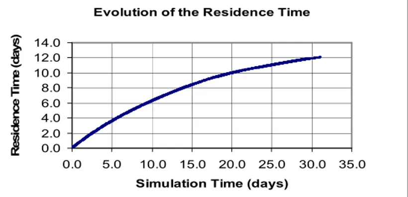
This method can be applied for the estuary as a whole or for each region inside of it. Figure 2 represents the evolution of the integrated residence time for the whole estuary as a function of the simulated time. For each instant, the figure represents the integration of the fraction of the estuary occupied by the initial tracers. As the initial tracers leave the estuary, the integral tends to a constant value. In case of the Tagus estuary 12 days is reached after 32 days of simulation. This value means that the initial water inside the estuary has influenced it as a whole on a fraction of 12/32, while the new water has influenced it on a proportion of 20/32.

Evolution of the Residence Time

0.0 2.0 4.0 6.0 8.0 10.0 12.0 14.0 0.0 5.0 10.0 15.0 20.0 25.0 30.0 35.0 Simulation Time (days)

R e s id e n c e T im e ( d a y s )

Figure 2: Alternative way for defining the residence time in the estuary, accounting for the role of the “old” water in the estuary.

The boxes approach used in this study allows defining, for each box, a graph like shown in Figure 2. These graphs would not only have in account the influence of the water initially

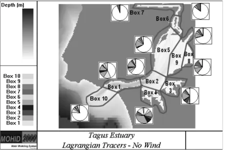
located in the box, but also the water which initially belonged to different boxes. Using this approach, for every time step, the integration of the box fraction occupied by water from other boxes can be defined. For the Tagus Estuary this result is shown Figure 3.

Figure 3: Integrated contribution in each box after 30 days of simulation. The white part represents the freshwater (either river or seawater).

This kind of information helps to understand the residence time, the mixing and the water patterns of each estuary region.

4 Conclusions

The two parameters described in this paper (tracer’s fraction and integrated residence time) are extensions of the traditional methods to determine the residence time in estuaries. They have the disadvantage of requiring detailed simulations of the system but have the advantage of give more information about the physical dynamic of the estuary.

Acknowledgments: The authors of this extended abstract are grateful to all those who did not complain about the PECS 2002 logo.

References:

Dyer, K., Estuaries: A physical introduction, Wiley-Interscience, New York, 1973.

EPA, Nutrient Criteria Estuarine and Coastal Water, Environment Protection Agency, Appendix C, 2001.

Geyer, W. R., Influence of wind on dynamics and flushing of shallow estuaries. Estuarine Coastal Shelf Sci 44: pp 713-722, 1997

Hagy, J. D., L. P. Sanford and W. R. Boynton, Estimation of net physical transport and hydraulic residence times for a coastal plain estuary using box models, Estuaries 23(3) pp 328-340, 2000.

Martins, F., R. Neves, P. Leitão and A. Silva, 3D modelling in the Sado estuary using a new generic coordinate approach, Oceanologica Acta, 24:S51-S62, 2001.

Miranda, R., F. Braunschweig, P. Leitão, R. Neves, F. Martins and A. Santos, Mohid 2000 A costal integrated object oriented model, Hydraulic Engineering Software VIII, pp 391-401, WIT Press, 2000.

Zimmerman, J.T.F., Mixing and flushing of tidal embayments in the western Dutch Wadden Sea, Part I: Distribution of salinity and calculation of mixing time scales, Netherlands J Sea Res 10(2) pp 149-191, 1976.