Then, the pheromone values of all the output connections of the same nodeievaporate.
τijd(t)=
τijd(t)
(1+τk(t)), ∀j∈Ni
whereNiis the set of neighbors of the nodei.
3.6.1.1 ACO for Continuous Optimization Problems ACO algorithms have been extended to deal with continuous optimization problems. The main is-sue in adapting the ACO metaheuristic is to model a continuous nest neighborhood by a discrete structure or change the pheromone model by a continuous one. Indeed, in ACO for combinatorial problems, the pheromone trails are associated with a finite set of values related to the decisions that the ants make. This is not possible in the continuous case. ACO was first adapted for continuous optimization in Ref. [75]. Further attempts to adapt ACO for continuous optimization were reported in many works [224,708,778]. Most of these approaches do not follow the original ACO frame-work [709]. The fundamental idea is the shift from using a discrete probability dis-tribution to using a continuous one (e.g., probability density function [709]).
Initializing the numerous parameters of ACO algorithms is critical. Table 3.6 summarizes the main parameters of a basic ACO algorithm. Some sensitive parame-ters such asαandβcan be adjusted in a dynamic or an adaptive manner to deal with the classical trade-off between intensification and diversification during the search [635]. The optimal values for the parametersαandβare very sensitive to the target problem. The number of ants is not a critical parameter. Its value will mainly depend on the computational capacity of the experiments.
3.6.2 Particle Swarm Optimization
Particle swarm optimization is another stochastic population-based metaheuristic in-spired from swarm intelligence [459]. It mimics the social behavior of natural organ-isms such as bird flocking and fish schooling to find a place with enough food. Indeed, in those swarms, a coordinated behavior using local movements emerges without any central control. Originally, PSO has been successfully designed for continuous opti-mization problems. Its first application to optiopti-mization problems has been proposed in Ref. [457].
TABLE 3.6 Parameters of the ACO Algorithm
Parameter Role Practical Values
α Pheromone influence –
β Heuristic influence –
ρ Evaporation rate [0.01,0.2]
v
Decision space
New position of the particle
Velocity of the particle
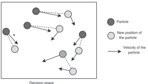
FIGURE 3.33 Particle swarm with their associated positions and velocities. At each iteration,
a particle moves from one position to another in the decision space. PSO uses no gradient information during the search.
In the basic model, a swarm consists of N particles flying around in a D-dimensional search space. Each particle iis a candidate solution to the problem, and is represented by the vectorxiin the decision space. A particle has its own
posi-tion and velocity, which means the flying direcposi-tion and step of the particle (Fig. 3.33). Optimization takes advantage of the cooperation between the particles. The success of some particles will influence the behavior of their peers. Each particle successively adjusts its positionxitoward the global optimum according to the following two
fac-tors: the best position visited by itself (pbesti) denoted aspi=(pi1, pi2, . . . , piD)
and the best position visited by the whole swarm (gbest) (or lbest, the best position for a given subset of the swarm) denoted aspg=(pg1, pg2, . . . , pgD). The vector
(pg−xi) represents the difference between the current position of the particleiand
the best position of its neighborhood.
3.6.2.1 Particles Neighborhood A neighborhood must be defined for each particle. This neighborhood denotes the social influence between the particles. There are many possibilities to define such a neighborhood. Traditionally, two methods are used:
• gbest Method:In the global best method, the neighborhood is defined as the
whole population of particles (Fig. 3.34).
• lbest Method: In the local best method, a given topology is associated with
(b) Local structure: a ring
(a) Complete graph
(c) “Small world graph”
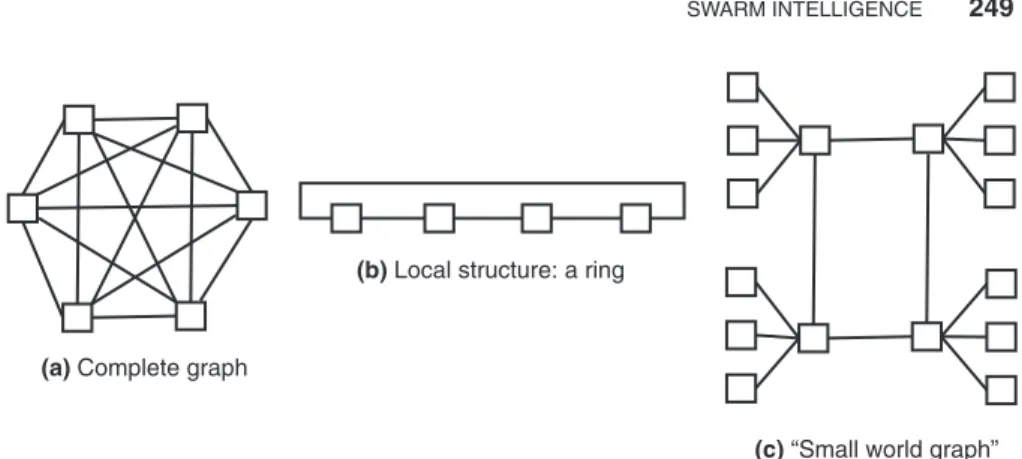
FIGURE 3.34 Neighborhood associated with particles. (a) gbest Method in which the
neigh-borhood is the whole population (complete graph). (b) lbest Method where a noncomplete graph is used to define the neighborhood structure (e.g., a ring in which each particle has two neighbors). (c) Intermediate topology using a small world graph.
graph, ring world graph, and small world graph. This model is similar to social science models based on population members’ mutual imitation, where a sta-bilized configuration will be composed of homogeneous subpopulations. Each subpopulation will define a sociometric region where will emerge a like-minded “culture.” Individuals into the same sociometric region tend to become similar and individuals belonging to different regions tend to be different [40,585].
According to the neighborhood used, aleader(i.e., lbest or gbest) represents the particle that is used to guide the search of a particle toward better regions of the decision space.
A particle is composed of three vectors:
• Thex-vector records the current position (location) of the particle in the search space.
• Thep-vector records the location of the best solution found so far by the particle. • Thev-vector contains a gradient (direction) for which particle will travel in if
undisturbed.
• Two fitness values: The x-fitness records the fitness of the x-vector, and the
p-fitness records the fitness of thep-vector.
A particle swarm may be viewed as a cellular automata where individual cell (particles in PSO) updates are done in parallel; each new cell value depends only on the old value of the cell and its neighborhood, and all cells are updated using the same rules. At each iteration, each particle will apply the following operations:
• Update the velocity:The velocity that defines the amount of change that will
be applied to the particle is defined as
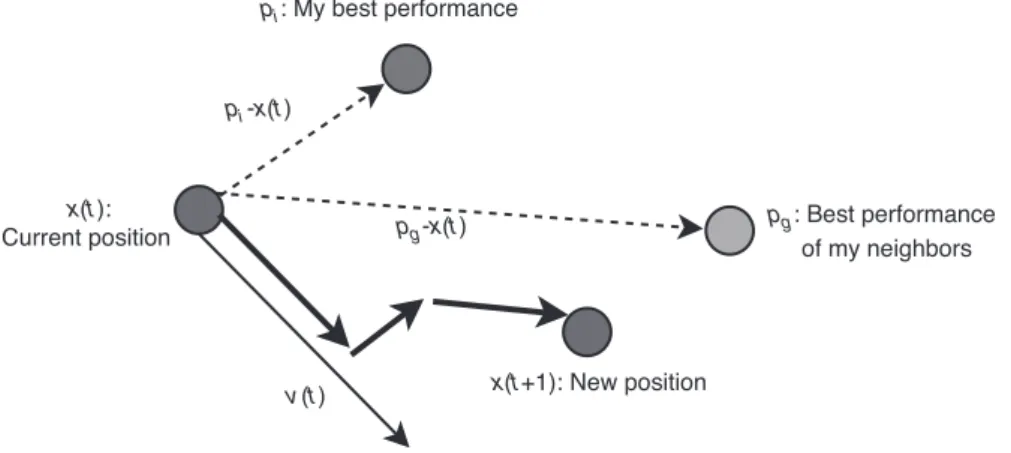
a particle has toward its own success. The parameterC2is the social learning factor that represents the attraction that a particle has toward the success of its neighbors. The velocity defines the direction and the distance the particle should go (see Fig. 3.35). This formula reflects a fundamental aspect of human sociality where the social–psychological tendency of individuals emulates the successes of other individuals. Following the velocity update formula, a particle will cycle around the point defined as the weighted average ofpiandpg:
ρ1pi+ρ2pg
ρ1+ρ2
The elements ofviare limited to a maximal value [−Vmax,+Vmax] such as the system will not explode due to the randomness of the system. If the velocityvi
exceedsVmax(resp.−Vmax), it will be reset toVmax(resp.−Vmax).
In the velocity update procedure, an inertia weightwis generally added to the previous velocity [699]:
vi(t)=w×vi(t−1)+ρ1×(pi−xi(t−1))+ρ2×(pg−xi(t−1))
The inertia weight wwill control the impact of the previous velocity on the current one. For large values of the inertia weight, the impact of the previous velocities will be much higher. Thus, the inertia weight represents a trade-off between global exploration and local exploitation. A large inertia weight en-courages global exploration (i.e., diversify the search in the whole search space) while a smaller inertia weight encourages local exploitation (i.e., intensify the search in the current region).
x(t): Current position
pi: My best performance
pg: Best performance of my neighbors
v(t) x(t+1): New position pg-x(t)
pi-x(t)
• Update the position:Each particle will update its coordinates in the decision space.
xi(t)=xi(t−1)+vi(t)
Then it moves to the new position.
• Update the best found particles:Each particle will update (potentially) the best local solution:
Iff(xi)<pbesti,thenpi =xi
Moreover, the best global solution of the swarm is updated:
Iff(xi)<gbest,thengi =xi
Hence, at each iteration, each particle will change its position according to its own experience and that of neighboring particles.
As for any swarm intelligence concept, agents (particles for PSO) are exchanging information to share experiences about the search carried out. The behavior of the whole system emerges from the interaction of those simple agents. In PSO, the shared information is composed of the best global solution gbest.
Algorithm 3.14 shows the template for the PSO algorithm.
Algorithm 3.14 Template of the particle swarm optimization algorithm.
Random initialization of the whole swarm ;
Repeat
Evaluatef(xi) ;
For allparticlesi
Update velocities:
vi(t)=vi(t−1)+ρ1×(pi−xi(t−1))+ρ2×(pg−xi(t−1)) ; Move to the new position:xi(t)=xi(t−1)+vi(t) ;
If f(xi)< f(pbesti)Thenpbesti=xi;
If f(xi)< f(gbest)Thengbest=xi; Update(xi, vi) ;
EndFor
UntilStopping criteria
Example 3.20 PSO for continuous function optimization. Let us illustrate how
∈
particle will move to its next positionX(t+1). Each particle will compute the next local and global best solutions and the same process is iterated until a given stopping criteria.
3.6.2.2 PSO for Discrete Problems Unlike ACO algorithms, PSO algorithms are applied traditionally to continuous optimization problems. Some adaptations must be made for discrete optimization problems. They differ from continuous models in
• Mapping between particle positions and discrete solutions:Many discrete
representations such as binary encodings [458] and permutations can be used for a particle position. For instance, in the binary mapping, a particle is associated with ann-dimensional binary vector.
• Velocity models:The velocity models may be real valued, stochastic, or based on a list of moves. In stochastic velocity models for binary encodings, the velocity is associated with the probability for each binary dimension to take value 1. In the binary PSO algorithm [458], a sigmoid function
S(vid)=
1 1+exp(−vid)
transforms the velocities valuesviinto the [0,1] interval. Then, a random number
is generated in the same range. If the generated number is less thanS(vid), then
the decision variablexidwill be initialized to 1, otherwise the value 0 is assigned
toxid. The velocity tends to increase when the (p−x) term is positive (pid or
pgd=1) and decreases whenpid orpgd=0. Then, whenvid increases, the
probability thatxid =1 also increases.
Velocity models for discrete optimization problems have been generally in-spired from mutation and crossover operators of EAs.
Example 3.21 Geometric PSO. Geometric PSO (GPSO) is an innovative
Global best
Current position
Best known New
position
FIGURE 3.36 Geometric crossover in the GPSO algorithm.
particlei, three parents take part in the 3PMBCX operator: the current positionxi, the social best positiongi, and the historical best position foundhiof this particle (Fig. 3.36). The weight valuesw1,w2, andw3indicate for each element in the crossover mask the probability of having values from the parentsxi,gi, orhi, respectively. These weight values associated with each parent represent the inertia value of the current position (w1), the social influence of the global/local best position (w2), and the individual influence of the historical best position found (w3). A constriction of the geometric crossover forces
w1,w2, andw3to be nonnegative and add up to 1.
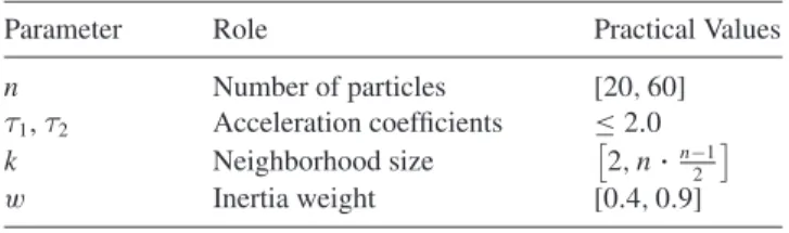
Table 3.7 summarizes the main parameters of a basic PSO algorithm. The number of particlesnhas an inverse relationship with the number of required iterations of the algorithm. Increasing the population size will improve the results but is more time consuming. There is a trade-off between the quality of results and the search time as in any P-metaheuristic. Most of the PSO implementations use an interval of [20,60] for the population size.
The two extremes for the neighborhood sizekare the use of the global population of individuals (k=n(n−1)/2, wherenis the population size) and a local neighbor-hood structure based on the ring topology (k=2). Many intermediate neighborhood structures may be used (e.g., torus, hypercubes). Using large neighborhoods, the con-vergence will be faster but the probability to obtain a premature concon-vergence will be more significant. There is a great impact of the best solution on the whole population
TABLE 3.7 Parameters of the PSO Algorithm
Parameter Role Practical Values
n Number of particles [20,60] τ1,τ2 Acceleration coefficients ≤2.0 k Neighborhood size 2, n
·
n−12
is carried out. This trade-off is similar to the neighborhood size definition in parallel cellular evolutionary algorithms. The optimal answer to this trade-off depends on the landscape structure of the optimization problem.
The relative amount of added elements to the velocitiesρ1andρ2represents the strength of the movement toward the local best and the global best. The two parameters are generated randomly in a given upper limit. Whenρ1andρ1 are near zero, the velocities are adapted with a small amount and the movements of the particles are smooth. This will encourage local nearby exploration. When ρ1 andρ1 are high values, the movements tend to oscillate sharply (see Fig. 3.37). This will tend to more global wide-ranging exploration. Most of the implementations use a value of 2.0 for both parameters [455].
The upper limitVmaxis recommended to be dependent on the range of the problem. This parameter may be discarded if the following formula is used to update the velocities [139]:
vi(t)=χ×(vi(t−1)+ρ1×(pi−xi(t−1))+ρ2×(pg−xi(t−1)))
whereχrepresents the constriction coefficient:
χ= κ
abs
1−ρ2− √
abs(ρ2−4ρ 2
whereκ∈[0,1] (a value of 1.0 has been used),ρ=ρ1+ρ2(should be greater than 4, e.g., limit each ρi to 2.05). Using the constriction coefficient will decrease the
amplitude of the particle’s oscillation.
Landscape
Smooth oscillation Strong oscillation
Objective
Solution 1
1
2 2
3 3
v v
These various parameters may also be initialized in a dynamic or adaptive way to deal with the trade-off between intensification and diversification during the search. Typically, the value of the inertia weightwis initialized to 0.9 to decrease to 0.4. The number of particles can vary during the search. For instance, a particle can be removed when its performance is the worst one [138].
3.7 OTHER POPULATION-BASED METHODS
Other nature-inspired P-metaheuristics such as bee colony and artificial immune sys-tems may be used for complex optimization problem solving.
3.7.1 Bee Colony
The bee colony optimization-based algorithm is a stochastic P-metaheuristic that be-longs to the class of swarm intelligence algorithms. In the last decade, many studies based on various bee colony behaviors have been developed to solve complex com-binatorial or continuous optimization problems [77]. Bee colony optimization-based algorithms are inspired by the behavior of a honeybee colony that exhibits many fea-tures that can be used as models for intelligent and collective behavior. These feafea-tures include nectar exploration, mating during flight, food foraging, waggle dance, and division of labor.
Bee colony-based optimization algorithms are mainly based on three different models: food foraging, nest site search, and marriage in the bee colony. Each model defines a given behavior for a specific task.
3.7.1.1 Bees in Nature Bee is social and flying insect native to Europe, the Middle East, and the whole of Africa and has been introduced by beekeepers to the rest of the world [689,707]. There are more than 20,000 known species that inhabit the flowering regions and live in a social colony after choosing their nest called ahive. There are between 60,000 and 80,000 living elements in a hive. The bee is characterized by the production of a complex substance, the honey, and the construction of its nest using the wax. Bees feed on the nectar as energy source in their life and use the pollen as protein source in the rearing of their broods. The nectar is collected in pollen baskets situated in their legs.
Generally, a bee colony contains one reproductive female calledqueen, a few thousand males known asdrones, and many thousand sterile females that are called theworkers. After mating with several drones, the queen breeds many young bees calledbroods. Let us present the structural and functional differences between these four honeybee elements:
• Queen: In a bee colony, there is a unique queen that is the breeding female