MODELING PORTUGUESE WATER DEMAND WITH QUANTILE
REGRESSION
Maria Leonor Bandeira de Melo Barreiros Cardoso
Project submitted as partial requirement for the conferral of Master in Economics
Supervisor:
Prof. Henrique Monteiro, Prof. Auxiliar, ISCTE Business School, Departamento de Economia
Co-supervisor:
Prof. Maria da Conceição Figueiredo, Prof. Auxiliar, ISCTE Business School, Departamento de Métodos Quantitativos para a Gestão e Economia
Spine
-MO
D
E
L
IN
G
P
O
RT
U
G
U
E
SE
W
A
T
E
R D
E
MA
N
D
W
IT
H
Q
U
A
N
T
IL
E
RE
G
RE
SS
IO
N
Mar
ia Le
ono
r
B
ande
ir
a de
Mel
o
B
ar
rei
ros
Cardos
o
I
A literatura recente sobre a estimação da procura de água indica que a elasticidade-preço da procura de água residencial pode não ser constante ao longo da distribuição do consumo de água. Se assim for, a elasticidade-preço da média da amostra ou da população de consumidores em questão é insuficiente para prever os possíveis impactos de uma mudança de preço.
A aplicação da regressão de quantis para estimar os impactos esperados das variáveis explicativas normalmente aceites na literatura, como é o caso do preço (marginal ou médio), o rendimento ou variáveis relacionadas com o tempo, pretende mostrar que tais impactos são diferentes dependendo dos níveis de consumo de água. Em diferentes percentis da distribuição o efeito dos regressores é diferente.
Os resultados de uma amostra de 383 famílias Portuguesas que são sujeitas a tarifas crescentes por bloco mostram precisamente isso. Especialmente, quando se consideram os efeitos da variável preço, em que as famílias com baixos níveis de consumo de água reagem mais às variações de preço em comparação com as famílias com consumos superiores. Este resultado põe em causa um objetivo comum da estrutura de preços aplicada, onde é esperado que os blocos superiores induzam à poupança de água. Estes resultados mostram que está em falta uma nova reapreciação das estruturas de preços com escalões.
Palavras-Chave: procura residencial de água, regressão por quantis, determinação do preço da água, tarifários com escalões crescentes.
II
Recent research on water demand has pointed out that the price-elasticity of residential water demand may not be constant throughout the consumption distribution. If this is so, knowing the price elasticity of the average of the sample or population of consumers is insufficient to predict the possible impacts of a price change.
The introduction of Quantile Regression to estimate the impacts of explanatory variables, commonly accepted in literature such as price, income or weather variables, aims to show that such impacts differ depending on water consumption levels. At different quantiles of the distribution the regressors effect is different.
The results for a sample of 383 Portuguese households facing increasing-block tariffs show precisely that. Specially, when considering the effects of price, show that low water consumption levels react more to changes in price comparing to high consumption levels. These results contradict one of the common aims of increasing-block tariffs, higher increasing-blocks are expected to induce water savings. The result shows that a rethinking of increasing-block tariffs might be in order.
Keywords: residential water demand, quantile regression, water pricing, increasing-block tariffs.
III
I would like to start to thank to my supervisors Professors Henrique Monteiro and Maria da Conceição Figueiredo, for all the support, help, motivation and availability in all times of necessity. I would like also to express thanks to Professor Catarina Roseta Palma that was a good support when doubts come.
I am grateful for all the support provided from numerous entities. To ISCTE-IUL, for the software and hardware used in this study. To the Sistema Nacional de Informação de Recursos Hídricos (SNIRH) for providing free access to weather data, that otherwise I would not be able to get. To Fundação para a Ciência e Tecnologia (FCT) for the financial support through a research scholarship from the research project “Pricing and behavior responses in the water sector” (reference PTDC/EGE-ECO/114477/2009). At last, but not the least, I recognize and thank all my family and friends for their support during the elaboration of this thesis.
IV
Resumo ... I Abstract ... II Acknowledgements ... III List of Acronyms ... VII Executive Summary ... VIII
I. Introduction ... 1
II. Literature Review ... 3
Portuguese Reality ... 6
III. Empirical Study ... 8
Methodology ... 8
The Model ... 12
Data ... 17
Brief analysis of survey results ... 17
Descriptive statistics ... 20 IV. Results ... 25 Price ... 26 Income ... 28 Average precipitation ... 28 Household size ... 29 Dwelling characteristics ... 29
V. Conclusions and further work ... 31
Bibliography ... 32
V
VI
Table 3: Description of the Water Utilities involved in the survey ... 18
Table 4: Descriptive statistics of the variables ... 21
Table 5: Household distribution among water utilities. ... 21
Table 6: Distribution by household size ... 22
Table 7: Cross table of the monthly net household income and category of schooling of the respondent. ... 23
Table 8: Cross table of monthly net household income and type of dwelling ... 23
Table 9: Cross table of type of dwelling and the main residence of dwelling and if the dwelling has seasonal occupancy. ... 24
Table 10: Quantile regression of log water consumption on marginal price, weather and household characteristics ... 25
Table 11: Quantile regression of log water consumption on average price, weather and household characteristics ... 26
VII
2SLS: Two-stage Least Squares DBT: Decreasing Block Tariffs
EEA: European Environmental Agency
ERSAR: Entidade Reguladora dos Serviços de Água e Resíduos [Regulating Authority on Water and Waste Services]
FCT: Fundação para a Ciência e Tecnologia [Foundation for Cience and Techonology] IBT: Increasing Block Tariffs
ISCTE-IUL: Instituto Universitário de Lisboa [Lisbon University Institute] IV: Instrumental Variables
OECD: Organisation for Economic Co-operation and Development OLS: Ordinary Least Squares
VIII
This thesis aims to estimate residential water demand in Portugal using quantile regression.
An efficient use of water and its preservation is an urgent necessity worldwide. Problems of scarcity and overexploitation in many regions of the world are at the origin of this concern. Therefore it is important to recognize consumer’s behaviors in order to give the right incentives to consumption to reconciling the conflicting goals of water pricing policies like water conservation, efficient use and collecting revenue to cover the costs of providing water services. It is known that when increasing the price of water supplied to consumers, it may have a more significant impact on the utility’s revenues than on water conservation if water demand is inelastic. A common resort for the multiple problem associated is the application of nonlinear prices to water consumption. It is important to know how price-elasticity varies through the distribution in order to define a more precise solution for such a problem.
Portugal applies this nonlinear price structures and as far it is known there are no studies to describe price-elasticity variation through the distribution in the country. This thesis aims to describe that by estimating Portuguese residential water demand using quantile regression. The advantage of using quantile regression is that, as it takes into consideration each quantile of the distribution, it gives a better description of data. The data was collected from a telephone survey to Portuguese households about their water consumption habits and dwelling characteristics, and an estimation considering both marginal and average price was estimated.
Results found out that when considering the effects of price, households with low water consumption levels react more to changes in price comparing to high consumption levels. It is a contradiction to common goals of increasing-block tariffs, induce water savings charging more to higher blocks. Therefore, a reconsideration of increasing-block tariffs structure is needed to keep pursuing such objectives.
1
I.
Introduction
The efficient use of such a vital natural resource as water is a growing concern throughout the world. Recent reports by the European Environment Agency (EEA) (EEA, 2009) and (EEA, 2012) show an increasing concern with water scarcity and overexploitation in many regions of the world. This is not only due to increasing consumption but also to the impacts of climate change in the availability of water. (EEA, 2007) analyses the impacts of climate change on European water resources and the adaptation measures involved. Namely for Portugal a change in precipitation patterns is predicted with concentration in the winter months, thus reducing surface water flows in the summer with impacts on diminished water quality, especially in the South. This is a growing concern especially regarding the quality of water stored in reservoirs (OECD, 2011 a).
(EEA, 2009) and (EEA, 2012) explicitly recognize that water pricing and other economic instruments are essential for sustainable water management not only to safeguard the quantity and quality of water available for use by humans and for environmental purposes, but also to ensure the financial sustainability of the water utilities providing water supply and sanitation service. This is not a European feature as other international institutions have been recognizing the key role of providing the right economic incentives to change consumer behavior (OECD, 2011 b).
Reconciling the conflicting goals of water pricing policies like water conservation, efficient use and collecting revenue to cover the costs of providing water services requires the knowledge of the consumers’ response to prices (Griffin, 2006). Increasing the price of water supplied to consumers may have a more significant impact on the utility’s revenues than on water conservation if water demand is inelastic. Recent research has pointed out that price-elasticity of residential water demand may not be constant throughout the consumption distribution with some consumers adapting more to price hikes, while others may prefer to pay the price of maintaining their level of consumption (Monteiro and Roseta-Palma, 2011), (Mylopoulos, et al., 2004) and (Renwick and Archibald, 1998).
2
Pricing policies for water supply often resort to nonlinear prices, namely using two-part tariffs, where the variable component may include several blocks usually increasing in price. (OECD, 2010) reports an emerging trend in some OECD countries in the use of this type of tariff structure. Although this is only a second-best approach in this multiple-goal price-setting context, it should nonetheless be well-informed about the impacts of the tariff structure and price levels on the water utility’s revenues and on the amount of water consumed. The knowledge of the price-elasticity of water demand for the average of the sample or population of consumers is insufficient to predict the possible impacts of a proposed price change if consumers’ response to price differs across the distribution of consumption levels.
We use quantile regression to get estimates of the impacts that different relevant explanatory variables (including price) may have on water consumption for different consumption quantiles in order to get a more accurate picture of the full impact of price changes. The thesis is structured as follows. Section 2 presents a literature review on water demand and quantile regression as well as an overview of the Portuguese water sector. Section 3 describes the methodology applied; presents data source and describe the sample. Section 4 shows the results at different quantiles of the distribution, and finally Section 5 offers concluding remarks on results.
3
II.
Literature Review
The stream of residential water demand research has been affluent since the 1950’s and it continues to add to the literature nowadays, stimulated by the increasing need to encourage an efficient use of the resource. (Arbués, et al., 2003) and (Worthington and Hoffman, 2008) are the most recent surveys on this literature. (Dalhuisen, et al., 2003) is also an important reference that enables us to learn the characteristics and focus of this strand of research.
The quantity demanded of water by households is a function of several variables, most prominent among them, its price. According to consumer theory, water consumption is expected to be inversely related to water price. Empirical studies have shown the percentage change in quantity demanded as a response to a price change to be less than the percentage change in price, evidence of an inelastic price-elasticity of demand. A distinctive feature of water prices is that they are often nonlinear and, if that is the case, the researcher estimating water demand must take that into account to avoid the serious problem of biased estimates because of endogenous regressors, given that with nonlinear prices the marginal and the average price paid by the consumer depends on the amount of water consumed (Monteiro, 2009). In general, consumers face a fixed fee and pay an additional price per unit of water consumed, where this variable part of the tariff structure is often a block tariff. Therefore, nonlinear tariffs arise not only due to the use of two-part tariffs but also due to the use of blocks in the variable component. With block tariffs, water price structures are discontinuous. Different prices are set for several levels of consumption. Block tariffs can be increasing (IBT) if the price increases with consumption or decreasing (DBT) if the price decreases when the volume of consumption is higher. The use of IBT aims to promote water conservation (charging higher prices for the upper blocks) and accessibility of the service (through lower price for the first blocks people with less resources can have access). Facing such a complex tariff scheme makes it difficult for consumers to have full information about the price structure, making it hard to analyze changes in the intramarginal rates, for example.
4
To estimate residential water demand it is standard to use other independent variables such as household income, weather variables (precipitation, temperature), household size and composition, educational campaigns among others. Income can be introduced as per household or per capita or, if unavailable, be replaced by wealth proxy variables such as the assessed value of property, as in (Worthington and Hoffman, 2008).
Usually income appears as inelastic and with small magnitude, sometimes it is argued that it happens due to the fact that water bill represents a small proportion of households income (Agthe and Billings, 1987), (Saleth and Dinar, 2000), (Gaudin, et al., 2001), (Garcia and Reynaud, 2003).
Water consumption is seasonal, namely for outdoor uses, people tend to consume more in the summer than in the winter due to the high temperatures felt at that time of the year and the lower precipitation levels, therefore the inclusion of weather variables is of an extreme importance. (Worthington and Hoffman, 2008), for example found that “summer price elasticities are lower than winter price elasticities”. (Foster and Beattie, 1979, 1981), (Espey and Shaw, 1997), (Dalhuisen, et al., 2003) found evidence that the incorporation of precipitation as an explanatory variable generates less price-elastic estimates of water demand. (Griffin and Chang, 1990), (Stevens, et al., 1992), (Agthe and Billings, 1987) and (Hoffman, et al., 2006) used temperature, as average monthly temperature, number of sunny days or number of days with temperature exceed 58ºF. (Billings, 1982), (Agthe, et al., 1986), (Nieswiadomy and Molina, 1988) and (Hewitt and Hanemann, 1995) used in their studies evapotranspiration, which accounts for the evaporation and plant transpiration on land surface to atmosphere.
Household size and composition can influence water consumption. A larger household will consume more and the presence of children in the household will also increase consumption. As shown by (Nauges and Thomas, 2000), children don’t take into consideration the amount of water they are spending, take longer baths and do a lot of water-intensive outdoor activities which implies, that younger populations tend to consume more than older ones. (Martínez-Espineira, 2003) includes the proportion of population over 64 and those less than 19 years old to cover the differences in household composition, and reaches the same result. (Griffin and Chang, 1990), and (Gaudin, et al., 2001) have also shown that population origin also affects water consumption in a way that people with a latin cultural background tend to consume
5
more. Other non-price consumption controls, as water conservation and educational campaigns or restrictions on water use have been used to explain differences in water demand. However as shown in (Syme, et al., 2000), this type of measures are difficult to evaluate in terms of its efficacy, mostly due to multicollinearity among variables, problems of interpretations or unmeasured variables. For example if the government imposes a program on water saving to be teach in school it is difficult to evaluate how much children from the course, are saving compared to those that have not the course. When authors try to value such a program tend to face those difficulties as seen in as (Renwick and Green, 2000), (Gaudin, 2006), (Martínez-Espineira, 2007). More variables have been applied to estimate residential water demand but they are not consensual in literature, representing only some questions about specific researches, like home ownership (Nieswiadomy, 1992), pool ownership (Dandy, et al., 1997) or water saving devices (Renwick and Archibald, 1998) and (Yoo, 2007).
Most early studies compile US data (Gaudin, et al., 2001), (Timmins, 2002), however nowadays it is really common to see European data, for example from Spain and France (Nauges and Thomas, 2000), (Martínez-Espineira, 2002) and (Nauges and Thomas, 2003) as well as data from development countries. There are only two studies using Portuguese data (Martins and Fortunato, 2007), (Monteiro and Roseta-Palma, 2011). However there is no previous research covering micro level data. It is difficult to perform micro level data studies, due to the need of a great volume of information and the low access to good sample micro data (Worthington and Hoffman, 2008). That is a possible explanation for the small number of micro data studies compared to aggregate data studies despite the fact that a residential household demand approach is preferred to an aggregate/municipal approach (Arbués, et al., 2003).
A wide range of data type is applied. Just to name a few examples, (Agthe and Billings, 1980), (Chicoine and Ramamurthy, 1986), (Hewitt and Hanemann, 1995), (Dandy, et al., 1997), (Gaudin, et al., 2001), (Martínez-Espineira, 2003) used panel data, while (Stevens, et al., 1992), (Rietveldt, et al., 2000), (Hadjispirou, et al., 2002) used cross-sectional data. Some studies have also used time-series (Billings and Agthe, 1998) or pooled data.
Early studies on residential water demand estimation resorted to mostly to ordinary least squares (OLS) techniques as (Hewitt and Hanemann, 1995), (Higgs and Worthington,
6
2001) or (Hoffman, et al., 2006) (to see more studies on this see the list on (Monteiro, 2009), however it is possible to find studies using two-stage and three-stage least squares (Nieswiadomy and Molina., 1991), or IV methods, to deal with the problem of endogeneity that appears from water price structure, where quantity consumed determines the price and vice versa, (Agthe and Billings, 1980), (Hewitt and Hanemann, 1995), (Barkatullah, 1996), (Renwick and Archibald, 1998), (Higgs and Worthington, 2001), (Nauges and Berg, 2008),and (Kenney, et al., 2008). Moreover it is also possible to find other methods as maximum likelihood estimation in (Olmstead, 2009), panel data estimators in (Bell and Griffin, 2008) and (Monteiro and Roseta-Palma, 2011), and time-series techniques in (Azomahou, 2008) and (Martínez-Espineira and Nauges, 2004).
A large diversity of econometric methods have been applied in this literature, however as far as we known, there are no published researches on residential water demand applying quantile regression to water demand estimation. (Koenker and Bassett, 1978) introduced the Quantile Regression (QR) model, a model where each conditional quantile has a linear form, representing the relationship between the dependent variable and the regressors at different points in the distribution. This method benefits from being more robust to outliers than least-squares regression, from being more consistent under weaker stochastic assumptions than least-squares and providing a better characterization of data (Cameron and Triverdi, 2005). Once it is possible to characterize the entire conditional distribution. The advantage of introducing this econometric method into residential water demand estimation is the possibility to perform a better characterization of how water consumption depends on the variables described such as income, weather and price. With a full representation of high and low water consumers, water utilities and policy makers could better design water tariffs and water policies to achieve the several goals they need to meet (efficiency, cost-recovery and water conservation among others).
Portuguese Reality
The Portuguese water sector is responsible for the activities of providing water to rural or urban populations and to the urban economic activities, such as industry and
7
commerce, as well as the drainage and treatment of urban wastewater. Utilities should provide a quality service at fair price, following the principles of general access, continuity and quality of the service, efficiency and equity of the prices (Portuguese entity for regulation of water and wastewater (ERSAR) website). The services are provided by nearly five hundred management utilities all around the country (including islands), either state-owned, municipally-owned companies, municipal services or private concessions (ERSAR, 2012). It is a very dynamic and complex sector due not only to the number of utilities but also to the different size, capacity and available resources of each utility. Financially the sector is highly dependent of European Community funds as the European Regional Development Fund and Cohesion Fund to develop new necessary distribution infrastructures. The sector is regulated by ERSAR which verifies through all utilities the uniformization of procedures and ensures that the interests of consumers are satisfied (ERSAR, 2011 and 2012).
The sector is considered as a natural monopoly; the average cost is decreasing over the relevant output range, called economies of scale. When economies of scale exist it is difficult for companies to provide the same services. Therefore in the presence of a large cost advantage the best thing is to having all industry’s output produced by a singel firm. Prices are set individually by each utility and follow a mixture of fixed and variable components normally applied in the form of IBT.
8
III.
Empirical Study
Methodology
This section discusses the econometric method associated to the estimation of Portuguese water demand.
Quantile Regression analyses the entire conditional distribution of the dependent variable, through the distribution’s quantiles. One can say that it is a method that models conditional quantiles for any quantile value, in that way it computes several regressions for the different quantiles between 0 and 1. It gives an idea of the impact of the independent variables on the entire distribution. This is an advantage compared to OLS that describes how the dependent variable’s mean varies conditional on numerous regressors, in other words it estimates the conditional mean of the dependent variable. In OLS there is no assumption made about the distribution of the errors, the models are estimated consistently, if it is verified that the model has presence of heteroskedasticity or auto correlation it can be adjusted for inference matters.
QR intends to go further and give a more complete picture of the relationship of dependent and independent variables.
The first seminar paper on quantile regression was written by (Koenker and Bassett, 1978), where the aim of the model and its usefulness is explained. The model is described as following the (Buchinsky, 1998):
( | ) ( ) (3.1) where and are Kx1 vectors. And ( | ) denotes the conditional quantile of given . Also, let ( | ) be the density of given , it is unspecified once the distribution of ( ).
In the general case, the sample quantile, where ( ). The QR estimator minimizes the objective function:
( ) ∑ | | ∑ ( )| |
9
It estimates the vector of coefficients for each value of . When , we have the least absolute-deviations estimator that minimizes ∑ | | which is also called
the median estimator. It can be rewritten as
∑ ( ) (3.3) Where can assume the value of if or if , it is a check function. As so it can be rewritten as
[∑ { } | | ∑ { }( )| |] (3.4) The solution of the minimizing problem does not have an explicit solution since the objective function (3.4) is linear and continuous. Therefore, to obtain the solution there is the need of call on some iterative linear programming techniques, see (Koenker and Basset, 1978) and (Koenker, 2005) to analyze a more detailed solution.
Using QR provides some advantages, as discussed in (Buchinsky, 1998) and (Koenker and Hallock, 2001). First, as it is possible to study the impact of a single covariate through the full distribution of the dependent variable, it gives a better representation of data, and no constraints are enforced on the error term. Second, it is more robust to outliers than OLS regression and is more consistent under weaker stochastic assumption. Finally, it is invariant to any monotone transformation of the dependent variable, fact that is only true for OLS if the transformation is linear. Consequently, it is very useful to apply to such a heterogeneous data as household level data, because one can analyze how parameters vary across different quantiles of the distribution. It is very good in particular, when compared to OLS that has constant parameters over the distribution, meaning that everyone on average has the same impact, something that may not be representative of the reality. However, if it really does not change much over the distribution QR will have the same parameters, if the contrary happens it show us the real picture of the distribution.
When estimating any model one should take into consideration the assumptions made in order to conclude with some degree of confidence. An important assumption is the exogeneity assumption, where the error has an expected value of zero given any
10
values of the independent variables: ( | ) . In regular OLS estimation, when the exogeneity hypothesis is not satisfied, at least one of the regressors is correlated to the error term, meaning it is endogenous. To correct for this and achieve consistent estimators, the two stages least squares (2SLS) can be used. As described in (Wooldridge, 2009) and following its notation:
(3.5) Where the independent variable ( ) is endogenous as it is correlated with , meaning that ( ) . Usually, a solution for this problem of lack of consistency in the estimator can be implemented if a new variable ( ), called instrumental variable (IV), that is not correlated with the error term ( ) but is correlated, either positively or negatively, with , the endogenous explanatory variable.
When discussing the application of multiple IV variables it is possible to find a linear combination that is also uncorrelated with .
(3.6) where ( ) , ( ) , ( ) and ( ) . IV variables should not be perfectly correlated with , at least one of or must be significantly different from zero for the model to be identified.
First, (3.6) is computed to obtain the fitted values:
̂ ̂ ̂ ̂ ̂ (3.7) It is verified that variables and jointly significant at a reasonably small significance level, it means that the introduced variables are good and can be used as IV for .
In the second stage an OLS regression is performed, where is used in place of : (3.8) At this point the composition error ( ) has zero mean and is uncorrelated with and . Where the IV estimates are identical to the OLS estimates from the regression of
1
.
The use of IV in QR is a rather new subject and has lack of software packages and development. It was introduced with a model of quantile treatment effects in the presence of discrete endogenous regressors by (Chernozhukov and Umantsev, 2001).
1
11
They have defined several conditions that concern spatial probabilities in order to get consistency and a couple of conditions for identification with some functional form assumptions. The topic was also analyzed by (Abadie, et al., 2002) and (Arias, et al., 2001). The former has used the estimation in two-step methods, as in 2SLS which is the one applied in this thesis.
The method consists in, firstly, regressing the endogenous variable on the exogenous variables built-in in the model (including the instrument or the instruments if there are more than one IV variables) with least squares, and afterwards in a second step it is estimated a quantile regression model of the first equation defined with the predicted values of the endogenous variable included. The entire system is estimated with bootstrap techniques.
It is a common approach in QR to estimate the standard errors with bootstrap (“an approximation of the distribution of a statistic by a Monte Carlo simulation, with sampling done from the empirical distribution or the fitted distribution of the observed data” (Cameron and Tiverdi, 2005), as it is estimated in (Koenker, 2005) an in (Cameron and Triverdi, 2005). Bootstrap was presented by (Efron, 1979) which clarifies that is no less than constantly resampling of the same size from the initial sample with some replacements, as a purpose of reducing the intervals of confidence. It is important to take into consideration that there are no asymptotic results for IV in QR. Future research in the field could check the convergence of bootstrap estimation to the parameter’s real value. The model presented below was estimated computationally using 1000 replications.
There was the need for test some equality of quantiles, to make sure that the coefficient impact is not the same throughout the quantiles. This can be tested with a simple F-test where the null hypothesis is as following:
( ) ( ) (3.9) and the test statistics is:
( ) ( )
12
Where the formula of the asymptotic variance, ̂( ), is described in Koenker (2005) page 75.The usefulness of the test relies on the importance of knowing if the coefficients really differ across quantiles. This is something impossible to test in OLS.
The Model
It has been proven that variables such as price, weather variables such as temperature and precipitation or household characteristics influence water demand. Our main goal is not to find new covariates that influence water consumption, therefore we follow the literature in the choice of our regressors.
Price is a crucial variable when water demand is estimated. Usually authors follow (Shin, 1985), for example (Monteiro, 2009) and (Nieswiadomy and Molina, 1991), to test whether consumers tend to respond to average price or marginal price. However, as far as it is known there is no application of these tests to QR. Therefore, we cannot test whether people respond to variations in average price or in marginal price. Consequently, the demand estimation was developed with two models, one taking into account the marginal price and the other with the average price. It was possible to gather household water consumption data during one year, which was combined with survey data. The models to be estimate are:
Model A: (3.12) Model B: (3.13) In Table 1 it is described the variables included in the model.
13
Table 1: Description of model variables
Variable Description Source
Logarithm of the monthly average water consumption of the household July 2011-June 2012 in m3
Data provided by water
utilities Logarithm of the marginal price in € of for the average
monthly consumption (reference month: June 2012; includes all components indexed to water consumption: water supply, sanitation, solid waste when applicable, water resources tax and value-added tax)
Own calculations
Logarithm of the average price in € for the average monthly consumption (reference month: June 2012 ; includes all components indexed to water consumption: water supply, sanitation, solid waste when applicable, water resources tax and value-added tax)
Own calculations
Logarithm of the long-term average monthly precipitation in mm from 1980 to 2012
SNIRH
Monthly after-tax household income (=1 if the net household income is greater than 501€, =0 otherwise)
Survey data
Household size Survey data
Type of dwelling (=1 if the dwelling is a detached or semidetached house, =0 otherwise)
Survey data
Number of taps in the dwelling Survey data
Existence of a bathtub (=1 if there is a bathtub in the dwelling, =0 otherwise)
Survey data
Existence of a washing machine (=1 if there is a washing machine in the dwelling, =0 otherwise)
Survey data
Existence of a dishwasher ( =1 if there is a dishwasher in the dwelling, =0 otherwise)
Survey data
Existence of a shower (=1 if there is a shower in the dwelling, =0 otherwise)
Survey data
Seasonal dwelling (=1 if the dwelling is has seasonal occupancy, =0 otherwise)
14
The selection of a log-log model was due to the sake of simplicity. Having this type of model, where quantities and price are related in logs, has the advantage that coefficients can be interpreted as elasticities.
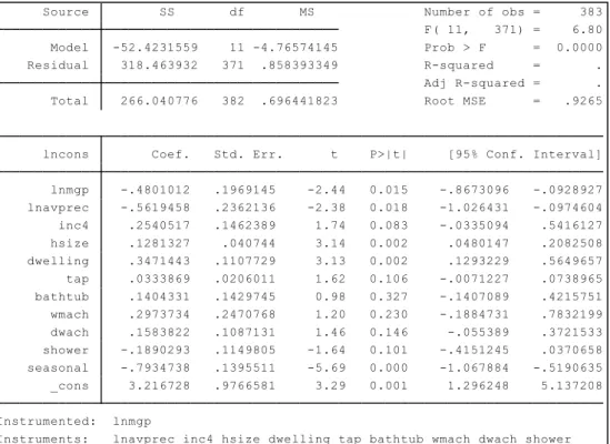
There was a special focus on the price variable. Marginal and average prices were computed from the tariff structure with the help of Microsoft Excel for the average monthly household water consumption provided by the water utilities for each observation. The marginal price is interpreted as the increment in price for an increase of one cubic meter consumed. And the average price was calculated as the average price paid for each cubic meter consumed during the year of analysis. As mentioned before Portugal applies IBT to its water tariffs. Hence, not only does the quantity demanded depend on the price but also the marginal and the average prices depend on how much water the household consume during the billing period. This means for example that a household’s water savings will be reflected not only in a lower water bill but also in a smaller price for each m3 of water. As a result, price can be a source of endogeneity, a problem which can lead to biased coefficients, an obvious undesirable feature in a estimation. A call for instrumental variables estimation is in order to correct such situation. The IV variables selected to this demand estimation follow a similar procedure as in (Deller, et al., 1986), (Reynaud, et al., 2005), (Olmstead, 2009), (Ruijs, et al., 2008) and (Monteiro, 2009). We used information from the tariff schedule, as it is possible to see from Table 2 it is used the marginal price of water supply and sewage of 5 and 25 cubic meters and the other variables included in the model. 5 and 25 cubic meters represent the first and last block of price structure, respectively.
Table 2: Description of variables used as instruments of avp and mgp
Variables Description
m3_5_12 Marginal price of water supply and sewage for a consumption of 5 cubic meters (reference month: June 2012; includes all components indexed to water consumption: water supply, sanitation, solid waste when applicable, water resources tax and value-added tax)
m3_25_12 Marginal price of water supply and sewage for a consumption of 25 cubic meters (reference month: June 2012; includes all components indexed to water consumption: water supply, sanitation, solid waste when applicable, water resources tax and value-added tax)
15
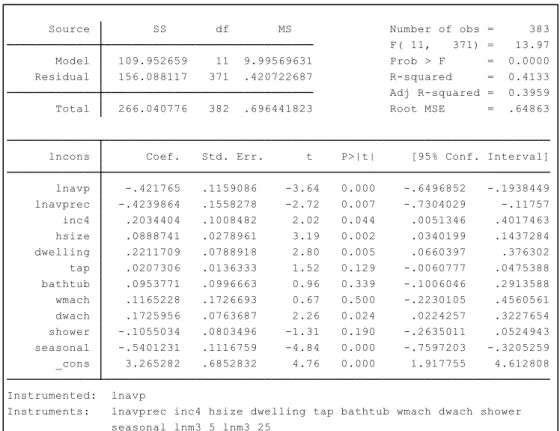
The IV equations are described in (3.14) and (3.15) where heteroskedasticity is taken in consideration with the calculation of robust standard errors:
(3.14) (3.15) seasonal lnm3_5 lnm3_25
Instruments: lnavprec inc4 hsize dwelling tap bathtub wmach dwach shower Instrumented: lnmgp _cons 3.216728 .9766581 3.29 0.001 1.296248 5.137208 seasonal -.7934738 .1395511 -5.69 0.000 -1.067884 -.5190635 shower -.1890293 .1149805 -1.64 0.101 -.4151245 .0370658 dwach .1583822 .1087131 1.46 0.146 -.055389 .3721533 wmach .2973734 .2470768 1.20 0.230 -.1884731 .7832199 bathtub .1404331 .1429745 0.98 0.327 -.1407089 .4215751 tap .0333869 .0206011 1.62 0.106 -.0071227 .0738965 dwelling .3471443 .1107729 3.13 0.002 .1293229 .5649657 hsize .1281327 .040744 3.14 0.002 .0480147 .2082508 inc4 .2540517 .1462389 1.74 0.083 -.0335094 .5416127 lnavprec -.5619458 .2362136 -2.38 0.018 -1.026431 -.0974604 lnmgp -.4801012 .1969145 -2.44 0.015 -.8673096 -.0928927 lncons Coef. Std. Err. t P>|t| [95% Conf. Interval] Total 266.040776 382 .696441823 Root MSE = .9265 Adj R-squared = . Residual 318.463932 371 .858393349 R-squared = . Model -52.4231559 11 -4.76574145 Prob > F = 0.0000 F( 11, 371) = 6.80 Source SS df MS Number of obs = 383
Figure 1: Instrumental Variable (2SLS) regression for lnmgp
Fonte: Stata
16
seasonal lnm3_5 lnm3_25
Instruments: lnavprec inc4 hsize dwelling tap bathtub wmach dwach shower Instrumented: lnavp _cons 3.265282 .6852832 4.76 0.000 1.917755 4.612808 seasonal -.5401231 .1116759 -4.84 0.000 -.7597203 -.3205259 shower -.1055034 .0803496 -1.31 0.190 -.2635011 .0524943 dwach .1725956 .0763687 2.26 0.024 .0224257 .3227654 wmach .1165228 .1726693 0.67 0.500 -.2230105 .4560561 bathtub .0953771 .0996663 0.96 0.339 -.1006046 .2913588 tap .0207306 .0136333 1.52 0.129 -.0060777 .0475388 dwelling .2211709 .0788918 2.80 0.005 .0660397 .376302 hsize .0888741 .0278961 3.19 0.002 .0340199 .1437284 inc4 .2034404 .1008482 2.02 0.044 .0051346 .4017463 lnavprec -.4239864 .1558278 -2.72 0.007 -.7304029 -.11757 lnavp -.421765 .1159086 -3.64 0.000 -.6496852 -.1938449 lncons Coef. Std. Err. t P>|t| [95% Conf. Interval] Total 266.040776 382 .696441823 Root MSE = .64863 Adj R-squared = 0.3959 Residual 156.088117 371 .420722687 R-squared = 0.4133 Model 109.952659 11 9.99569631 Prob > F = 0.0000 F( 11, 371) = 13.97 Source SS df MS Number of obs = 383
To test if the instruments applied were good enough an Anderson test was performed. If the null hypotheses of underidentification is rejected, which it is in both models (Appendix A and B), it means that the used instruments are relevant. When looking at the Sargan test both models are not rejected which implies the validity of the instruments. Afterwards an endogeneity test was performed to both models and it is corrected after using the proposed instruments. There was no need to worry more about biasness of estimators in general, once endogeneity is already accounted for.
It is important to have a meteorological variable in the model. However, there are few freely available data on precipitation and temperature. After some digging it was found the National Water Resources Information System (SNIRH) website2, which has available data for Portuguese temperature and precipitation since 1980. However, the maintenance of automatic monitoring stations has been suspended since mid-March 2010 due to the economic problems Portugal is facing. Therefore, there is a high
2
http:/snirh.pt
17
probability of gaps in the used data. Given this constraint, the precipitation data is not entirely reliable. We selected the average monthly accumulated precipitation. It is accumulated in the sense that the average is weighted on all monthly precipitation observations (since 1980 until 2012). This type of data was already applied by (Gaudin, 2005) and (Gaudin, 2006).
Income is a dummy variable that assumes the value 1 for all households that have a monthly net income larger than or equal to 501€. It was computed form the income question of the survey described below. To avoid a large proportion of people refusing to answer the amount of money earned in a month, the question was categorical. Households were only asked to name which category was representative of their situation. Even in this way it was one of the questions with a larger non-response rate. From the question’s results, income was rearranged in two groups, one where households earn up to 500€ and another where households make at least 501€ each month. The income variable was used in this way in both models.
Data
Brief analysis of survey results
The data was collect from a survey done in the summer of 2012 to 2.440 households from 13 Portuguese water utilities (see Table 3) that agreed to participate in the research. These utilities are not well distributed among country regions3, and therefore it lacks of representativeness of Portuguese’s population distribution. Therefore the surveyed households are not illustrative of Portuguese water consumption.
18
Table 3: Description of the Water Utilities involved in the survey
Water Utilities
Águas do Sado (AS)
Câmara Municipal de Lagos (CML)
Câmara Municipal de Montemor-o-Velho (CMMV) Câmara Municipal de Sines (CMS)
Câmara Municipal de Vila de Rei (CMVR) Câmara Municipal de Vouzela (CMV)
Empresa Municipal de Águas e Resíduos de Portimão (EMARP) Empresa Municipal de Água e Saneamento de Beja (EMAS) Serviços Municipalizados Alcobaça (SMA)
Serviços Municipalizados de Água e Saneamento das Caldas da Rainha (SMASCR) Serviços Municipalizados de Saneamento Básico de Viana do Castelo (SMSBVC) Serviços Municipalizados de Água e Saneamento da Guarda (SMASG)
Serviços Municipalizados de Água e Saneamento de Sintra (SMASS)
The survey’s purpose was to get household level data for more adequate water demand estimation, where respondents were asked questions related to their household and dwelling characteristics, as income, number of household members, employment status, car ownership, pool ownership, type of dwelling, number of taps, number of bathtubs and showers, as well as water consumption behavior, as bath/shower or gardening habits. Questions about behavioral characteristics and environmental concerns were asked through open questions. Survey questions are available upon request. Information about the specific household consumption was provided a posteriori by each water utility. Consumption information covered by water utilities was the amount of water consumed per month, in m³, by each household during the billing period, the corresponding readings of each billing period made to those households, bill information and tariff information corresponding to the period in analysis.
The survey was conducted by telephone between June and August 2012, where the "questioner" registered all the answers into data collection software (Qualtrics). The survey questions were related to the 12 months immediately before to the survey, from
19
July 2011 to June 2012. The water utilities were chosen based on willingness to participate and 13 agreed to do it. Since participant water utilities were not representative of population distribution in the country, there was no effort to ensure the representativeness of the sample. However there was a concern to randomly choose the respondents within each utility. The survey was performed within the framework of the research project "Price and behavioral responses in the water sector", reference PTDC/EGE-ECO/114477/2009, funded by Foundation for Science and Technology (FCT).
The participating water utilities provide water services to 422.558 consumers. Although, the survey was only conducted to 2.440 households it was only possible to obtain water consumption data from 2.386 households.
Half of the completed surveys were responded by females, and half of them have completed at least one year of secondary school, equivalent to 12 years of schooling more or less. The sample average household size is 2,7 persons and 51% have more than 3 members. 53% of the surveyed persons were working, however, only half of the households have monthly net income over 1.000€.
Approximately 80% of the dwellings are owned by the families living there, and 51% are semi-detached or detached houses. Only 3% of them have a pool and 37% have a garden or a backyard. 64% of the dwellings are equipped with shower-bath facilities and on average there are 6,3 taps per dwelling. From the surveyed dwellings, 95% have a washing machine and only 63% have a dishwasher.
Although only 14% of the whole sample has an alternative to the publicly supplied water, there is one water utility where 56% of the households have other alternatives of water supply. 42% of surveyed household’s members tend to drink tap water instead of bottled water, however in some water utility areas only 18% of them prefer to drink tap water when compared to bottled water.
When analyzing the water bill information, 69% of the surveyed persons claimed to be always aware of the billing information but only 54% of them know the details of the bill. When asked about the water tariff structure 74% of the household do not answer, and 79% of them say that it includes no more than 3 blocks. Actually, for the water utilities considered in the survey the number varies between 4 and 6 blocks. Only 3% of
20
the answers were correct, moreover only 8% of the households knew the price per cubic meter of the water they are consuming. We conclude that consumers tend to believe they are aware of their water tariff, but that is not true. Actually, they don’t know the average price and have a tendency to underestimate it. The amount of water consumed is usually overestimated among consumers. However, they tend to know the total amount of water bill.
When analyzing the billing period of water utilities, we found that all utilities have the same billing period, monthly, but not all consumed meters were read every month. It is usual to intercalate meter readings with estimates done by the water utility based on past consumption. Data for consumption was provided for the period from July 2011 to June 2012. We opted to use only actual meter readings and exclude estimates, leaving us with 505 households to study. Moreover sometimes household left some survey questions unanswered so when selecting variables to use in the model, additional observations were lost, leaving data for 383 households.
Descriptive statistics
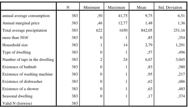
The following section contains information about the variables included in the water estimation. The common descriptive statistics are included in Table 4.
21
Table 4: Descriptive statistics of the variables
N Minimum Maximum Mean Std. Deviation
annual average consumption 383 ,50 41,75 9,75 6,51
Annual marginal price 383 ,46 12,77 1,48 1,36
Total average precipitation 383 622 1650 842,05 251,16
more than 501€ 383 0 1 ,85 ,354
Household size 383 1 14 2,79 1,291
Type of dwelling 383 0 1 ,57 ,496
Number of taps in the dwelling 383 2 24 6,67 3,045
Existence of bathtub 383 0 1 ,83 ,380
Existence of washing machine 383 0 1 ,95 ,217
Existence of dishwasher 383 0 1 ,62 ,486
Existence of a shower 383 0 1 ,63 ,483
Seasonal dwelling 383 0 1 ,17 ,374
Valid N (listwise) 383
In Table 5 the household distribution among the supportive water utilities is not representative sample of Portuguese population. It is possible to see that the North region has 27 households, Center 137, Lisbon has only 11 households, Alentejo 146 households and the last one Algarve has 62 interviewed households.
Table 5: Household distribution among water utilities.
Frequency Percent Águas do Sado 11 2,9 CM Lagos 45 11,7 CM Montemor-o-Velho 87 22,7 CM Sines 146 38,1 CM Vila de Rei 44 11,5 CM Vouzela 1 ,3 EMARP 17 4,4 SMAG 1 ,3
SMAS Caldas da Rainha 5 1,3
SMSBVC 26 6,8
Total 383 100,0
22
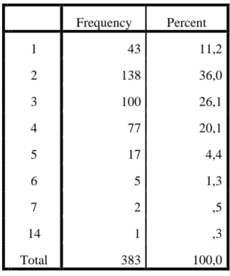
Table 6 shows the distribution of households by household size. We can see that 36% of households have 2 members and 26.1% have 3 members.
Table 6: Distribution by household size
Frequency Percent 1 43 11,2 2 138 36,0 3 100 26,1 4 77 20,1 5 17 4,4 6 5 1,3 7 2 ,5 14 1 ,3 Total 383 100,0
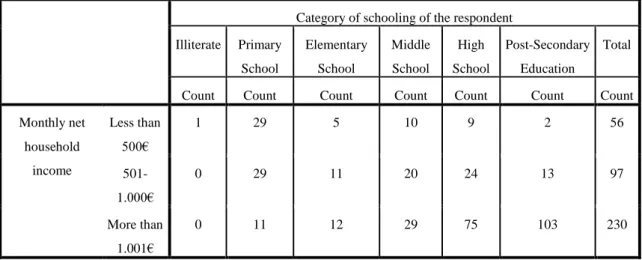
In order to describe the data some cross tables are presented with relevant information about the consumers. From Table 7 one can see that most households live with more than net 1.000€ per month. Households with lower levels of net monthly income have less years of schooling. Likewise households with more net income have more years of schooling. In that way, for households with a net income of at most 500€ per month the respondent has, most of the times, primary school. The same happens for households that benefit from a net income of 501€ to 1.000€ per month. When talking about households that earn a monthly net income of more than 1.000€ respondents tend to have at least the high school completed but most of them have post-secondary education. Moreover, when analyzing Table 8 more than half of the households live in a detached or semi-detached dwelling.
23
Table 7: Cross table of the monthly net household income and category of schooling of
the respondent.
Category of schooling of the respondent Illiterate Primary School Elementary School Middle School High School Post-Secondary Education Total
Count Count Count Count Count Count Count
Monthly net household income Less than 500€ 1 29 5 10 9 2 56 501-1.000€ 0 29 11 20 24 13 97 More than 1.001€ 0 11 12 29 75 103 230
Table 8: Cross table of monthly net household income and type of dwelling
Type of dwelling
Apartment
Detached or
semi-detached Total
Count Count Count
Monthly net household income Less than 500€ 19 37 56 501-1.000€ 41 56 97 More than 1.001€ 106 124 230 Total 166 217 383 Fonte: SPSS Fonte: SPSS
24
Table 9: Cross table of type of dwelling and the main residence of dwelling and if the
dwelling has seasonal occupancy.
When considering Table 9 we see that households live permanently, meaning that the collected data is in the majority of the cases not from a vacation house.
Type of dwelling
Apartment
Detached or
semi-detached Total
Count Count Count
Is this your main residence? Yes 145 174 319
No 21 43 64
Dwelling has seasonal occupancy No 145 174 319
Yes 21 43 64
Total 166 217 383
25
IV. Results
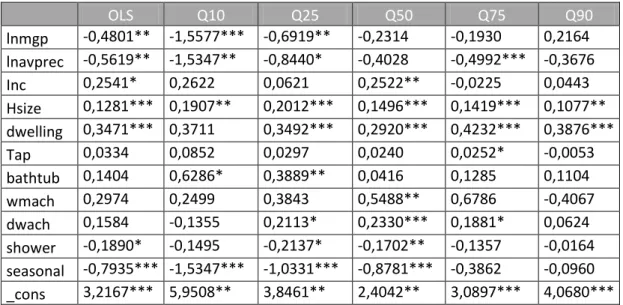
In this section we present the estimation results of the two models previously shown, one considering marginal price and the other considering average price (see Table 10 and Table 11). As exposed the dependent variable is the log monthly average water consumption of household during the 12 months starting in July 2011 and ending in June 2012. The QR models were estimated for quantiles 10, 25, 50, 75, 90. The estimated coefficients aim to measure the influence of each covariate on the whole distribution. To preserve simplicity of comparison of coefficient impacts an OLS regression is included in each table’s first column.
Table 10: Quantile regression of log water consumption on marginal price, weather and
household characteristics OLS Q10 Q25 Q50 Q75 Q90 lnmgp -0,4801** -1,5577*** -0,6919** -0,2314 -0,1930 0,2164 lnavprec -0,5619** -1,5347** -0,8440* -0,4028 -0,4992*** -0,3676 Inc 0,2541* 0,2622 0,0621 0,2522** -0,0225 0,0443 Hsize 0,1281*** 0,1907** 0,2012*** 0,1496*** 0,1419*** 0,1077** dwelling 0,3471*** 0,3711 0,3492*** 0,2920*** 0,4232*** 0,3876*** Tap 0,0334 0,0852 0,0297 0,0240 0,0252* -0,0053 bathtub 0,1404 0,6286* 0,3889** 0,0416 0,1285 0,1104 wmach 0,2974 0,2499 0,3843 0,5488** 0,6786 -0,4067 dwach 0,1584 -0,1355 0,2113* 0,2330*** 0,1881* 0,0624 shower -0,1890* -0,1495 -0,2137* -0,1702** -0,1357 -0,0164 seasonal -0,7935*** -1,5347*** -1,0331*** -0,8781*** -0,3862 -0,0960 _cons 3,2167*** 5,9508** 3,8461** 2,4042** 3,0897*** 4,0680***
Note: *Significant at 10%. ** Significant at 5%. ***Significant at 1%.. The IV standard errors have been calculated with 1000 bootstrap replications using the software package Stata 12.
26
Table 11: Quantile regression of log water consumption on average price, weather and
household characteristics OLS Q10 Q25 Q50 Q75 Q90 Lnavp -0,4218*** -1,1849*** -0,6158 -0,2340 -0,1747 -0,0914 lnavprec -0,4240*** -0,8274 -0,6060** -0,3360 -0,4486** -0,3772* Inc 0,2034** 0,1180 0,0337 0,2347** -0,0492 0,0731 Hsize 0,0889*** 0,0813 0,1354*** 0,1276*** 0,1241*** 0,1035** dwelling 0,2212*** -0,1290 0,1624 0,2264*** 0,3624*** 0,4247*** Tap 0,0207 0,0462 0,0151 0,0171 0,0221* 0,0057 bathtub 0,1954 0,4085 0,3103* -0,0101 0,1022 0,1083 wmach 0,1165 -0,2989 0,1774 0,4850* 0,5964 -0,4442 dwach 0,1726** -0,0896 0,2356** 0,2403* 0,1913* 0,0743 shower -0,1055 0,1585 -0,0880 -0,1321* -0,1041 -0,0668 seasonal -0,5401*** -0,6695*** -0,7039** -0,7230*** -0,2871 -0,2285 _cons 3,2653*** 4,8426 3,7251** 2,4662** 3,1443*** 4,0302***
Note: *Significant at 10%. ** Significant at 5%. ***Significant at 1%.. The IV standard errors have been calculated with 1000 bootstrap replications using the software package Stata 12.
Price
Marginal price
The first column of Table 10 reveals that in OLS, on average ceteris paribus, households consume less 0,48% as a response of a 1% change on marginal price. This means that demand is inelastic, as it is in literature, and a variation in price produces a smaller percentage change in the quantity of water demanded. When comparing OLS with QR regressions the change in consumption is higher in lower quantiles than in the higher ones, especially in quantile 10, where the effect is a decrease of 1,56% on the quantity of water demanded. Significance of regressions of quantiles 10 and 25 reinforce this. In that way, from the results obtained in this sample, a variation in the marginal price produces a negative and more significant impact on water consumption in those households with small consumption levels. From quantile 10 to 75, the impact gets smaller until it gets positive in quantile 90, showing an increase in consumption due to a percentage change in marginal price. Figure 3 reveals that, until quantile 30 approximately, OLS overestimates the effect of a change in price, where the opposite occurs from this quantile forward, where it underestimates it. OLS tend to send the message that all households tend to react in the same way to variations in price, QR
27
demonstrates that it is a wrong message. Households with different consumption levels tend to have different responses to the same percentage change in price.
Figure 3: The effect of marginal price
Average price
Reactions to variations in average price are expected to be negative after an increase of average price. QR estimations exposes, as marginal price estimations, that the lower consumption households respond to price increases with a great relative reduction in water consumption than higher consumption households. The effect is not constant throughout the quantiles but it is possible to see a decrease in the reaction to variations in average price from quantile 20 onwards. Although, tests of equality of quantiles are rejected, only the estimates of lower quantiles are significant (quantile 10 and 25). The effect of a percentage change in average price on household water consumption is, on average ceteris paribus, less 0,42 percentage points, when looking at the OLS estimation. The QR estimates start at a deviation of less 0,88% at the 10th quantile, and decreases a little in quantile 15, from there forward it increases to 0,02% at quantile 90. It reaches a positive variation on the 95th quantile (see Figure 3).
28
Income
From literature, households with a higher monthly net income are expected to consume more water. Although, from the QR equations one can see that it is not true. For quantile 75, which has a negative coefficient, that coefficient is not significantly different from zero. Besides OLS, only Q50 and Q95 are significant in both models A and B. Comparing now to OLS estimation, where the percentage change in the monthly net income results is a 25% or 20% percentage change (respectively for the models with marginal and average price), in the amount of water consumed by the household when comparing households with an income larger than or equal to 501€ with those that receive less than 500€ as their monthly net income.
Average precipitation
In a rainy month, households water their garden and backyards less, Tables 10 and 11 reveal that. The impact of the average precipitation is negative for the whole water consumption distribution. A one percentage change on the average precipitation results in less 0,56% in the amount of water consumed in the Model A and in Model B. It predicts a decrease in water consumption of 0,42%, on OLS. When analyzing the QR estimations it is possible to understand that the impact on Model A is the biggest and the most significant for quantile 10. For households with less net income every cent matters, so households take all opportunities to reduce their consumption in an attempt to reduce their water bill. The reverse happens to households with higher income and consumption, for whom the water bill represents a small proportion of their budget which might be a reason to explain the reduction of impact in high quantiles. Therefore, families that have a higher income tend to care less about their water consumption, so in a rainy month they probably keep watering their garden, as literature suggest. Equality tests on quantiles are rejected when comparing quantile 10 and 90, in model A. In Model B, this point does not stand out in the same way. Although all coefficients point out a negative impact on water consumption, it is not that linear. The coefficient is significant for OLS and quantiles 10, 25, 75 and 90.
29
Household size
Literature proposes that large households consume more water, which is revealed by Tables 10 and 11. More people around a dwelling predispose higher consumption levels in the sense that the household needs more water at least to bath, to cook and probably, also, to clean. Models A and B demonstrate that the household size is important for water demand estimation, not only but also, because it is significant in almost all quantiles. Household size coefficient’s values are more or less constant. Model A varies from 11% on consumption when facing an increase of one member in household, to a maximum of 20% percentage change as a result of a variation, in quantile 25. On the other hand, Model B varies from a 9% as a result of the addition of one more member to the household, in OLS, and a change of 13% on quantiles 50 and 75.
Dwelling characteristics
Dwelling characteristics are also very important when estimating water demand. When examining the type of dwelling each household lives in, it is possible to recognize that households with a detached or semi-detached dwelling have higher water consumption than those living in an apartment. Detached dwellings most of the times have backyards, gardens or pools, all characteristics that need water resulting in an increase in water consumption levels. In fact on both models, A and B, we do not see much variation in the coefficient’s values. OLS estimates in Model A that a household that lives in a detached dwelling consumes, on average ceteris paribus, more 35% than a household that lives in an apartment. When considering Model B, living in a detached house increases consumption, on average ceteris paribus, on 22% compared to apartment water consumption levels. “Dwelling” has also a great representativeness in water demand estimation as it is very significant trough quantiles.
The number of taps in a dwelling has a positive impact on water consumption levels due to an increase of one tap, as is seen in OLS where it changes by 3% in Model A and 9% in Model B. From a QR perspective, the increment of one more tap in the dwelling has
30
more expression, in both models, on the lowest quantile (Q10), valued in 9% and 5%, correspondingly. From that quantile onwards, the impact tends to decrease, reaching the point of an increment of 1%. In terms of significance, this covariate is only significant for quantile 75.
Nowadays, households tend to have either a shower or a bathtub in their dwellings. Common sense would tell us that having a shower a household consumes less water than having a bath. Is it true? From our sample, having a bathtub in the dwelling compared to not having one tends to increase water consumption and in the similar manner, in general, having a shower tends to reduce household water consumption. Common sense is verified. From OLS, in Model A, having a bathtub increases water consumption by 14% compared to those that do not have bath. And having a shower decreases water consumption by 19%. It has more impact in Q25 and Q50 compared to higher quantiles. In quantile 10, having a bathtub has more impact in water consumption than having a shower in the dwelling. In Model B, the same happens however with a small variant, in the lowest quantile having a bathtub in the dwelling has more impact than in Model A, and having a shower also increases consumption by 16% compared to those dwellings that do not have a shower.
Having a washing machine in the dwelling, from OLS Model A, increases household water consumption by 30% compared to households that do not have one. An increase of 12% on water consumption is considered in Model B. The same happens when households have a dishwasher in the dwelling; from OLS in both models it increases water consumption. Although, when looking at quantile regression in Model A, it tells us that a positive impact is in order when having one more washing machine until the 90th quantile, and that the increase in water consumption levels is higher the higher is the quantile. It varies from 25% in quantile 10 to 68% in quantile 75. On the other hand, having a dishwasher in quantile 10 it is estimated to decrease 14% water consumption compared to households that no not have a dish washer. When looking at the average price model, having a washing machine and dishwasher decreases water consumption in quantile 10, although the coefficient is not significantly different from zero. OLS gave once more the wrong idea that having a washing machine or a dishwasher would increase household water consumption. In fact it is not truth when you look at the lower consumption levels where impact is different.
31
V. Conclusions and further work
The results show that the relevant variables, price, income and weather that have been used for decades to estimate the residential water demand may have very different impacts or relevance for consumers with different consumption levels. Several explanatory variables have a lesser impact on water demand if consumption values are already large. That is the case of income, precipitation, household size, number of taps in the dwelling, the existence of a shower or a seasonal occupation of the house. Because this is also true for the consumers’ response to prices a rethinking of how the impact of a price change is computed is called for. Contrary to the common belief that higher prices in the upper blocks of the tariff are useful to promote water conservation we see that such price increases may be effective mainly in generating revenue from more rigid and large demands. It is those who already consume less that adjust their consumption the most in the face of higher marginal prices.
Further work should seek to explore more the available variables from the survey. The performed survey is very rich in information about the consumers’ characteristics and perceptions and is the first one in Portugal to combine all information about the household, the dwelling itself and the household water behaviors. There all a lot of variables that can be explored and might give interesting results, for example the behavioral questions once, as far as it is known there are no studies using Portuguese data on such theme.
The application of Quantile Regression with Instrumental Variables has some application barriers due to lack of development and software packages, but with some econometric development it is possible to go further with water demand estimation. It would be easier to test and resolve endogeneity problems and could the combination of panel data and quantile regression could be tried, something which is still very challenging right now.