A Work Project, presented as part of the requirements for the Award of a Master’s Degree in Finance from NOVA – School of Business and Economics.
PREDICTABILITY OF STOCK MARKET RETURNS – EVIDENCE FROM
EUROZONE’S BANKING SECTORS
JOÃO PEDRO DA SILVA ALMEIDA - 16000543
A Project carried out under the supervision of: Professor Miguel Ferreira
2
Abstract
This paper analyzes the in-, and out-of sample, predictability of the stock market returns
from Eurozone’s banking sectors, arising from bank-specific ratios and macroeconomic
variables, using panel estimation techniques. In order to do that, I set an unbalanced panel of 116 banks returns, from April, 1991, to March, 2013, to constitute equal-weighted country-sorted portfolios representative of the Austrian, Belgian, Finish, French, German, Greek, Irish, Italian, Portuguese and Spanish banking sectors. I find that both earnings per share (EPS) and the ratio of total loans to total assets have in-sample predictive power over
the portfolios’ monthly returns whereas, regarding the cross-section of annual returns, only
EPS retain significant explanatory power. Nevertheless, the sign associated with the impact of EPS is contrarian to the results of past literature. When looking at inter-yearly horizon returns, I document in-sample predictive power arising from the ratios of provisions to net interest income, and non-interest income to net income. Regarding the out-of-sample performance of the proposed models, I find that these would only beat the portfolios’ historical mean on the month following the disclosure of year-end financial statements. Still, the evidence found is not statistically significant. Finally, in a last attempt to find significant evidence of predictability of monthly and annual returns, I use Fama and French 3-Factor and Carhart models to describe the cross-section of returns. Although in-sample
the factors can significantly track Eurozone’s banking sectors’ stock market returns, they
3
Contents
I. Introduction ... 4
II. Explanatory Variables ... 9
III. Data and Methodology ... 14
A. Data ... 14
B. Methodology ... 17
IV. Empirical Results ... 21
A. In-Sample Results ... 21
B. Out-of-Sample Results ... 27
C. Fama and French 3-factor and Carhart Models ... 29
4
I. Introduction
This paper analyzes the in-, and out-of sample (OOS), predictability of the stock market returns from Eurozone’s constituent countries’ banking sectors, arising from bank-specific ratios and macroeconomic variables, using panel estimation techniques. In order to do that, I set an unbalanced panel of 116 banks returns, from April, 1991, to March, 2013, to constitute equal-weighted country-sorted portfolios representative of the Austrian, Belgian, Finish, French, German, Greek, Irish, Italian, Portuguese and Spanish banking sectors.
The interest of research on the banking industry relies on the fact that it is typically excluded from such empirically studies given that: firstly, when compared to other industries the sector presents abnormal high levels of leverage; secondly, given its systemic importance, there is a high level of industry-specific regulation1.
In fact, the specificities of the banking sector have already drawn the attention of academics. For instance Cooper, Jackson and Patterson (2003) constitutes a groundbreaking study on the American cross-section of banks’ stock returns, reporting evidence of in-sample (IS) predictability arising from earning per share, non-interest to net income ratio, and book value of equity to total assets ratio2. The authors also study OOS predictability, finding profitable risk-adjusted investment strategies, spanned by Boolean combinations of
1 For more on banks’ idiosyncratic characteristics see Bossone (2000).
2 The paper documents that the predictability arises from investors’ underreaction
to news. For each of the significant variables in the multivariate framework, two-way sorts are built generating positive and negative shock states based on past lagged returns. They authors exclude increased risk as a source of cross-section
predictability, by comparison of Sharpe ratios and Jensen’s alpha of the difference between the top and lowest
5
the information that arises from tercile-sorting banks with respect to each of the explanatory variables.
Although some studies explore the topic of in-sample predictability in the context of the European banking industry, the topic of OOS predictability of the banking sector is restricted to the work of Cooper, Jackson and Paterson (2003). For instance, Vennet, de Jonghe and Baele (2004) find evidence of European banking sectors’ returns’ cyclicality3, documenting predictability of book-value of equity to total assets during downturns4. Leledakis and Staikouras (2004) confirm these results, reporting also in-sample capacity of the ratio of loan loss-reserves to explain the European banks’ returns’ cross-section. More recently, Castren, Fitzpatrick and Sydow (2006) try to understand what determines
European banks’ annual stock returns, identifying dividend-related idiosyncratic
information as the main driver5.
3
The study divides the sample in two periods: before and after 2000, corresponding to an expansion and a downturn period, respectively. When country-sorting, during the expansion banks show robust positive average returns, although showing cross-country differences. Still, concordant with the hypothesis, the sample of banks present much lower average returns after 2000. Moreover, bank return reversion is higher for country portfolios that experienced the higher average return before 2000. Concerning the segment- sorting, there is a depression of average stock returns across segments from the first to the second period. The fall in average returns is more expressive for investment and commercial banks, and for non-bank credit institutions,
which the academics justify by these segments’ higher dependency from real-activity.
4 With respect to capital adequacy, as measured by the Tier 1 capital ratio or an absolute capital ratio (i.e.,
book value of equity to total assets ratio), there is a monotonic positive relation across quintiles in the economic downturn period. The effect of banking diversification, as measured by the ratio of total loans to total assets, seems to be completely inverted by the business cycle change. While during the expansion there is a negative monotonic relation across quintiles, during the economic downturn top quintiles earn higher average return. These results are ultimately confirmed by cross-section regressions against a market portfolio: better capitalized banks (top quintile), and less diversified banks (top quintile), present lower market betas.
5
6
Finally, shifting from past literature’s methodology, Drobetz, Erdmann and Zimmermann (2007) apply fixed-effects panel estimation techniques to describe the cross-section of monthly European banks’ stock returns. The authors document significant positive impact of the ratios of loans to total assets, non-interest-income to total operating income and off-balance sheet items to total assets, whereas leverage and the ratio of loan-loss provisions to net interest income affect negatively returns6.
The focus of this paper differs from past literature in three ways. Firstly, I explore the cross-sectional differences between Eurozone’s different banking sectors, as represented by banking country-specific portfolio. In this sense, the cross-section dimension is assumed to be the country of listing, as if an investor was trying to explore the variability of his country-specific banking portfolios. This differs from Vennet, de Jonghe and Baele (2004), as they only perform cross-country comparison by portfolio sorting techniques, not exploring what is on the root of the cross-country differences. Secondly, I expand the typical set of explanatory variables from only bank-specific variables, to include macroeconomic variables. As Lehmann and Manz (2006) note, the banking sector and the state of the real economy are interconnected, i.e., a stable banking system is crucial for
economic growth, but the macroeconomic environment also conditions banks’ financial
soundness and profitability. It is therefore interesting to explore if macro-related variables have predictive power over the stock market performance of Eurozone’s banking sectors. Thirdly, I go further than past European banking related studies as it is this paper’s ultimate objective to explore the OOS performance of the proposed models. Again, this differs from
6 These results differ from Leledakis and Staikouras (2004) as the study finds significant explanatory power in
7
Cooper, Jackson and Patterson (2003) as the assessment of the market-timing capacity is
performed through the models’ ability to beat the returns’ historical mean, similarly to pure
time series studies of OOS predictability.
The in-sample results show that, in fact, within the banking industry, there is evidence of stock return in-sample predictability arising from industry-specific ratios, consistent with past literature. Moreover, the fact that some bank-specific ratios are able to significantly describe the cross-section of stock returns up to 2 quarters post year-end financial
statements’ disclosure, seems to constitute evidence of investors’ underreaction to financial
information contained in year-end financial statements. This result contributes to sustain the argument that banks’ strategic and operational decisions can be tracked by industry-specific accounting ratios giving rise, differently from non-financial stocks, to in-sample stock performance predictability. Albeit with an impact contrarian to expectation, I find that only EPS can significantly describe the cross-section of monthly and annual returns, which constitutes evidence that, as with non-financial stocks, also banking stock returns can be explained by earnings related variables7.
Regarding the ability of these models to market time each of the individual banking portfolios, I find no significant evidence of OOS predictability when using monthly and annual returns. The same exercise is performed only for the month when year-end earnings’ announcement occurs. Although not statically significant, I find significant evidence that
the models’ predictions beat the monthly historical average which, once again, reinforces
7
For Instance Bauer et al. (2009) show that cash-flow-to-price ratios and earnings’ revisions are able to
8
the idea of stock return predictability arising from financial information contained in banks’ financial statements.
Finally, I use the Fama and French 3-Factor and Carhart models in a last attempt to achieve
evidence of Eurozone’s banking sectors’ stock return predictability, on a monthly and
annual basis8. Using pooled OLS estimators, I find statistically significant evidence that the Fama and French factors, with and without momentum, can contemporaneously describe
the returns’ cross-section in-sample. These results show that financial stocks, namely banking stocks, share with non-financial stocks, common risk factors. Nonetheless, I find no evidence that the factors could have been used to time each of the individual banking portfolios’ performance.
The remainder of this paper is organized as follows: Chapter II describes the set of explanatory variables used, as well as their expected relation with the cross-section of
Eurozone’s banking sectors; Chapter III describes the data as well as the econometric methodology used to explore the topic of stock return predictability; Chapter IV analyzes the empirical findings and, finally, Chapter V constitutes a brief summary of the results.
8 Fama and French (1992) show that earnings-price ratio, book-to-market ratio, leverage and size have, alone,
9
II. Explanatory Variables
In this chapter I will describe the set of explanatory variables used, exploring their expected relation with the cross-section of the individual banking sectors’ stock market return. The set of regressors includes accounting ratios and macroeconomic variables. I will first describe the bank-specific variables, and then the macroeconomic variables.
One of the advantages of dealing with banks is that the effects of their strategic and operational decisions are typically tracked in literature by a well-defined set of accounting ratios. The first used variable is the ratio of the book value of equity to total assets
(Leverage)9. This ratio should proxy a bank’s financial soundness. Still, empirical evidence on the relation of leverage and stock market performance is not conclusive. Although, Cantor and Johnson (1992) and Drobetz, Erdmann and Zimmerman (2007) document a positive relation between improving capital ratios and stock market performance, Cooper, Jackson and Patterson (2003) find the inverse.
The second variable is the percentage change in the ratio of total loans to total assets (%
Change TL/TA). This variable is a proxy to capture changes in liquidity risk: a big fraction
of a bank’s asset side is locked in long term operations, and hence a higher figure of this
ratio should reflect a less flexible balance sheet. Still, this variable should also be able to track the level of a bank’s focus on traditional operations. Although the relations seem logical, O’Hara (1993) and Santomero (1983) indicate that loan related ratios are difficultly priced, because of the level of confidentiality surrounding a bank’s loan portfolio. I
9
10
construct this variable as a percentage change given Cooper, Jackson and Patterson (2003) argument that investors react most to information reported as percentage changes. The authors have access to quarterly data and report all the banking-specific variables as percentages changes of the ratio with respect to the rolling 4-quarter mean. I do not employ this method due to its restrictive impact on the availability of observations. Still, notice that the impact of all the variables defined as percentages changes of ratios was confronted with the impact of absolute ratios, and percentage point changes, confirming the higher explanatory power of the former formulation.
In order to proxy the likelihood of future losses, the percentage change in loan loss
reserves to total loans (% Change LLR/TL) is also tested for its explanatory power over
the cross-section of returns. Contrary to the previous variable, there is much literature
documenting an adverse reaction of banks’ stock performance to increases in this figure10.
Although not commonly used in literature, one suggests that the percentage change in
provisions over net interest income (% Change Prov/NetI) should capture a bank’s
strategic decision to cover future losses with their margins arising from lending operations. Increases in this figure should mean that a bank is channeling operational income to the constitution of loan loss provisions, exemplifying precautionary action. In this sense, I expect a positive coefficient from this variable.
In order to measure the impact of banks’ hedging activities, the percentage change in
non-interest income to net income (% Change NonII/NetI)is included as explanatory variable.
10 Thakor (1987) and Lancaster, Hatfield and Anderson (1993) report that increases in the ratio of loan loss
11
Drobetz, Erdmann and Zimmermann (2007) argue that the ratio is becoming an important health indicator in the context of off balance sheet operation expansion in the banking sector. Nevertheless, the theoretical sign of the underlying relation is not consensual. On one side, there is a branch of literature suggesting that a higher stream of non-interest income is an effective hedging alternative11. On the other, it is argued that a higher dependency on non-interest income may boost risk. DeYoung and Roland (2001) argue that a higher risk pattern may arise because: firstly, usually non-interest income activities impose fixed costs’ structures resulting in higher operational leverage; secondly, it also increases financial leverage because many of these activities do not require holding regulatory capital. Cooper, Jackson and Patterson (2003) and Leledakis and Staikouras (2004) report a negative relation between this variable and the cross sections of the American and European bank returns, respectively.
The last bank specific variable is the percentage change in the efficiency ratio (% Change
ER)12. Drobetz, Erdmann and Zimmermann (2007) argue that in the context of revenues growth slowdown, banks tend to focus in cost saving initiatives, and Vennet (2002) reports that efficiency explains significantly the cross-section of European banks’ profitability. In this sense one expects a positive effect from this variable on stock returns.
11
Saunders and Walter (1994) and Grammatikos, Saunders and Swary (1986) document positive effects on
US banks’ stock performance from currency operations, whereas Gallo, Apilado and Kolari (1996) report
positive relation between mutual funds under management, as a percentage of total asset, and banking stock returns.
12 The efficiency ratio, also labeled cost to income ratio, is defined as the ratio between operational expenses
12
Apart from the described bank-specific variables, earnings per share (EPS)13 and the
book-to-market ratio (BTM) are also included as regressors. For instance, Cooper,
Jackson and Paterson (2003) and Leledakis and Staikouras (2004) report that earnings per share, and the book-to-market ratio, impact positively the cross-section of banks’ returns14.
Finally, three macroeconomic variables are included in the set of explanatory variables. The first variable is the rolling 1-year return of the 10-year German government bond
(Rf_Germany_1Y). This variable should proxy the 1 year return on a European risk-free. I do not use the one 1-year German government bond yield given that there is data available only from 1997 onwards. Still, I found a correlation between the two of about 84 percent, suggesting that estimation results should not be significantly affected by the use of a 10-year rate15.
The second variable (Risk_Prem_North) is designed to capture the impact of the pan-Eurozone sovereign movements on the banking sector, through movements in return default spread. It corresponds to the return difference between an equal weighted portfolio of 10-year government bonds of the GIPSI countries (Greece, Ireland, Portugal, Spain and Italy), and an equal weighted portfolio of the 10-year government bonds of the Central-Northern
13
Earnings correspond to earnings before extraordinary items in order to isolate one-off operations.
14
The study of impact of book-to-market differs in the two publications. Cooper, Jackson and Paterson (2003) study the impact of regression returns on the high-minus-low Fama and French factor, whereas Leledakis and Staikouras (2004) regress bank returns on their respective book-to-market ratios. Nevertheless both studies constitute evidence of the value anomaly in the banking sector.
15
13
European countries in the sample (Austria, Belgium, Finland, France and Germany)16. The recent financial crisis has delivered much evidence on the adverse reaction of stock markets to swings in European peripheral countries sovereign markets17. As such, I expect a negative impact from this variable on the banking portfolios’ returns.
The last variable is the term spread (Term_Own)18. This variable associates to each
individual portfolio its country’s spread between the 10-year government bond and a
short-term rate, as defined by the OECD19. The forecasting power of the term structure has been already studied not only in economics, regarding real activity growth, but also in finance, regarding stock market returns. To the extent that one believes that the banking sector stock market performance is linked to the evolution of real-activity, I expected a positive contemporaneous impact on returns from this variable, since term spreads are typically low around business peaks, and high around business troughs20.
Having now understood the set of explanatory variables, I will next explain how the panel
of Eurozone’s individual banking sectors is built, as well as the proposed methodology.
16 I also tested the explanatory of power of the 1-year rolling average of this variable, achieving worst results
achieving with that formulation.
17 For the impact of the Euro crisis on the European banking industry, within the framework of contagion
arising from sovereign debt markets, see Bruyckere et al. (2013).
18 As for the Risk Premium variable, I also tested the explanatory power of the 1-year rolling average,
achieving poorer results.
19
After 1999, except for Greece, the short-rate corresponds to the 3-month EURIBOR, whereas previously it
is proxied by each country’s 3-month interbank lending rate.
14
III.Data and Methodology
In this chapter I will first explain how the panel is constructed and second, describe the
models’ structure and econometric procedure used in their estimation.
A. Data
This work studies the in-, and out-of-sample, predictability using an unbalanced panel of stock returns from the Austrian, Belgian, Finish, French, German, Greek, Irish, Italian, Portuguese and Spanish banking sectors, represented by equal-weighted country-sorted portfolios21. For the portfolios formation any institution classified by Bloomberg as a bank, with a primary listing in any stock exchange of the countries above, between April, 1990, and March, 2013, is used. This requirement, combined with data availability, gives a sample of 116 banks for the composition of 10 country portfolios22.
As previously mentioned, I compare the predictive power of combinations of bank-specific ratios, market fundamentals, and macro variables. All the accounting and market data are extracted from Bloomberg database, and the macroeconomic variables from OECD database23.
Due to lack of quarterly financial statements, I use annual consolidated financial information, from 1990 up to 2011, making the assumption that full disclosure of the
21The more recent Eurozone’s
joining members (Slovenia, in 2007; Cyprus and Malta, in 2008; Slovakia, in 2009; Estonia; in 2011; and Latvia already in 2014) were not included in the database. Luxembourg and the Netherlands were excluded for data availability.
22 Data availability was a very significant constraint during this study. As such, some of the portfolios, due to
a limited number of composing banks can hardly be labeled as portfolios. This is extreme for the cases of
Ireland (1 bank), Belgium and Finland (2 banks). The remaining countries’ portfolios are composed as
follows: Austria (4 banks), France (26 banks), Germany (5 banks), Greece (8 banks), Italy (39 banks), Portugal (7 banks) and Spain (22 banks).
23 The use of OECD database for the macroeconomic is justified by the lack of long series on the used
15
annual financial statements occurs between the end of March and the beginning of April24. Moreover, all the bank-specific ratios and market fundamental variables are constructed as weighted- averages, with exception of the logarithm of market capitalization25.
Given the assumption made concerning the disclosure of financial statements, I construct an unbalanced panel of monthly returns from April, 1991, to March, 2013, and an unbalanced panel of non-overlapping annual returns (April-March), from March, 1992, to March, 2013. Apart from the two aforementioned panels, I construct 4 additional panels consisting of non-overlapping returns’ series with horizons of 1 month, and 1,2, and 3 quarters. These are assessed creating non-overlapping series of returns, for the month of April (1-Month horizon), from April to June (1-Quarter horizon), from April to September (2-Quarters horizon) and from April to December (3 Quarters-Horizon). The ranges (in parenthesis) of the different panels are as follows: 1-Month horizon (April, 1991, to April, 2012); 1-Quarter horizon (June, 1991, to June, 2012); 2-Quarters horizon (September, 1991, to September 2012); and 3-Quarters horizon (December, 1991, to December, 2012). In the case one finds that year-end financial information does not affect significantly monthly and annual returns, these panels allow the investigation of the existence of shorter time periods up to which it might. As such, one ended up with a sample of 2040 monthly-portfolio observations, and 170 non-overlapping annual; 1-month; and 1, 2 and 3-quarters
24 Similar assumptions are done by Cooper, Jackson and Paterson (2003) and Drobetz, Erdmann and
Zimmermann (2007).
25
16
portfolio observations. All returns, are measured in euros, and are adjusted for stock splits and dividends26.
Having now understood the construction of the different used panels, it is worthwhile to look at the data. For this, Appendices A and B present a descriptive summary, as well as a correlation matrix, respectively.
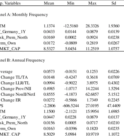
Regarding the descriptive summary in Table 1, I conclude that the cross-section of banking portfolios is far from homogeneous. I observe extreme values, especially regarding the variables that are constructed using income statement captions, namely EPS, % Change in Prov/NII and % Change NonII/NetI27. This should occur because of two facts. Firstly, the period post-2007/2008 is included in the sample representing a moment ought to give rise to extreme accounting figures in the banking sector. Secondly, as already mentioned, some of the portfolios are very idiosyncratic portfolios due to the small number of composing banks. As expected, Leverage and % Change TL/TA exhibit much higher stability.
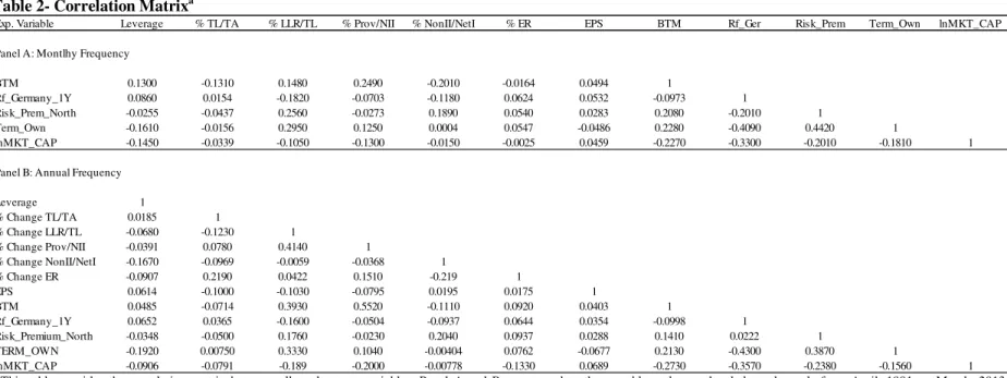
When looking at Panel B of Table 2, I draw some conclusions about the relation between the regressors. For instance the portfolios constituted by bigger banks seems to be the ones
26 As the sample combines pre- and post-euro period, all information previous to 1999 was converted to euros
at the respective fixed parity defined by each country. Alternatively to this method one could have decided to convert all information to US dollars, and introduce exchange rates as a contemporaneous control. The problem with this methodology is that it would introduce noise for the OOS estimates, since one would have
to predict foreign exchange rate movements. All individual stocks’ returns were adjusted by monthly
dividends, and I used log returns to enjoy the nice properties of additivity. Still, special attention was taken to
the fact that the log return of a portfolio is defined as ∑ , where denotes the simple
return of each portfolio’s composing stocks. 27
Given that I observe very extreme values for some variables, I have performed a robustness check for every
estimated model by comparing the estimated coefficients using the entire panels, vis-à-vis excluding from the
panels each country portfolio at a time. I repeated this procedure for every return horizon. I found that no variable either gains or loses significance, nor have I observed any coefficient changing signal. I therefore
17
financially sounder, measured by the negative correlation between the market capitalization and Leverage, % Change LLR/TL and % Change Prov/NII. Also not surprisingly, % Change Prov/NII and % Change LLR/TL are positively correlated. Interestingly enough, I also conclude that the portfolios composed of banks which are pushing harder towards operational efficiency, are exactly the ones predicting higher relative losses in their portfolio loans, as measured by the positive correlations between % Change ER and the two variables % Change Prov/NII and % Change LLR/TL.
Finally, regarding the impacts of diversification, I find evidence consistent with Drobetz, Erdmann and Zimmermann (2007): EPS is negatively correlated with % Change TL/TA and positively correlated with % Change NonII/NetI, suggesting that a deviation from traditional lending activities has been successfully impacting the flexibility of banks’
balance sheets and their earnings’ boosting capacity.
B. Methodology
In this subchapter I will explore the proposed model’s structure and estimation procedure.
Although the cross-section comparison of returns is typically performed using Fama and MacBeth (1973) cross-sectional regressions28, I use panel estimators in all models, similarly to Drobetz, Erdmann and Zimmermann (2007). The reason to use panel estimators, instead of cross-sectional regressions, relies on the results of Petersen (2007) showing that the standard errors of Fama and MacBeth (1973) methodology are downward biased in the presence of individual-effects. In order to assess the correct panel estimator I
28 Cooper, Jackson and Patterson (2003), Vennet, de Jonghe and Baele (2004), and Leledakis and Staikouras
18
run, for every model: first, the Breusche-Pagan Lagrange Multiplier test, in order to compared pooled OLS estimator with a random effects model; and second, the Wooldridge (2002) individual-effect robust expansion of the Hausman test, in order to compare the fit from a fixed-effects versus a random-effects estimator. The tests show that the fixed-effects model is the correct formulation for every estimated model. Moreover in order to check for the significance of the estimated coefficients, I use Driscoll and Kraay (1998) standard errors, as they are robust to both time and cross-sectional correlation.
Regarding the in-sample predictability I run not only a full sample estimation from April, 1991, to March, 2013, but has also split the entire sample in three periods: before the disclosure of 1998 financial statements; after the disclosure of 1999 financial statements but before the disclosure of 2007 financial statements; and lastly after the disclosure of 2007 financial statements. In the past twenty years, the countries that constitute the European Monetary Union have assisted to at least two hypothetically paradigm changing events: on one hand, obviously, the adoption of a commonly shared currency, losing the ability to conduct independent monetary policy, and booming the volume of inter-countries’ transactions; and on the other, the recent financial crisis, namely the Euro crisis, which has
been bringing to light the cracks of the Eurozone’s banking industry29. By estimating the
proposed models in the sub-samples, I examine if these events have changed the relations between the predictors and the cross-section of returns30. For every estimated model I
29
There is a vast branch of literature devoted to inter-banking contagion, and a more recent trend devoted to sovereign-banking spillovers. For more on European banking interdependence, and the effect of the Euro introduction on it, see Gropp, lo Duca and Vesala (2006), Cocozza and Piselli (2011) and OECD (2012).
30
19
condition the return in time t+1 on information up to time t, as in the context of predictive regressions31.
Also the OOS models’ market timing capacity is tested for each of the portfolios. In order to do so, I recursively estimate the fixed-effects panel model to generate, for each country-portfolio, one period-ahead forecasts, meaning that I test the ability of fixed-effects panel model to predict the individual time-series. I can interpret the process as if an investor was trying to forecast his 10 banking related portfolios’ stock market returns taking advantage of both the time-series and cross-sectional dimension of the data.
The forecasts generation is performed in two different OOS periods. The first OOS period starts after the disclosure of 1995 year-end financial statements, i.e. returns for periods after March, 1995, and goes until the end of the sample. The second OOS period is intended to check if a period of more noisy data, i.e., after the disclosure of 2007 year-end financial statements, reduced the models’ market timing capacity. As such, it begins at the same time as the first one, but goes only up to March, 2008.
In order to assess the estimated fixed-effects models’ market timing ability of each portfolio, I use the OOS as proposed by Goyal and Welch (2008):
( ), (1)
Regarding the recent financial crisis, the first turmoil in financial Markets occurred in August, 2007 with large swing in the overnight interbank lending rates, but the failure of Lehman Brother in September, 2008, is appointed as the big catalyzer of uncertainty in stock market performance. In the sense, one has modeled the financial crisis period with returns that are assumed to be dependent on year-end financial statements after 2007, i.e., returns from April, 2008, onwards.
31 Notice that for the monthly returns this means that the accounting dependent regressors are maintain fixed
20 Where the OOS is defined as:
(2)
stands for the mean square error of the one step-ahead foreacasts of the estimated models, and corresponds to the mean square error of the historical mean. I use the adjustment to the OOS suggested by Goyal and Welch (2008) as the number of regressors from the different models varies significantly, and the OOS periods for the yearly, and inter yearly, predictions are considerably small. Given this data constraint I also report the root mean square of the predictions, since there are periods for which the number of regressors is higher than the OOS observations, not allowing degrees of freedom to perform Goyal and Welch (2008) adjustment. Finally, the significance of the OOS performance is checked with the MSE-F statistic suggested by McCracken (2007):
( ), (3)
Where is set to 1 when non-overlapping returns are used, as it is this paper’s case. McCracken (2007) suggests that, in the presence of non-nested models, standard distributions can be used to assess the statistic’s significance. As one is forecasting time series with panel techniques, the individual historical mean is not nested within the estimated models, as opposed to the case of time series predictive regressions. Hence, the
21
IV.Empirical Results
I will now present the empirical results. Firstly, I will discuss the in-sample estimation results, and secondly, the OOS market timing ability of the estimated models.
A. In-Sample Results
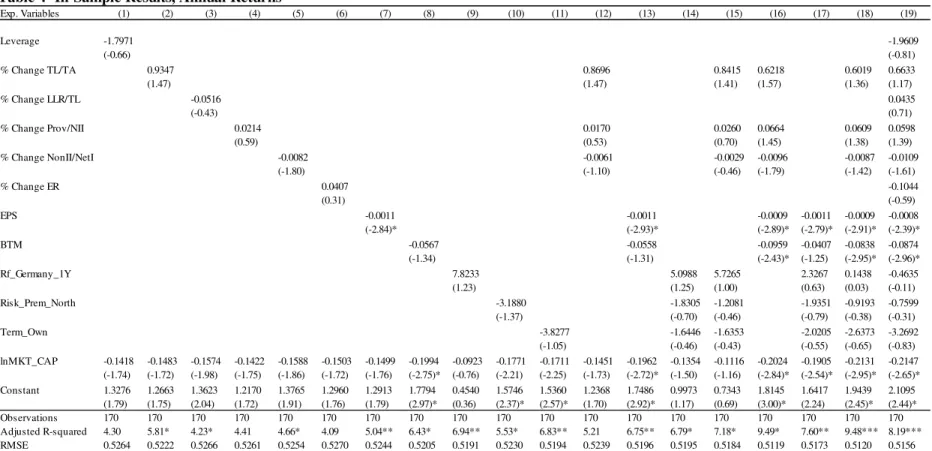
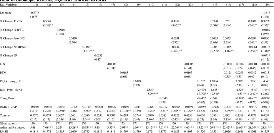
The full-sample estimations, using the monthly and non-overlapping annual returns’ panels, are shown in the Appendices C and D. I find that year-end financial statements seem to have low ability to explain monthly or annual stock market returns.
When using monthly returns only % Change TL/TA and EPS seem to have a significant impact. Regarding % Change TL/TA, it yields a positive sign, consistent with the results of Drobetz, Erdmann and Zimmermann (2007) and Leledakis and Staikouras (2004). Concerning EPS, I find a negative coefficient, which is inconsistent with the predicted sign. Moreover, when using the annual returns panel, only EPS maintains significance, similarly yielding a negative sign. The fact that EPS retains statistical significance, at least up to one year after disclosure of year-end financial statements, is consistent with Castren, Fitzpatrick
and Sydow (2006) evidence of investors’ underreaction to earnings-related information in
22
are less accurate, an information that investors tend to correct for at least one year32. In order to support this argument I would need data on earnings forecast, which one has not found.
Although not statistically significant, I still observe the relation between the remaining variables and their relation with cross-section of Eurozone’s individual banking sectors’ stock market returns. Concerning Leverage, it seems that investors penalize less sound balance sheets, consistent with Drobetz, Erdmann and Zimmermann (2007). Looking at the impact of % Change LLR/TL, it seems that increases in this figure are associated with worst annual returns. Even though the sign of the relation changes when looking at monthly returns, the magnitude of the estimator is almost zero. The proposed variable % Change Prov/NII yields the expected positive sign in both panels. Regarding the impact of revenue diversification, the results suggest that increases in % Change NonII/NetI are associated with lower average monthly and annual returns, consistent with Leledakis and Staikouras (2004). Ending with the set of bank-specific variables, increases in the operational efficiency, as measured by % Change ER, are associated with higher average monthly and annual returns, as expected.
Looking at the macroeconomic variables, I find that increases in the risk-free rate, are associated with higher returns, whereas increases in the term spread are associated with lower returns. The findings are similar for monthly and annual regressions. Although the
32 The result seems not to be driven by post-crisis noise though. When running the sub-sample estimations for
23
impact is not statistically different from zero, these relations present the opposite sign from what theory predicts. I argue that these results are related to noise arising from the period after 2007. I will return to this when analyzing the sub-sample period returns.
Concerning Risk_Prem_North, I find that it negatively impacts the market performance of
Eurozone’s individual banking sectors, as expected. Still the coefficient is not statistically
significant when using either monthly or annual returns. The fact that the coefficient of Risk_Prem_North goes in line with the expectation, when the two previous do not, may due to the fact the regressor is built as the difference in return between two sovereign portfolios, therefore presenting a smoother behavior.. These relations will be discussed below.
In order to model returns I use the ratio of book-to-market, and find that increases in the ratio are associated with worst stock market performance. This is contrarian to what the vastly documented value anomaly predicts: Socks that present higher book-to-market tend to outperform stocks with lower book-to-market. Nevertheless, the impact is not statistically different from zero. As for the logarithm of the market capitalization, used as control in every model, one finds evidence concordant with past literature, suggesting that bigger banks tend to present lower stock returns. Still, one fails to find statistically significance in the effect in most of the models.
24
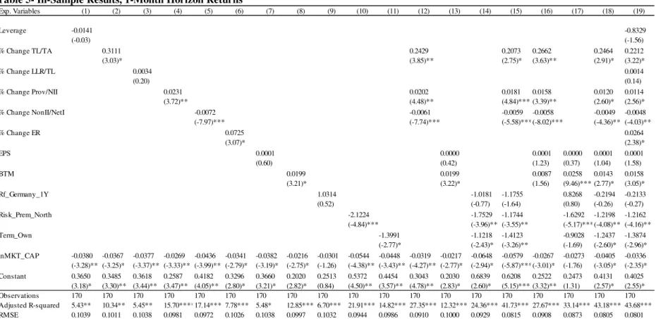
NonII/NetI and % Change ER have a statistically significant impact over the portfolios’ returns during the month following the disclosure of year-end financial statements. The sign of the impact is the same as the one achieved when running the models over the monthly, and annual panels, and the significance is maintained when combining the variables with other regressors.
Interestingly enough, EPS loses the significance when describing the cross-section of
banking sectors’ returns during the month of April. In order to see if this is because earnings information is already priced-in before announcement one has ran the same models but considering that the year-end financial statements are available between the end of February and beginning of March. When doing so, I observe a positive and significant impact of EPS on March’s Returns. Combining this piece of info with the results found using the monthly and annual returns’ panels, it seems that: first, Eurozone’s banking
sectors’ earnings are anticipated during the month of March, with investors rewarding
positively higher earnings forecasts; secondly, the movements in prices, during the month
of results’ announcements, are not related to earnings’ announcements; thirdly, after
earnings’ announcements, investors start correcting the premium they paid for earnings.
Moreover, when considering only April’s returns I find that BTM affects positively, and significantly, the returns of the individual banking sectors, consistent with the results of Drobetz, Erdmann and Zimmermann (2007) and Leledakis and Staikouras (2004). Concerning the effect of size, it is now statistically significant, maintaining the sign
25
As to the macroeconomic variables, these keep the sign observed in the previous regressions, but Term_Own and Risk_Prem_North are now statistically significant, both individually and when combined with other regressors. Notice that there is no apparent reason why these variables should significantly affect the banking monthly returns only during the month of April, but not over the entire monthly returns’ sample. I believe these findings suggest that the underlying relation is highly volatile, and is only significant in a period between 1991 and 2013. This can be shown when later looking at the sub-sample estimation results.
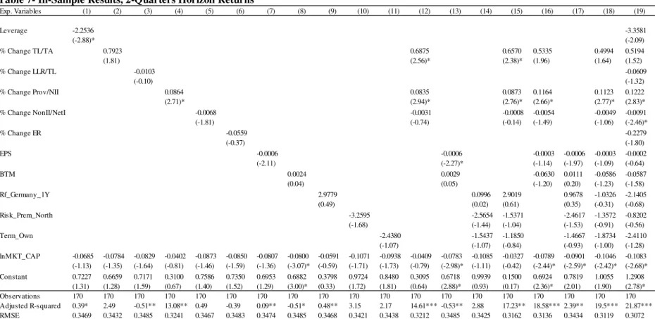
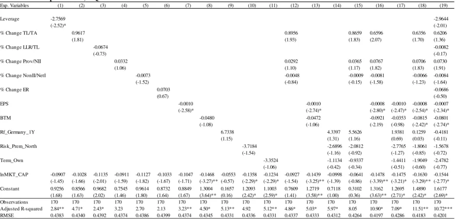
Having found a much higher number of significant regressors when describing April’s returns, than when describing the subsequent annual return, means there exists a period, between 1 month and 1 year, for which the proposed regressors can significantly describe
Eurozone’s cross-section of banking sectors’ returns. By looking at quarterly returns, one
can study the time length for which the proposed regressors retain statistically significant impacts. The estimation results for 1, 2 and 3 quarters horizon returns can be found in Appendices F to H.
26
Interesting enough, I observe that the Risk_Prem_North coefficient is negative and significant in the cross-section of Eurozone’s individual banking sectors up to 1 quarter, suggesting that investor underreact to movements in the sovereign debt markets.
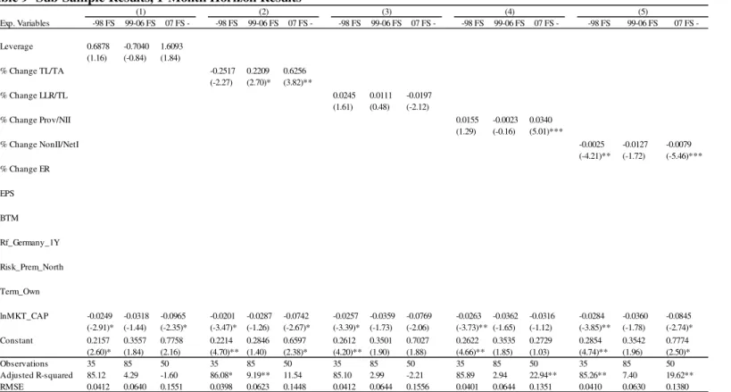
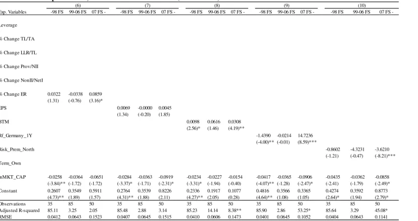
Finally, as already explained, I investigate the stability of the relations over time, running the models in three different sub-samples. I report the sub-sample estimations only using April’s returns panel, since it is the one with higher significance (See Appendix I)33.
The sub-sample regressions suggest that the bank-specific regressors’ relation with the
cross section of Eurozone’s banking sectors’ returns is not constant over time. For almost
all variables the sign of the coefficient associated with the regressor changes over periods. Still, when that occurs, the impact of the variable loses statistical significance34. This seems to correspond to the period after the Euro introduction and before the financial crisis (99-06 FS), where all the statistically significant variables either change sign, or lose significance. On the other hand, the period after 2007 (-07 FS) seems to be when all the relations between the proposed regressors gain significance, and their signs go in line with the expectations. Notice that these results are consistent with Vennet, de Jonghe and Baele (2004), if one interprets the period after the Euro introduction (99-06 FS) as a stability period, and after the financial crisis as a downturn period.
Finally, regarding the macroeconomic variables Rf_Germany_1Y and Term_Own I find a dramatic change in behavior after 2007, consistent with the argument provided to justify the
33 As once can see, by the length of Appendix D, the sub-sample estimation with the other panels is also
omitted for simplicity. Nevertheless, the same conclusions could be drawn.
34
For instance, when looking at the coefficients from % Change TL/TA, % Change Prov/NII, and % Change
NonII/NetI, I observe that the sub-periods where their coefficients’ sign change from the expectation, also
27
full in-sample estimation results achieved with those variables. Before 2007, I find the expected sign on the relation between the risk-free, and the term spread, with stock market performance.
B. Out-of-Sample Results
In this sub-chapter I will describe the results on the models’ ability to market time each of
Eurozone’s individual banking sectors. As mentioned in the methodology chapter, the OOS
performance of each model is assessed in two periods: first, from April 1996 onwards; and second, from April 1996 up to March, 2008. I present the results for the monthly, non-overlapping annual and 1-month horizon panels35.
Regarding the first OOS period, the results are shown in Appendices J and K. Not surprisingly, given the in-sample results, none of the proposed models beat the simple historical mean when estimating monthly and annual returns. Moreover, given the magnitude of the achieved out- of- sample , I conclude that the models’ predictions are extremely noisy.
When looking at Panel C, I notice that these models fail less when predicting the 1-month horizon return, given the lower RMSE of the models’ predictions. This result is consistent with the higher significance of these models’ regressors, observed in-sample, when using these returns’ panel. Still, except for the portfolio representative of the Irish banking sector, none of the models’ predictions beats the historical average. Regarding the Irish outlier, I believe the result occurs because the portfolio is the most idiosyncratic. As previously
35 Regarding the OOS for the 1-month horizon panel, one compares the models’ forecasts with the
28
mentioned, this portfolio is basically one unique stock, and so one it is not surprising that the individual mean corresponds to a very noisy predictor, easily beaten by a model that averages out the sensibility of different European banking portfolios to various regressors. As one will see in the moment, this result is driven by data after April, 2008, a period where the historical mean of an individual stock is most likely to behave very poorly as a monthly predictor, especially regarding financial groups.
When looking at the second OOS period (See Appendices L and M), I conclude that, in fact, the market timing capacity of these models is depressed by the period after the recent
financial crash. The models’ predictions RMSE is lower across all panels, when comparing
to the figures of the previous OOS period.
Although I am able to generate predictions with lower RMSE, before the disclosure of 2007 year-end financial statements, the models’ predictions are still not able to beat each
portfolio’s historical mean, when forecasting monthly and annual returns. One exception is
the French portfolio’ annual returns, where the forecasts generated using the % Change TL/TA, % Change LLR/TL, % Change Prov/NII, % Change NonII/NetI, % Change ER and EPS would have beat the historical mean. Still, the achieved figures are not statically significant. Nevertheless, it is important to remember that one is dealing with very short OOS periods where, naturally, statistical significance is difficult to achieve.
29
portfolios I find positive values for the OOS . Notice however, that the market timing accuracy during the aforementioned period varies considerably across the different
Eurozone’s banking sectors. Again, even though in same cases the OOS achieves very
impressive numbers, I conclude that these are not statistically significant.
Finally, concerning the Irish portfolio, when comparing the models’ market timing in the two OOS periods, I observe, in the latter, a lower RMSE for the models’ predictions, but also a worst OOS . Combining this piece of info, I conclude that the highly significant OOS , observed in the first period, arises from the fact that the accuracy loss in the
models’ predictions, after April, 2008, grows much less than proportionally to the accuracy
loss of prediction returns with the historical average.
So far, the evidence indicates that if the stock market performance of the individual
Eurozone’s banking sectors can in fact be timed, this occurs looking at the cross-sectional
differences in banking specific-ratios, and not at the cross-section of different reactions to macroeconomic variables. Moreover, such market timing capacity occurs only for the month in which the earnings results are disclosed to the market.
Having failed to find significant evidence of in-, and out-of-sample, predictability of monthly, and annual, returns of the Eurozone’s individual banking sectors, I repeat the exercise using the Fama and French 3-factor (FF) and Carhart models.
C. Fama and French 3-factor and Carhart Models
30
annual stock market returns. In a last attempt to achieve that goal I use the FF and Carhart models36. As before, I explore first the models’ explanatory power in-sample, and finally
try to explore the models’ ability to market time each of the individual banking, again making use of the panel estimations.
Appendix N shows the results from the in-sample estimations. I use monthly and annual contemporaneous factors to describe the monthly and non-overlapping annual excess
returns’ panels, respectively37. Moreover, instead of running fixed-effects models as before,
I use pooled OLS estimators, as identified by the Bresuch-Pagan Lagrange Multiplier test.
Regarding the full-sample estimation, I find that both models have high, and similar, explanatory power over the cross-section of Eurozone’s banking sectors’ returns. Still, the Carhart model, with the inclusion of the momentum factor (WML), seems to slightly better fit the data. When using the models to explain monthly returns (Panel A of table 17), all regressors are highly significant except the Small-minus-Big factor (SMB). That result changes regarding annual returns (Panel B of table 17), where the SMB changes sign and becomes statistically significant when running the Carhart model.
In order to explore the consistency in the models’ explanatory power over time, I divide the
sample in the same three previously used periods. The results in table 18 indicate that the
relation between the factors and Eurozone’s banking sectors’ returns has not been constant
36One uses Fama and French’s European Factors, extracted from Kenneth French’s website:
http://mba.tuck.dartmouth.edu/pages/faculty/ken.french/data_library.html#International.
37
Regarding the annual factors, Kenneth French’s dataset includes annual factors, where the annual returns
are measured from January to December of each year. As the used panel starts in April, one makes uses of the
monthly factors to compute each factor’s 12-month compounded return, from April to March. Concerning the
excess returns, these were computed using the risk-free available in Kenneth French’s database. For the
31
over time. Moreover, the models’ explanatory power has been growing with time. I argue
that this indicates a higher synchronism between the individual banking sectors. Notice that, the pooled OLS estimation is imposing the same betas for all the individual portfolios in a context where we are not allowing for individual effects. In this sense, better figures for the in-sample indicate that the individual portfolios’ reaction to these common factors has been becoming more similar.
Having found that both the Fama and French 3-Factor and Carhat’s models can describe the cross-section of Eurozone’s banking sectors monthly and annual excess returns, I try, as before, to see if the models could be used to market time the individual banking portfolios, in the two previously considered OOS periods. Notice that, to do so, I had to adjust the
models’ structures, conditioning the portfolios’ excess returns in time t+1 on the factors’ returns at time t. Moreover, as the models forecast excess returns for time t+1, I add up the risk-free rate available at time t, in order to have an estimate of the effective return at time t+1. Finally, in order to check if the factors forecasting ability is reduced by the possibility that the portfolios’ individual betas are very heterogeneous, I model, individually, each
portfolio’s monthly and annual excess return for forecasting purposes, i.e., using time series
techniques38. In order to start recursively estimating the individual time-series models I only require 3 years of data.
38 Notice that in the context of time-series predictive regressions, MacCraken (2007) proposed MSE-F
statistic, used to determine the statistical significance of Goyal and Welch (2008) OOS , cannot anymore be
assessed using standard distributions, as the portfolio’s historical mean is nested within the used models. In
this case, MacCraken(2007) proposes the use of bootsrapped critical values. Still, one has not worried with
32
Appendices O and P show the results. As before, I fail to find any evidence of OOS predictability. I find no positive OOS in any of the two periods, indicating that, for market-timing purposes, the historical mean has outperformed the models’ forecasts. Still, as before, when I truncate the OOS period to March, 2008, the RMSE of the models’ predictions improve.
Lastly, I also conclude that the used factors’ lack of accuracy to forecast the portfolio’s monthly and annual returns is not driven by the fact one is not modelling individually the
portfolio’s returns with Fama and French 3-Factor and Carhart models. In fact, the
estimates from the individual time-series present worse RMSE, which is due to the fact the models are estimated with much less data. This can been seen by the fact that the
discrepancies in the predictions’ RMSE are bigger for the banking portfolios that present
less available data, namely the Austrian, Belgian, Finnish, Greek and Irish portfolios.
This last analysis ends the set of achieved results when describing Eurozone’s banking
sectors’ monthly and annual returns with Fama and French factors.
V. Conclusions
33
sectors’ monthly and non-overlapping annual (April-March) returns’ from April, 1991, to
March, 2013.
Regarding the monthly returns panel, I find that both EPS and the ratio of total loans to total assets have in-sample predictive power whereas, concerning the cross-section of annual returns, only EPS has significant explanatory power. Nevertheless, the sign associated with the impact of EPS is contrarian to the results of past literature. I argue that the result may occur if the banking sectors presenting higher earnings, are also those where earnings’ estimates are less accurate.
Failing to find an expressive number of significant regressors to describe the cross-section of monthly and annual returns, I explore the in-sample predictability of the set of variables over the month following the disclosure of year-end financial statements, and also past 1, 2 and 3 quarters. When performing this exercise I find that the ratios of non-interest income to net income, and provisions to net interest income have predictive power over Eurozone’s
banking sectors’ returns up to 1 and 2 quarters, respectively, after disclosure of year-end figures.
The in-sample results show that, in fact, within the banking industry, there is evidence of in-sample stock return predictability arising from industry-specific ratios, consistent with past literature. Moreover, the fact that some bank-specific ratios are able to significantly describe the cross-section of stock returns up to 2 quarters post year-end financial
statements’ disclosure, seems to constitute evidence of investors’ underreaction to financial
34
argument that banks’ strategic and operational decisions can be tracked by industry-specific
accounting ratios giving rise, differently from non-financial stocks, to in-sample stock performance predictability.
Regarding the ability of these models to market time each of the individual banking portfolios, I find no significant evidence of OOS predictability when using monthly and annual returns. The same exercise is performed only for the month when year-end earnings’ announcement occurs. Although not statically significant, I find significant evidence that
the models’ predictions beat the monthly historical average which, once again, reinforces
the idea of stock return predictability arising from financial information contained in banks’
financial statements.
Finally, I use the Fama and French 3-Factor and Carhart models in a last attempt to achieve
evidence of Eurozone’s banking sectors’ stock return predictability, on a monthly and
35
References
Bauer, Rob; Diris, Bart F.; Pavlov, Borislav and Schotman, Peter C. 2009. “Firm
Characteristics, Industry, Horizon and Time Effects, in the Cross-Section of Expected
Stock Returns.” University of Maastricht, Limburg Institute of Financial Economics,
Working Paper.
Bossone, Biagio. 1999. "What Makes Banks Special? A Study of Banking, Finance, and
Economic Development." The World Bank, Policy Research Working Paper Series: 2408.
Campbell, John Y. and Motohiro Yogo. 2006. "Efficient Tests of Stock Return
Predictability." Journal of Financial Economics, 81(1): 27-60.
Cantor, Richard and Ronald Johnson. 1992. "Bank Capital Ratios, Asset Growth, and
the Stock Market." Federal Reserve Bank of New York Quarterly Review, 17(3): 10-24.
Carhart, Mark M. 1997. "On Persistence in Mutual Fund Performance." Journal of
Finance, 52(1): 57-82.
Castren, Olli; Trevor Fitzpatrick and Matthias Sydow. 2006. "What Drives Eu Banks'
Stock Returns? Bank-Level Evidence Using the Dynamic Dividend-Discount Model." European Central Bank, Working Paper Series: 677.
Cooper, Michael J.; William E. Jackson, III and Gary A. Patterson. 2003. "Evidence of
36
De Bruyckere, Valerie; Maria Gerhardt; Glenn Schepens and Rudi Vander Vennet.
2013. "Bank/Sovereign Risk Spillovers in the European Debt Crisis." Journal of Banking and Finance, 37(12): 4793-809.
DeYoung, Robert and Karin P. Roland. 2001. "Product Mix and Earnings Volatility at
Commercial Banks: Evidence from a Degree of Total Leverage Model." Journal of Financial Intermediation, 10(1): 54-84.
Drobetz, Wolfgang; Thomas Erdmann and Heinz Zimmermann. 2007. "Predictability
in the Cross-Section of European Bank Stock Returns." Universität Basel, Wirtschaftswissenschaftliches Zentrum, Working Paper.
Fama, Eugene F. 1990. "Stock Returns, Expected Returns, and Real Activity." Journal of
Finance, 45(4): 1089-108.
Fama, Eugene F. and Kenneth R. French. 1992. "The Cross-Section of Expected Stock
Returns." Journal of Finance, 47(2): 427-65.
Fama, Eugene F. and Kenneth R. French. 1993. "Common Risk Factors in the Returns
on Stocks and Bonds." Journal of Financial Economics, 33(1): 3-56.
Fama, Eugene F. and James D. MacBeth. 1973. "Risk, Return, and Equilibrium:
Empirical Tests." Journal of Political Economy, 81(3): 607-36.
Gallo, John G.; Vincent P. Apilado and James W. Kolari. 1996. "Commercial Bank
Mutual Fund Activities: Implications for Bank Risk and Profitability." Journal of Banking and Finance, 20(10): 1775-91.
Goval, Amit and Ivo Welch. 2004. "A Comprehensive Look at the Empirical Performance
37
Grammatikos, Theoharry; Anthony Saunders and Itzhak Swary. 1986. "Returns and
Risks of U.S. Bank Foreign Currency Activities." Federal Reserve Bank of Philadelphia, Working Papers: 86-2.
Gropp, Reint; Marco Lo Duca and Jukka Vesala. 2006. "Cross-Border Bank Contagion
in Europe." European Central Bank, Working Paper Series: 662.
Lancaster, Carol; Gay Hatfield and Dwight C. Anderson. 1993. "Stock Price Reactions
to Increases in Loan-Loss Reserves: A Broader Perspective." Journal of Economics and Finance, 17(3), 29-41.
Leledakis, George and Christos Staikouras. 2004. "The Stock Return Predictability of
the European Banking Sector Working Paper," Athens University of Economics and Business, Working Paper.
Lehmann, Hansjorg and Michael Manz. 2006. "The Exposure of Swiss Banks to
Macroeconomic Shocks - an Empirical Investigation," Swiss National Bank, Working Papers: 2006-04.
McCracken, Michael W. 2007. "Asymptotics for out of Sample Tests of Granger
Causality." Journal of Econometrics, 140(2): 719-52.
OECD. 2012. "Financial Contagion in the Era of Globalised Banking?" OECD Economics
Department Policy Notes: 14.
O'Hara, Maureen. 1993. "Real Bills Revisited: Market Value Accounting and Loan
Maturity." Journal of Financial Intermediation, 3(1): 51-76.
Santomero, Anthony M. 1983. "Fixed Versus Variable Rate Loans." Journal of Finance,
38
Saunders, Anthony and Ingo Walter. 1994. Universal Banking in the United States:
What Could We Gain? What Could We Lose? New York; Oxford; Toronto and Melbourne:
Oxford University Press.
Thakor, Anjan V. 1987. "Discussion." Journal of Finance, 42(3): 661-63.
Vennet, Rudi Vander. 2002. "Cost and Profit Efficiency of Financial Conglomerates and
Universal Banks in Europe." Journal of Money, Credit & Banking (Ohio State University Press), 34(1): 254-82.
Vennet, Rudi Vander; Olivier De Jonghe and Lieven Baele. 2004. "Bank Risks and the
Business Cycle." University of Ghent, Working Paper Series: 4264.
Wooldridge, Jeffrey M. 2002. Econometric Analysis of Cross Section and Panel Data.
39
Appendix A
Table 1- Descriptive Statisticsa
a This table provides the Mean, Min, Max and Standard Deviation for all the explanatory variables. Panel A and B correspond to the
monthly and annual unbalanced panels from April, 1991, to March, 2013, respectively. The descriptive statistics for the bank-specific are omitted in Panel A because are based in annual data. Leverage corresponds to the ratio of the book value of equity to total assets; % Change TL/TA corresponds to the percentage change of the ratio of total loans to total assets; % Change LLR/TL corresponds to the percentage change of the ratio of loan loss reserves to total loans; % Change Prov/NII corresponds to the percentage change of the ratio of provisions to net interest income; % Change NonII/NetI corresponds to the percentage change of the ratio of non-interest income to net income; % Change ER corresponds to the percentage change of the efficiency ratio; EPS corresponds to the earnings per share ratio; BTM corresponds to the book-to-market ratio; Rf_Germany_1Y corresponds to the rolling 1-year return on the 10-year German government bond; Risk_Prem_North, corresponds to the return difference between the an equal weighted portfolio of 10 -year government bonds of Portugal, Ireland, Greece, Spain and Italy, and an equal weighted portfolio of 10-year government bonds of Austria, Belgium, Finland, France and Germany; and Term_Own corresponds to individual-specific difference between the 10-year government bond yield and the 3-month interbank lending rate.
Exp. Variables Mean Min Max Sd
Panel A: Monthly Frequency
BTM 1.1374 -12.5160 28.3326 1.9360 Rf_Germany_1Y 0.0433 0.0144 0.0879 0.0139 Risk_Prem_North 0.0169 0.0002 0.0924 0.0238 Term_Own 0.0172 -0.0809 0.2819 0.0267 lnMKT_CAP 8.5327 5.0454 11.2519 1.0757
Panel B: Annual Frequency
Leverage 0.0573 -0.0151 0.1253 0.0226 % Change TL/TA 0.0148 -0.4247 0.3618 0.0769 % Change LLR/TL 0.0994 -0.9022 3.8975 0.4302 % Change Prov/NII 0.4985 -1.0717 14.2244 1.5294 % Change NonII/NetI 0.8555 -4.1873 62.6857 5.1512 % Change ER 0.0272 -0.5866 1.7349 0.2245 EPS -2.2806 -606.5244 27.0195 47.4409
BTM 1.1500 -2.1121 15.9954 1.6985
40
Appendix B
Table 2- Correlation Matrixa
a This table provides the correlation matrix between all explanatory variables. Panel A and B correspond to the monthly and annual unbalanced panels from April, 1991, to March, 2013,
respectively. The descriptive statistics for the bank-specific are omitted in Panel A because are based in annual data. Horizontal variable names are shortened for better fitting. Leverage corresponds to the ratio of the book value of equity to total assets; % Change TL/TA (%TL/TA) corresponds to the percentage change of the ratio of total loans to total assets; % Change LLR/TL (%LLR/TL) corresponds to the percentage change of the ratio of loan loss reserves to total loans; % Change Prov/NII (% Prov/NII) corresponds to the percentage change of the ratio of provisions to net interest income; % Change NonII/NetI (%NonII/NetI) corresponds to the percentage change of the ratio of non-interest income to net income; % Change ER (% ER) corresponds to the percentage change of the efficiency ratio; EPS corresponds to the earnings per share ratio; BTM corresponds to the book-to-market ratio; Rf_Germany_1Y corresponds to the rolling 1-year return on the 10-year German government bond; Risk_Prem_North, corresponds to the return difference between the an equal weighted portfolio of 10-year government bonds of Portugal, Ireland, Greece, Spain and Italy, and an equal weighted portfolio of 10-year government bonds of Austria, Belgium, Finland, France and Germany; and Term_Own corresponds to individual-specific difference between the 10-year government bond yield and the 3-month interbank lending rate.
Exp. Variable Leverage % TL/TA % LLR/TL % Prov/NII % NonII/NetI % ER EPS BTM Rf_Ger Risk_Prem Term_Own lnMKT_CAP
Panel A: Montlhy Frequency
BTM 0.1300 -0.1310 0.1480 0.2490 -0.2010 -0.0164 0.0494 1
Rf_Germany_1Y 0.0860 0.0154 -0.1820 -0.0703 -0.1180 0.0624 0.0532 -0.0973 1
Risk_Prem_North -0.0255 -0.0437 0.2560 -0.0273 0.1890 0.0540 0.0283 0.2080 -0.2010 1
Term_Own -0.1610 -0.0156 0.2950 0.1250 0.0004 0.0547 -0.0486 0.2280 -0.4090 0.4420 1
lnMKT_CAP -0.1450 -0.0339 -0.1050 -0.1300 -0.0150 -0.0025 0.0459 -0.2270 -0.3300 -0.2010 -0.1810 1
Panel B: Annual Frequency
Leverage 1
% Change TL/TA 0.0185 1
% Change LLR/TL -0.0680 -0.1230 1
% Change Prov/NII -0.0391 0.0780 0.4140 1
% Change NonII/NetI -0.1670 -0.0969 -0.0059 -0.0368 1
% Change ER -0.0907 0.2190 0.0422 0.1510 -0.219 1
EPS 0.0614 -0.1000 -0.1030 -0.0795 0.0195 0.0175 1
BTM 0.0485 -0.0714 0.3930 0.5520 -0.1110 0.0920 0.0403 1
Rf_Germany_1Y 0.0652 0.0365 -0.1600 -0.0504 -0.0937 0.0644 0.0354 -0.0998 1
Risk_Premium_North -0.0348 -0.0500 0.1760 -0.0230 0.2040 0.0937 0.0288 0.1410 0.0222 1
TERM_OWN -0.1920 0.00750 0.3330 0.1040 -0.00404 0.0762 -0.0677 0.2130 -0.4300 0.3870 1