Date of publication xxxx 00, 0000, date of current version xxxx 00, 0000.
Digital Object Identifier 10.xxxx/ACCESS.20xx.DOI
Distribution of the Residual
Self-Interference Power in In-Band
Full-duplex Wireless Systems
LUIS IRIO1,2, RODOLFO OLIVEIRA1,2, (Senior Member, IEEE) 1Instituto de Telecomunicações, 1049-001 Lisbon, Portugal
2Departamento de Engenharia Electrotécnica, Faculdade de Ciências e Tecnologia, FCT, Universidade Nova de Lisboa, 2829-516 Caparica, Portugal
Corresponding author: Luis Irio ([email protected]).
This work was supported by the Project CoSHARE (LISBOA-01-0145-FEDER-0307095 - PTDC/EEI-TEL/30709/2017), Project UID/EEA/50008/2019, grant SFRH/BD/108525/2015, in part by the Fundo Europeu de Desenvolvimento Regional (FEDER), through Programa Operacional Regional LISBOA (LISBOA2020), and by the national funds, through Fundação para a Ciência e Tecnologia (FCT).
ABSTRACT This work derives the distribution of the residual self-interference power in an analog post-mixer canceler adopted in a Wireless In-Band Full-Duplex communication system. We focus on the amount of uncanceled self-interference power due to self-interference channel estimation errors. Closed form expressions are provided for the distribution of the residual self-interference power when Rician and Rayleigh fading interference channels are considered. Moreover, the distribution of the residual self-interference power is derived for low and high channel gain dynamics, by considering the cases when the self-interference channel gain is time-invariant and time-variant. While for time-invariant channels the residual self-interference power is exponentially distributed, for time-variant channels the exponential distribution is not a valid assumption. Instead, the distribution of the residual self-interference power can be approximated by a product distribution. Several Monte Carlo simulation results show the influence of the channel dynamics on the distribution of the residual self-interference power. Finally, the accuracy of the theoretical approach is assessed through the comparison of numerical and simulated results, which confirm its effectiveness.
INDEX TERMS In-band full-duplex Radio Systems, Residual Self-interference Power, Stochastic Model-ing, Performance Analysis.
I. INTRODUCTION
Current wireless communication systems, including but not limited to cellular and local area networks, are half-duplex communication systems, meaning that the available re-sources are divided either in time domain or in frequency do-main. Consequently, transmission and reception occur either at different times or in different frequency bands. Recently, a different approach has been investigated where the wireless terminals transmit and receive simultaneously over the same frequency band [1]–[3], which is known as In-Band Full Duplex (FDX) communications [4], [5].
By using FDX communications, the capacity of the com-munication link may be increased up to twice the amount of half-duplex communication systems [6]–[8]. However, to simultaneously transmit and receive, a terminal must separate its own transmission from the received signal, which is usu-ally referred to as self-interference cancellation (SIC), posing
several challenges at different levels, ranging from circuit design to signal processing.
The success of FDX communications relies on the per-formance of SIC schemes. Since the transmitted signal may suffer different propagation effects, a terminal cannot simply cancel self-interference (SI) by subtracting its transmitted signal from the received one. Rather, digital-domain cancel-lation (DC) must be employed to account for the estimated effects of the propagation channel [9], [10]. But it is well known that DC is unable to completely suppress the SI [11]. Consequently, the SI is usually reduced before the DC through the adoption of an analog-domain cancellation (AC) technique [12], [13]. By using the two types of cancellation, the channel unaware AC technique suppresses a significant amount of direct-path SI, while the channel aware DC tech-nique may suppress the remaining SI [14].
self-interference power in an analog post-mixer canceler, which represents the amount of uncanceled self-interference due to imperfect self-interference channel estimation and imperfections in the transmission chain [11]. Closed form expressions are derived for the distribution of the residual self-interference power when Rician and Rayleigh fading self-interference channels are considered. The distribution of the residual self-interference power is also derived for low and high channel gain dynamics, by considering the cases when the self-interference channel gain is time-invariant and time-variant. Finally, we present different simulation results to show the influence of the channel dynamics on the dis-tribution of the self-interference power. The accuracy of the proposed methodology is also evaluated for the limit case, when the frequency of the signal to transmit approaches the carrier frequency.
The rest of the paper is organized as follows. Next we review relevant research works related with the design and analysis of In-Band Full Duplex communication systems. Section II introduces the assumptions made regarding the system model. Section III describes the steps involved in the theoretical characterization of the residual SI power. The accuracy of the proposed methodology is evaluated in Sec-tion IV, where numerical results computed with the proposed model and Monte Carlo simulation results are compared. Finally, Section V concludes the paper by outlining its con-tribution.
Notations: In this work, fX(.) and FX(.) represent the
probability density function (PDF) and the cumulative dis-tribution function (CDF) of a random variable X, respec-tively. (.) denotes the Dirac’s delta function. (.) represents the complete Gamma function. Kv(.)denotes the modified
Bessel function of the second kind with order v. N (µ, ) represents a Gaussian random variable with mean µ and variance . Gamma(k, ✓) denotes a Gamma distribution with a shape parameter k and a scale parameter ✓. Exp( ) denotes a Exponential distribution with rate parameter and 2
1
rep-resents a chi-squared distribution with 1 degree of freedom.
A. RELATED WORK
In FDX communications, the transmitter’s (TX) signal must be reduced to an acceptable level at the receiver (RX) located in the same node. Any residual SI will increase the RX noise floor, thus reducing the capacity of the RX channel. FDX communications’ performance is limited by the amount of SI suppression, which may be achieved by two different methods:
• Antenna Isolation (AI) [15], [16], to prevent the
RF-signal generated by the local TX from leaking onto the RX;
• Self-interference Cancellation (SIC) [9], [10], [13], to
subtract any remaining SI from the RX path using knowledge of the TX signal and channel estimation. AI is fundamentally limited by the physical separation of the antennas [16]. The SIC performance depends on the
ac-curacy with which the transmitted signal can be copied, mod-ified and subtracted. The signal to be subtracted is usually a modified copy of the transmitted one, obtained by a simulated channel path between the points where signals are sampled and subtracted. Three different active SIC architectures are reported in the literature:
• Analog-domain cancellation [17], [18]; • Digital-domain cancellation [4], [9], [19]; • Mixed-signal cancellation (MXC) [20]–[22].
AC schemes can provide up to 40-50 dB cancellation [18], exhibiting higher performance than DC. This is explained by the fact that the cancellation signal includes all TX im-pairments, and it relaxes requirements further downstream. However, it requires processing the cancellation signal in the analog RF domain, increasing hardware costs and complex-ity. AC cancellation can be done either at the analog baseband or at the carrier radio-frequency (RF). The cancelling signal may be generated by processing the SI signal prior to the up-conversion stage (pre-mixer cancellers), or after the SI signal being upconverted (post-mixer cancellers). In both cases, the performance is limited by the phase noise of the oscillators used in the up/down conversion [20], [23]. AC presents several challenges, which may include the non-linear effects of power amplifiers [11], [24], the In-phase/Quadrature (IQ) imbalance [24], [25], and the phase noise of both transmitter and receiver [23], [26], [27].
In DC schemes the signals are processed in the digital domain, making use of all digital benefits, including the SI wireless channel awareness, through adequate channel estimation techniques. However, DC cannot remove the SI in the analog RX chain, being unable to prevent the analog circuitry to block the reception due to nonlinear distortion or the ADCs’ quantization error [28]. It is well known that DC is unable to completely suppress the SI, mainly because the dynamic range of the analog-to-digital converters (ADC) limits the amount of suppressed SI, due to the limited effective number of bits (ENOB) [11], [29]. Commercial ADCs have improved significantly in sampling frequency but only marginally in ENOB. DC can provide up to 30-35 dB cancellation in practice [30], being limited by a noisy estimate of the SI channel and noisy components of the self-interferer that cannot be cancelled [31], [32].
In MXC schemes, both AC and DC are considered. The digital TX signal is processed and converted to analog radio-frequency (RF), where subtraction occurs [20], [21], and it is processed after the AC [20], [22]. This requires a dedi-cated additional upconverter, which limits the cancellation of current MXC schemes to 35 dB [20]. To achieve overall SI suppression close to 100 dB above the noise floor, both AC and DC must be used in a MXC scheme.
The residual SI is mainly due to estimation errors oc-curring during the time domain cancellation [28], and has been addressed in various works in the literature [11], [33]– [39]. [11] has identified the quantization-noise, the phase-noise in the local oscillator, and the channel estimation error, as being the main causes of incomplete self-interference
cancellation in different FDX schemes. [33] analyzed the impact of the phase-noise on the distribution of the residual SI power, showing that the phase-noise is almost negligible when the oscillators’ phase-noise is close to the minimum achievable phase noise of RC oscillators [40]. However, we highlight that the conclusions in [33] are only based on simulations without any theoretical understanding. [34] has analyzed nonlinear distortion effects occurring in the trans-mitter power amplifier and also due to the quantization noise of the ADCs at the receiver chain. The uncertainty associated with the residual self interference channel was studied in [35], which has proposed a block training scheme to estimate both communication and residual SI channels in a two-way relaying communication system. The residual SI channel was also studied in [36], showing that the channel can be modeled as a linear combination of the original signal and its derivatives. The authors adopt a Taylor series approximation to model the channel with only two parameters, and a new SI cancellation scheme based on the proposed channel model is also described. [37] investigates the detrimental effects of phase noise and in-phase/quadrature imbalance on full-duplex OFDM transceivers, showing that more sophisticated digital-domain SI cancellation techniques are needed to avoid severe performance degradation. [37] derives a closed-form expression for the average residual self-interference power and describes its functional dependence on the parameters of the radio-frequency impairments. The residual SI is also characterized in [38] for a multi-user input multiple-output (MIMO) setup considering FDX multi-antenna nodes and assuming the availability of perfect channel state infor-mation. The authors show that for the MIMO scenario the residual SI can be approximated by a Gamma distribution assuming time-invariant channels. [39] investigated if the residual SI power can be accurately approximated by known distributions. The paper shows that Weibull, Gamma and Exponential distributions fail to approximate the residual SI power in an accurate way. This observation was only based on Monte Carlo simulation results, from which the parameters of the known distributions were obtained using a fitting tool based on the Maximum Likelihood Estimation method. The results in [39] have motivated us to derive the distribution of the residual SI power in a theoretical way, which is the main topic addressed in this paper.
B. CONTRIBUTIONS
Motivated by the importance of the analog SI’s characteri-zation in the joint cancellation process, this work derives a theoretical analysis of the residual SI power, i.e., the amount of uncanceled self-interference due to channel estimation errors at the analog cancellation process. The proposed anal-ysis neglects the nonlinear effects due to RF impairments (e.g. ADCs and power amplifier impairments), although the impact of the phase noise is analyzed through Monte Carlo simulation results. We believe that our work is a first step to derive more complex models, as nonlinear effects can be modeled as a linear combination of multiple input signals
[36].
To the best of the authors’ knowledge, this is the first work deriving the distribution of the residual self-interference power in an analog post-mixer canceler scheme. The results and the insights presented in this work are new and can definitely be used as a benchmark for future studies. Our contributions are as follows:
• We derive closed form expressions for the distribution of
the residual SI power when Rician and Rayleigh fading self-interference channels are considered;
• The impact of the fading channel is evaluated on
the distribution of the residual SI power and the re-sults achieved confirm that the type of fading chan-nel strongly impacts the distribution of the residual SI power;
• The distribution of the residual SI power is derived for
low and high channel gain dynamics, showing that the channel dynamics strongly influences the distribution of the self-interference power;
• Numerical results computed with the proposed model
are compared with Monte Carlo simulation results to evaluate the accuracy of the theoretical analysis for both SI channel’s gain and phase estimation errors;
• The accuracy of the theoretical analysis is also assessed
for the limit case when the frequency of the input signal to be transmitted is close to the carrier frequency. In this way we identify the dynamic region where the proposed approach achieves high accuracy;
• The impact of the phase noise is evaluated through
Monte Carlo simulation results for different values of phase noise variance.
The need of analog and digital-domain cancellation re-quires a precise characterization of the amount of interfer-ence not canceled in the analog-domain. The knowledge of the residual SI due to the AC is crucial to design efficient SI estimation methods to be used in the digital-domain. By doing so, the efficiency of the joint AC and DC schemes may be improved.
II. SYSTEM MODEL
In this work we consider a full-duplex scheme adopting an active analog canceler that reduces the self-interference at the carrier frequency. The active analog canceler actively reduces the self-interference by injecting a canceling signal into the received signal. A post-mixer canceler is assumed, because the canceling signal is generated by processing the self-interference signal after the upconversion stage [23]. The block diagram of the system model is shown in Fig. 1.
The self-interference signal xsi(t)is up-converted to the
frequency !c = 2⇡fc and transmitted over the full-duplex
channel characterized by the gain h and the delay ⌧. In this work we consider that the active analog canceler estimates the channel’s gain and delay in order to reduce the residual self-interference yrsi(t).
FIGURE 1: Block diagram representation of the post-mixer canceller.
The residual self-interference, yrsi(t), is represented as
follows
yrsi(t) = xsi(t)e
j!ct
⇤ hsi(t) xsi(t)ej!ct⇤ ˆhsi(t), (1)
where xsi(t)is the SI signal, hsi(t)is the impulse response
of the SI channel, ˆhsi(t) represents the estimate of the SI
channel, !c is the angular frequency and ⇤ represents the
convolution operation. The SI channel considered in our work is a single-tap delay channel, i.e., hsi(t) = h (t ⌧ ).
Similarly, the estimate of the SI channel is denoted by ˆ
hsi(t) = hc (t ⌧c), where hcand ⌧care the estimated SI
channel’s gain and delay, respectively.
We assume that the SI signal, xsi(t), is a
circularly-symmetric complex signal, representing the case when Or-thogonal Frequency-Division Multiplexing with a high num-ber of sub-carriers is adopted [41]. Departing from the resid-ual SI in (1), it can be rewritten as
yrsi(t) = h xsi(t ⌧ )e
j(!c(t ⌧ ))
hcxsi(t ⌧c)ej(!c(t ⌧c)).
(2) In what follows we consider that the channel gain is complex, h = hr+ jhj, and the estimate of the channel’s gain is given
by hc = ✏h, where (1 ✏)is the channel’s gain estimation
error. Channel’s phase estimation error is represented by = !c(⌧ ⌧c). We also consider that the SI signal xsi(t)is
a random signal, whose value for a specific sample k is repre-sented by a pair of two random variables (RVs) {Xr, Xj}, i.e.
for a specific sample k we represent xsi(k T) = Xr+ jXj,
where T represents the sample period. If the sample period
is low, i.e. T << 2⇡/!c, and the value of the RVs Xr+jXj
remain constant for several samples, we may assume that Pr[xsi(t ⌧ ) xsi(t ⌧c) = 0]is high, since the SI signal
xsi(k T)may remain constant for a consecutive number of
samples1. After a few algebraic manipulations, the residual
SI can be represented by its real and imaginary parts, <{yrsi}
and ={yrsi}, respectively, defined by
<{yrsi} = ↵Xr+ Xj, (3) 1While this approximation may be quite simplistic at this stage, the validation results presented in Section IV show that it does not compromise the accuracy of the proposed modeling methodology. This is mainly because Xr+ jXjtake the same value for a consecutive number of samples, since the carrier frequency (and consequently the sampling frequency, T) is higher than any frequency component of the input signal xsi.
={yrsi} = Xr+ ↵Xj. (4)
(2) can be used in the system of 2 equations formed by (3) and (4), to obtain ↵ and , which are respectively given by
↵ = hrcos (!c(t ⌧ )) ✏hrcos (!c(t ⌧c)) hjsin (!c(t ⌧ )) + ✏hjsin (!c(t ⌧c)) , (5) and = hjcos (!c(t ⌧ )) + ✏hjcos (!c(t ⌧c)) hrsin (!c(t ⌧ )) + ✏hrsin (!c(t ⌧c)) . (6) Using (3) and (4), the residual SI power after cancellation can be written as follows
Pyrsi = ✓ Xr2+ Xj2 ◆✓ ↵2+ 2 ◆ , (7) which represents the amount of interference power received due to inability to cancel the SI.
III. CHARACTERIZATION OF THE RESIDUAL SI
In this section we describe the steps required to derive the distribution of the residual SI. Motivated by the fact that the channel may have different dynamics, we consider two different cases:
• Low channel dynamics - in this scenario the channel
gain is almost time-invariant, and consequently h and hccan be considered constants;
• High channel dynamics - in this scenario the channel
gain is clearly time-variant, and consequently h and hc
are assumed to be RVs.
A. HIGH CHANNEL DYNAMICS
By considering the case when the channel gain is time-varying and xsi(t)is a circularly-symmetric complex signal,
i.e., Xr ⇠ N (0, 2x)and Xj ⇠ N (0, x2), Theorem 1 gives
the distribution of the residual SI power when we consider a SI Rician fading channel, i.e., the time-varying variables hr and hj are realizations of the random variables Hr ⇠
N (µhcos(#), 2h)and Hj⇠ N (µhsin(#), 2h), respectively.
On other hand, Theorem 2 characterizes the distribution of the residual SI power when a SI Rayleigh fading channel is considered, where Hr⇠ N (0, 2h)and Hj⇠ N (0, h2).
Theorem 1. When the self-interference channel gain is dis-tributed according to a Rice2distribution with non-centrality
parameter µh and scale parameter h, the probability
den-sity function of the self-interference power follows a product
2The Rice distribution was assumed because the SI channel is formed between two antennas that are close to each other, in which there is a strong Line-of-Sight component. Since the Rician fading model assumes that the received signal is the result of a dominant component (the Line-of-Sight component), the SI channel is usually modeled by a Rician fading channel [28], [38], [42].
distribution given by fPyrsi(z) = 2(1/2 kh/2) ( kh 1) x Akh (kh) ( A/z) kh 1 2 zkh 1K (kh 1) ✓s 2z 2 x A ◆ (8)
where K(kh 1)(.) is the modified Bessel function of the
second kind ((Kn(x))for n = kh 1), and A, khand ✓h
are given by A= ✓h " 1 + ✏2 2✏ cos ✓ !c(⌧ ⌧c) ◆# , (9) kh= (µ 2 h+ 2 h2)2 4 2 h(µ2h+ 2h) , (10) ✓h= 4 2 h(µ2h+ h2) µ2 h+ 2 h2 . (11) Proof. Departing from (7), and assuming that Xr ⇠
N (0, 2
x) and Xj ⇠ N (0, 2x), then Xr2 and Xj2 are
dis-tributed according to a chi-squared distribution with 1 degree of freedom, denoted by 2
1. Xr and Xj may be written as
follows X2 r ⇠ 2x 12, (12) X2 j ⇠ 2x 12. (13) By definition, if Y ⇠ 2 k and c > 0, then cY ⇠ Gamma(k/2, 2c). Consequently, X2 r ⇠ Gamma(1/2, 2 x2), (14) and X2 j ⇠ Gamma(1/2, 2 x2). (15)
Knowing that the sum of two gamma RVs with dif-ferent shape parameters is given by Gamma(k1, ✓) +
Gamma(k2, ✓)⇠ Gamma(k1+ k2, ✓), we have
Xr2+ Xj2⇠ Gamma(1, 2 2x). (16)
Departing again from (7), the term ✓
↵2+ 2
◆
is a ran-dom variable because hrand hj are time-varying variables
representing realizations of the random variables Hr and
Hj, respectively. After a few algebraic manipulations, and
replacing hr and hj by the random variables Hr and Hh,
respectively, we obtain ↵2+ 2= (Hj2+Hr2) " 1+✏2 2✏ cos ✓ !c(⌧ ⌧c) ◆# . (17) The Rician fading channel is described by parameters K and ⌦, where K is the ratio between the power of Line-of-Sight (LOS) path and the power in the other reflected paths, and ⌦ is the total power from both paths. The signal
envelope is Rician distributed with parameters µh=
q K⌦ 1+K and h= q ⌦
2(1+K). K can also be expressed in decibels by
the variable KdB= 10 log10(K).
Defining Hp 0 = (1/ 2 h)(Hj2+ Hr2), Hp 0 follows a non-central Chi-square distribution with two degrees of freedom, and non centrality parameter µh2
h2.
Applying the method of moments to provide a Gamma approximation for the distribution of Hp
0
, we obtain the following shape and scale parameters,
kh 0 = (µ 2 h+ 2 2h)2 4 2 h(µ2h+ h2) , (18) ✓h 0 =4(µ 2 h+ 2h) µ2 h+ 2 2h . (19) Since we have considered Hp
0
instead of H2
j + Hr2, the
distribution that represents the residual SI channel power gain is approximatted by
Hj2+ Hr2⇠ Gamma(kh, ✓h), (20)
following the same steps to obtain (16), where kh= kh
0 and ✓h= 2h✓h 0 . Because " 1 + ✏2 2✏ cos ✓ !c(⌧ ⌧c) ◆# is a constant, and knowing that when Y ⇠ Gamma(k, ✓) and c > 0, cY ⇠ Gamma(k, c✓), then (H2 j + Hr2) " 1 + ✏2 2✏ cos ✓ !c(⌧ ⌧c) ◆# ⇠ ⇠ Gamma kk, ✓h " 1 + ✏2 2✏ cos ✓ !c(⌧ ⌧c) ◆#! . (21) In (7) the term (↵2+ 2)only depends on the random
variables Hr and Hj, and consequently is independent of
the term (X2
r + Xj2). Because in (7) we have the product
of the two terms, the probability density function of Pyrsi
is given by the classical product probability density function expressed as follows fPyrsi(z) = Z 1 1 fX2 r+Xj2(x) f↵ 2+ 2(z/x) 1 |x|dx. (22) Replacing fX2 r+Xj2(x)and f↵2+ 2(z/x)in (22) by (16) and
(21), respectively, we obtain (23). Solving the integral in (23) we finally obtain fPyrsi(z) = 2 (1/2 kh/2) ( kh 1) x Akh (kh) ( A/z) kh 1 2 zkh 1K (kh 1) ✓s 2z 2 x A ◆ . (24)
fPyrsi(z) = Z 1 1 [1 + ✏2 2✏ cos(! c(⌧ ⌧c))]✓h kh 2 2 x (kh)|x| ⇣ z x ⌘kh 1 e x 2 2 x z ✓hx[1 + ✏2 2✏ cos(!c(⌧ ⌧c))] dx. (23)
The CDF of the residual SI power is given by
FPyrsi(z) = 1 0 B B @ 2(1 kh/2)( Az)kh/2 Kkh ✓q 2z 2 x A ◆ ( x A)kh (kh) 1 C C A , (25) where Kkh(.)is the modified Bessel function of the second
kind ((Kn(x))for n = kh).
Theorem 2. When the self-interference channel gain is distributed according to a Rayleigh distribution with scale parameter h, the probability density function of the
self-interference power follows a product distribution given by
fPyrsi(z) = K0 ✓q 2z 2 x B ◆ 2 x B , (26) where K0(.)is the modified Bessel function of the second
kind, and Bis given by
B = 2 h2 " 1 + ✏2 2✏ cos ✓ !c(⌧ ⌧c) ◆# . (27) Proof. Assuming again that Xr ⇠ N (0, x2) and Xj ⇠
N (0, 2
x), the term Xr2 + Xj2 has the same distribution
represented in (16).
In this case, when Hr ⇠ N (0, 2h)and Hj ⇠ N (0, 2h),
the random variable that represents H2
j + Hr2is given by
Hj2+ Hr2⇠ Gamma(1, 2 2h), (28)
following the same steps to obtain (16). As the term " 1+✏2 2✏ cos ✓ !c(⌧ ⌧c) ◆# is a constant, then (H2 j + Hr2) " 1 + ✏2 2✏ cos ✓ !c(⌧ ⌧c) ◆# ⇠ ⇠ Gamma 1, 2 h2 " 1 + ✏2 2✏ cos ✓ !c(⌧ ⌧c) ◆#! . (29) Replacing fX2 r+Xj2(x)and f↵2+ 2(z/x) in (22) by (16)
and (29), respectively, we obtain (30). Solving the integral in (30) we finally obtain fPyrsi(z) = K0 ✓q 2z 2 x B ◆ 2 x B , (31)
where K0(.)is the modified Bessel function of the second
kind ((Kn(x)) for n = 0) and B = 2 2h
" 1 + ✏2 2✏ cos ✓ !c(⌧ ⌧c) ◆#
. The CDF of the residual SI power is given by FPyrsi(z) = 1 0 B B @ p 2 Bz K1 ✓q 2z 2 x B ◆ x B 1 C C A , (32) where K1(.)is the modified Bessel function of the second
kind ((Kn(x))for n = 1).
B. LOW CHANNEL DYNAMICS
By considering the case when the channel gain is constant and xsi(t) is a circularly-symmetric complex signal, i.e.,
Xr ⇠ N (0, x2) and Xj ⇠ N (0, x2), Theorem 3 shows
that the distribution of the residual SI power follows an exponential distribution with rate parameter C.
Theorem 3. When the channel gain is constant the self-interference power is exponentially distributed, i.e.
fPyrsi(z) =
e Cz
C
, (33) with rate parameter
C= 1 2 2 x ✓ h2 r+ h2j ◆" 1 + ✏2 2✏ cos ✓ !c(⌧ ⌧c) ◆# . (34) Proof. Once again we assume that Xr ⇠ N (0, x2) and
Xj ⇠ N (0, 2x), then the term Xr2 + Xj2 has the same
distribution represented in (16).
Contrarily to the case assumed in the Subsection III-A, when h and hcare considered constant, hr2 R and hj2 R,
then✓↵2+ 2 ◆ 2 R, and ✓ ↵2+ 2 ◆ > 0. Departing from (7), using (16), and knowing that when Y ⇠ Gamma(k, ✓) and c > 0, cY ⇠ Gamma(k, c✓), we obtain
Pyrsi ⇠ Gamma 1, 2 x2 ↵2+ 2 . (35)
Because Gamma(1, 1) ⇠ Exp( ), P
yrsi can be rewritten
as follows
Pyrsi ⇠ Exp (2 2x ↵2+ 2 ) 1 . (36)
fPyrsi(z) = Z 1 1 1 4 2 x 2h (1)2[1 + ✏2 2✏ cos(!c(⌧ ⌧c))]|x| e x 2 2 x z 2 2 hx[1 + ✏2 2✏ cos(!c(⌧ ⌧c))] dx. (30)
Using (5) and (6), (36) is finally rewritten as follows
Pyrsi ⇠ Exp 0 B B B B @ 1 2 2 x h2r+ h2j " 1 + ✏2 2✏ cos (! c(⌧ ⌧c)) # 1 C C C C A.
The Cumulative Distribution Function (CDF) of the residual SI power is given by
FPyrsi(z) = 1 e
z
C. (37)
IV. VALIDATION AND RESULTS
This section evaluates the accuracy of the derivation pro-posed in Section III. The evaluation methodology is pre-sented in Subsection IV-A and the accuracy of the derivation is discussed in Subsection IV-B.
A. EVALUATION METHODOLOGY
The accuracy of the residual SI power distribution is evalu-ated through the comparison of Monte Carlo simulations with numerical results, obtained from the derivation presented in Section III. The comparison includes different channel conditions and SI cancellation errors.
Regarding the simulations, we have simulated the post-mixer canceller presented in Fig.1. The simulation results were obtained using the Monte Carlo method during 200 µs of simulation time (72 ⇥ 106 samples were collected
during each simulation). The up-conversion frequency was parametrized to !c = 2⇡⇥ 109 rad/s, i.e., the FDX
com-munication system is operating at a carrier frequency of 1 GHz (equivalent to a period Tc = 1ns). In the simulations
we adopted a sample period T = Tc/360. The values
of Xr and Xj were sampled from Normal distributions,
N (0, 2
x), each 4Tc(with 2x=12). Hrand Hjwere sampled
from normal distributions (Hr ⇠ N (µhcos(#), h2), Hj ⇠
N (µhsin(#), 2h)for Rician fading, and Hr ⇠ N (0, 2h),
Hj ⇠ N (0, 2h) for Rayleigh fading). For time-variant
channels, Hrand Hj were sampled each 40Tc, maintaining
constant hrand hj during the simulation (h2r = h2j = 1/2 TABLE 1:Parameters adopted in the simulations.
fc 1 GHz !c 2⇡⇥ 109rad/s 2 x 1/2 {⇡/18, ⇡/9, ⇡/6} Tc 1 ns ✏ {0.95, 0.90, 0.80} T 1/360ns Simulation time 200 µs # ⇡/4 KdB { 10, 0, 3, 10} ⌦ 1
was assumed). We highlight that we have considered an aver-age unitary channel gain in all fading channels, to guarantee a fair comparison. In the simulations, the residual SI was determined for each simulation sample collected each T,
by computing (2). The residual SI power was also computed for each sample using (7). The parameters adopted in the simulations are presented in Table 1.
The numerical results were obtained computing (24) and (25) for time-variant Rician channels, (32) for time-variant Rayleigh channels, and (37) for time-invariant channels, re-spectively. From (24), (25), (32), and (37), we observe that the computation of the distribution of the residual SI power only depends on the statistics of the SI signal (Xr, Xj),
the statistics of the SI channel (Hr, Hj), the channel’s gain
estimation accuracy (✏), and channel’s phase estimation error ( ).
B. ACCURACY ASSESSMENT
First, we evaluate the distribution of the residual SI power for different values of channel’s gain estimation accuracy (✏) and considering perfect estimation of the channel’s delay (⌧ = ⌧c). Time-invariant and Rayleigh time-variant channels are
compared. Numerical results are compared with simulation results in Fig. 2. In the figure the “inv” curve represents the results obtained with the timeinvariant channel. The “var -Rayleigh” curve represents the results obtained with the time-variant channel, when a Rayleigh fading self-interference channel is considered, with 2
h = 12. The CDF is plotted
for different channel’s gain estimation accuracy values (✏ = [0.95, 0.90, 0.80]). The “Simulation” curves represent the results obtained through Monte Carlo simulatiom. The “Model” curves were obtained with the computation of (37) and (32) for time-invariant and time-variant Rayleigh chan-nels, respectively.
As can be seen, the numerical results computed with the proposed model are close to the results obtained through simulation. This is observed for the different levels chan-nel’s gain estimation accuracy and for the time-variant and invariant channels. As a general trend, it is observed that the SI power increases with the channel’s gain estimation error (1 ✏), as expected. Moreover, Fig. 2 shows that the probability of observing higher values of residual SI power increases when the time-variant channels are considered, because of its higher dynamics.
Next, we evaluate the distribution of the residual SI power for perfect estimation of the channel’s gain (✏ = 1) and considering imperfect estimation of the channel’s delay. Fig. 3 plots numerical and simulation results of the distribution of the residual SI power, adopting different phase estimation errors ( = !c(⌧ ⌧c) = [⇡/18, ⇡/9, ⇡/6]). The results
were obtained for a time-invariant channel, a time-variant Rayleigh channel, and a time-variant Rician channel. In this case the numerical results in the “Model” curves were computed with (25) and (32), for Rician fading and Rayleigh fading, respectively. Once again, the numerical results are close to the results obtained through simulation. As can be seen, the phase estimation error significantly impacts on the distribution of the residual SI power and the average residual SI power increases with the phase estimation error. Moreover, the different types of the fading channel lead to different distributions of the residual SI power (for the same value of phase estimation error).
To evaluate the impact of parameter KdB on the
distri-bution of the residual SI power, we next consider different parameterizations of the Rician fading channel, i.e., KdB =
[ 10, 0, 10] dB, for a single value of phase estimation er-ror ( = ⇡/18) and considering perfect estimation of the channel’s gain (✏ = 1). Simulation and numerical results are presented in Fig. 4, which confirm the accuracy of the proposed methodology for both PDF and CDF (numerically computed from (24) and (25), respectively). From the results in the figure, we conclude that the average residual SI power increases with the ratio between the power of the LOS path and the power of the other reflected paths.
In Section 2 we have assumed that the input signal Xr+
jXj may take the same value for a consecutive number of
samples, since the carrier frequency (and consequently the sampling frequency) is higher than any frequency component of the input signal xsi. To assess the impact of such
assump-tion we have performed different simulaassump-tions considering that Xr and Xj are sampled from a Normal distribution at
submultiples of the carrier frequency (fc). Fig. 5 compares
the residual SI power obtained with the simulation results when Xrand Xjremain constant during one, two, three, and
four carrier periods (curves “Simulation - 1 Tc”, “Simulation
FIGURE 2: Residual SI Power for different values of ✏
(Rayleigh fading channel: 2
h = 12; Time-invariant channel:
hr2 = hj2= 1/2).
FIGURE 3: Residual SI Power for different values of
(Rayleigh fading: 2
h = 12; Rician fading: KdB = 3 dB,
µh= 0.8162, h= 0.4086).
- 2 Tc”, “Simulation - 3 Tc”, and “Simulation - 4 Tc”,
respectively). As can be seen the accuracy of the proposed model increases as Xrand Xjremain with the same value for
a longer period of time. The results show that the numerical results (represented by the curve “Model”) are close to the simulated results, when Xr and Xj remain constant for
approximately 4 carrier periods, which is a valid assumption from the practical viewpoint. The results in Fig. 5 confirm the accuracy of the proposed model, even when xsiexhibits high
temporal dynamics.
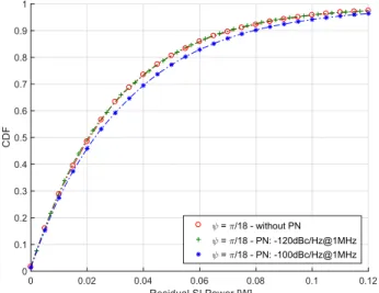
Next we analyze the impact of the oscillator’s phase-noise ( (t)) on the residual SI power. We consider a typical phase-noise value for a low power low area oscillator, built in a standard 130 nm CMOS technology, operating at 1 GHz [43], which may typically exhibit a phase-noise of approximately -100 dBc/Hz @ 1 MHz frequency offset. To determine the properties of the Gaussian distribution that represents the phase-noise, the oscillator phase-noise was simulated using the Matlab software package. The phase-noise distribution obtained from the data simulated with the phase-noise Simulink block was caracterized by a Gaussian distribution, N (µpn = 0, 2pn = 16⇥ 10 4). We have
also assumed RC oscillators, by considering the minimum achievable phase noise threshold, which is approximately -120 dBc/Hz [44]. For this case the oscillator phase-noise is also represented by a Gaussian distribution, N (µpn =
0, 2
pn = 16⇥ 10 6). We simulated the phase-noise with
a sample period T = Tc/360and (t) was added to the the
upconverted signal. Thus, instead of using (2) to compute the residual SI, we considered the phase noise and the residual SI was computed with the following formula
yrsi(t) = h xsi(t ⌧ )e
j(!c(t ⌧ )+ (t ⌧ ))
hcxsi(t ⌧c)ej(!c(t ⌧c)+ (t ⌧c)).
As can be seen in Fig. 6, the quality of the oscillators impacts
(a) CDF
(b) PDF
FIGURE 4: Residual SI Power for different values of KdB
(Rician fading: {KdB = -10 dB; µh = 0.3015; h = 0.6742},
{KdB = 0 dB; µh = 0.7071; h = 0.5000}, {KdB = 10 dB;
µh= 0.9535; h= 0.2132}).
on the distribution of the residual SI power. At the minimum achievable phase noise threshold (-120 dBc/Hz @ 1 MHz), the impact of the phase-noise on the distribution of the residual SI power is almost negligible. But, as the phase-noise increases (-100 dBc/Hz @ 1 MHz) the average of the residual SI power also increases.
V. CONCLUSIONS
A. APPLICABILITY OF THE PROPOSED APPROACH
It is well known that the knowledge of the residual SI due to the analog-domain cancellation is crucial to design efficient SI estimation methods to be used in the digital-domain. By doing so, the efficiency of the joint AC and DC schemes may be improved. The analytical derivation of the distribution of the residual SI power presented in this paper can be used to provide technical criteria for mitigating the SI residual
FIGURE 5:Residual SI Power for different sampling periods
of Xr+ jXj(Rician fading: KdB= 3 dB, µh= 0.8162, h=
0.4086; = ⇡/6).
interference in practical FDX communication systems. An obvious application is the compensation of the cancelation errors, which include the gain cancelation error (1 ✏) and the phase cancellation error ( ). By using the theoretical derivation presented in Section III and multiple samples of the residual SI collected in a practical FDX system, differ-ent estimation techniques can be employed to estimate the cancelation errors and compensate them (including but not limited to the method of moments3). However, the proposed
derivation can also be useful for the academic community in general, to determine different aspects related with the performance analysis of FDX communications, including for example the capacity of FDX communication systems by using the residual SI power to derive the outage probability
3In this case a channel estimation technique must also be employed to determine the channel statistics (hj, hr, h, µh,or #).
FIGURE 6:Residual SI Power for different values of
of a specific FDX system.
Finally, we highlight that although our work considers a single-tap delay channel, the approach may also be adopted in a multi-path scenario to provide an approximation of the residual SI. In FDX systems the LOS component is usually much higher than the non-LOS components (e.g. [42] reports 20-45 dBs higher). In this case, when the aggregated power of the non-LOS components is relatively low, our model can capture a significant amount of the residual SI power.
B. FINAL REMARKS
This work derives the distribution of the residual SI power due to channel estimation errors at the analog cancella-tion process. Closed form expressions were derived for the distribution of the residual self-interference power when Rician and Rayleigh fading self-interference channels are considered. Moreover, the distribution of the residual self-interference power was derived for low and high channel gain dynamics, by considering a invariant and a time-variant channel, respectively. The accuracy of the theoretical approach was assessed through Monte Carlo simulations for different levels of channel gain cancellation and phase errors during the channel estimation process. The results re-ported in the paper show that the channel dynamics strongly influence the distribution of the residual self-interference power. While for time-invariant channels the residual self-interference power is exponentially distributed, for time-variant channels the exponential distribution is not a valid assumption. Instead, the distribution of the residual self-interference power in time-variant channels can be approx-imated by a product distribution, as described in Theorem 1, which constitutes the main contribution of this work.
REFERENCES
[1] D. Kim, H. Lee, and D. Hong, “A Survey of In-Band Full-Duplex Trans-mission: From the Perspective of PHY and MAC Layers,” IEEE Commun. Surveys Tuts., vol. 17, no. 4, pp. 2017–2046, 4th Quart. 2015.
[2] M. Heino, D. Korpi, T. Huusari, E. Antonio-Rodriguez, S. Venkatasub-ramanian, T. Riihonen, L. Anttila, C. Icheln, K. Haneda, R. Wichman, and M. Valkama, “Recent advances in antenna design and interference cancellation algorithms for in-band full duplex relays,” IEEE Commun. Mag., vol. 53, no. 5, pp. 91–101, May 2015.
[3] Z. Zhang, X. Chai, K. Long, A. V. Vasilakos, and L. Hanzo, “Full duplex techniques for 5g networks: self-interference cancellation, protocol design, and relay selection,” IEEE Commun. Mag., vol. 53, no. 5, pp. 128–137, May 2015.
[4] J. I. Choi, M. Jain, K. Srinivasan, P. Levis, and S. Katti, “Achieving Single Channel, Full Duplex Wireless Communication,” in Proc. 16th Annu. Int. Conf. Mobile Comput. Netw., New York, NY, USA, 2010, pp. 1–12. [5] L. Wang, F. Tian, T. Svensson, D. Feng, M. Song, and S. Li, “Exploiting
full duplex for device-to-device communications in heterogeneous net-works,” IEEE Commun. Mag., vol. 53, no. 5, pp. 146–152, May 2015. [6] S. Goyal, P. Liu, S. S. Panwar, R. A. Difazio, R. Yang, and E. Bala,
“Full duplex cellular systems: will doubling interference prevent doubling capacity?” IEEE Commun. Mag., vol. 53, no. 5, pp. 121–127, May 2015. [7] D. Kim, S. Park, H. Ju, and D. Hong, “Transmission capacity of
full-duplex-based two-way ad hoc networks with arq protocol,” IEEE Trans. Veh. Technol., vol. 63, no. 7, pp. 3167–3183, Sep. 2014.
[8] X. Xie and X. Zhang, “Does full-duplex double the capacity of wireless networks?” in Proc. IEEE INFOCOM, Toronto, ON, Canada, Apr. 2014, pp. 253–261.
[9] E. Ahmed and A. M. Eltawil, “All-digital self-interference cancellation technique for full-duplex systems,” IEEE Trans. Wireless Commun., vol. 14, no. 7, pp. 3519–3532, Jul. 2015.
[10] D. Korpi, L. Anttila, V. Syrjala, and M. Valkama, “Widely Linear Digital Self-Interference Cancellation in Direct-Conversion Full-Duplex Transceiver,” IEEE J. Sel. Areas Commun., vol. 32, no. 9, pp. 1674–1687, Sep. 2014.
[11] D. Korpi, T. Riihonen, V. Syrjälä, L. Anttila, M. Valkama, and R. Wich-man, “Full-Duplex Transceiver System Calculations: Analysis of ADC and Linearity Challenges,” IEEE Trans. Wireless Commun., vol. 13, no. 7, pp. 3821–3836, July 2014.
[12] B. Debaillie, D. van den Broek, C. Lavín, B. van Liempd, E. A. M. Klumperink, C. Palacios, J. Craninckx, B. Nauta, and A. Pärssinen, “Analog/RF Solutions Enabling Compact Full-Duplex Radios,” IEEE J. Sel. Areas Commun., vol. 32, no. 9, pp. 1662–1673, Sep. 2014. [13] J. Lee, “Self-Interference Cancelation Using Phase Rotation in
Full-Duplex Wireless,” IEEE Trans. Veh. Technol., vol. 62, no. 9, pp. 4421– 4429, Nov. 2013.
[14] D. Bharadia and S. Katti, “Full Duplex MIMO Radios,” in Proc. 11th USENIX Symp. Netw. Syst. Design Implement., Seattle, WA, USA, Apr. 2014, pp. 359–372.
[15] L. Laughlin, M. Beach, K. Morris, and J. Haine, “Optimum Single An-tenna Full Duplex Using Hybrid Junctions,” IEEE J. Sel. Areas Commun., vol. 32, no. 9, pp. 1653–1661, Sep. 2014.
[16] E. Foroozanfard, O. Franek, A. Tatomirescu, E. Tsakalaki, E. de Carvalho, and G. Pedersen, “Full-duplex MIMO system based on antenna cancel-lation technique,” Electronics Lett., vol. 50, no. 16, pp. 1116–1117, Jul. 2014.
[17] P. Pursula, M. Kiviranta, and H. Seppa, “UHF RFID Reader With Re-flected Power Canceller,” IEEE Microw. Wireless Compon. Lett., vol. 19, no. 1, pp. 48–50, Jan. 2009.
[18] D. Bharadia, E. McMilin, and S. Katti, “Full Duplex Radios,” in Proc. ACM SIGCOMM Conf., Hong Kong, China, 2013, pp. 375–386. [19] R. Li, A. Masmoudi, and T. Le-Ngoc, “Self-Interference Cancellation With
Nonlinearity and Phase-Noise Suppression in Full-Duplex Systems,” IEEE Trans. Veh. Technol., vol. 67, no. 3, pp. 2118–2129, Mar. 2018. [20] A. Sahai, G. Patel, C. Dick, and A. Sabharwal, “Understanding the impact
of phase noise on active cancellation in wireless full-duplex,” in Proc. Asilomar Conf. Signals, Syst. Comput., Nov. 2012, pp. 29–33.
[21] M. Duarte, “Full-duplex Wireless: Design, Implementation and Character-ization,” Ph.D. dissertation, Houston, TX, USA, 2012.
[22] A. Masmoudi and T. Le-Ngoc, “A Maximum-Likelihood Channel Esti-mator for Self-Interference Cancelation in Full-Duplex Systems,” IEEE Trans. Veh. Technol., vol. 65, no. 7, pp. 5122–5132, Jul. 2016.
[23] A. Sahai, G. Patel, C. Dick, and A. Sabharwal, “On the Impact of Phase Noise on Active Cancelation in Wireless Full-Duplex,” IEEE Trans. Veh. Technol., vol. 62, no. 9, pp. 4494–4510, Nov. 2013.
[24] S. Li and R. Murch, “An Investigation Into Baseband Techniques for Single-Channel Full-Duplex Wireless Communication Systems,” IEEE Trans. Wireless Commun., vol. 13, no. 9, pp. 4794–4806, Sep. 2014. [25] M. Sakai, H. Lin, and K. Yamashita, “Adaptive cancellation of
self-interference in full-duplex wireless with transmitter IQ imbalance,” in Proc. IEEE GLOBECOM, Dec. 2014, pp. 3220–3224.
[26] E. Ahmed and A. Eltawil, “On Phase Noise Suppression in Full-Duplex Systems,” IEEE Trans. Wireless Commun., vol. 14, no. 3, pp. 1237–1251, Mar. 2015.
[27] V. Syrjala, M. Valkama, L. Anttila, T. Riihonen, and D. Korpi, “Analysis of Oscillator Phase-Noise Effects on Self-Interference Cancellation in Full-Duplex OFDM Radio Transceivers,” IEEE Trans. Wireless Commun., vol. 13, no. 6, pp. 2977–2990, Jun. 2014.
[28] M. Duarte, C. Dick, and A. Sabharwal, “Experiment-Driven Characteriza-tion of Full-Duplex Wireless Systems,” IEEE Trans. Wireless Commun., vol. 11, no. 12, pp. 4296–4307, Dec. 2012.
[29] Y.-S. Choi and H. Shirani-Mehr, “Simultaneous Transmission and Recep-tion: Algorithm, Design and System Level Performance,” IEEE Trans. Wireless Commun., vol. 12, no. 12, pp. 5992–6010, Dec. 2013. [30] M. Duarte, A. Sabharwal, V. Aggarwal, R. Jana, K. Ramakrishnan,
C. Rice, and N. Shankaranarayanan, “Design and Characterization of a Full-Duplex Multiantenna System for WiFi Networks,” IEEE Trans. Veh. Technol., vol. 63, no. 3, pp. 1160–1177, Mar. 2014.
[31] T. Riihonen, S. Werner, and R. Wichman, “Mitigation of Loopback Self-Interference in Full-Duplex MIMO Relays,” IEEE Trans. Signal Process., vol. 59, no. 12, pp. 5983–5993, Dec. 2011.
[32] B. Day, A. Margetts, D. Bliss, and P. Schniter, “Full-Duplex MIMO Relaying: Achievable Rates Under Limited Dynamic Range,” IEEE J. Sel. Areas Commun., vol. 30, no. 8, pp. 1541–1553, Sep. 2012.
[33] L. Irio, R. Oliveira, and L. Oliveira, “Characterization of the residual self-interference power in full-duplex wireless systems,” in Proc. IEEE Int. Symp. Circuits Syst., Florence, Italy, May 2018, pp. 1–5.
[34] A. Masmoudi and T. Le-Ngoc, “Self-interference cancellation limits in full-duplex communication systems,” in Proc. IEEE Global Telecomm. Conf., Washington, DC, USA, Dec. 2016, pp. 1–6.
[35] X. Li, C. Tepedelenlioglu, and H. Senol, “Channel Estimation for Residual Self-Interference in Full-Duplex Amplify-and-Forward Two-Way Relays,” IEEE Trans. Wireless Commun., vol. 16, no. 8, pp. 4970–4983, Aug. 2017. [36] A. Nadh, J. Samuel, A. Sharma, S. Aniruddhan, and R. K. Ganti, “A Taylor Series Approximation of Self-Interference Channel in Full-Duplex Radios,” IEEE Trans. Wireless Commun., vol. 16, no. 7, pp. 4304–4316, Jul. 2017.
[37] L. Samara, M. Mokhtar, Ö. Özdemir, R. Hamila, and T. Khattab, “Residual Self-Interference Analysis for Full-Duplex OFDM Transceivers Under Phase Noise and I/Q Imbalance,” IEEE Commun. Lett., vol. 21, no. 2, pp. 314–317, Feb. 2017.
[38] A. Shojaeifard, K. Wong, M. D. Renzo, G. Zheng, K. A. Hamdi, and J. Tang, “Self-Interference in Full-Duplex Multi-User MIMO Channels,” IEEE Commun. Lett., vol. 21, no. 4, pp. 841–844, Apr. 2017.
[39] L. Irio and R. Oliveira, “On the Impact of Fading on Residual Self-Interference Power of In-Band Full-Duplex Wireless Systems,” in Proc. Int. Wireless Commun. Mobile Comput. Conf. (IWCMC), Limassol, Cyprus, Jun. 2018, pp. 142–146.
[40] R. Navid, T. H. Lee, and R. W. Dutton, “Minimum achievable phase noise of rc oscillators,” IEEE Journal of Solid-State Circuits, vol. 40, no. 3, pp. 630–637, March 2005.
[41] D. Wulich, N. Dinur, and A. Glinowiecki, “Level clipped high-order OFDM,” IEEE Trans. Commun., vol. 48, no. 6, pp. 928–930, Jun. 2000. [42] E. Everett, A. Sahai, and A. Sabharwal, “Passive self-interference
suppres-sion for full-duplex infrastructure nodes,” IEEE Trans. Wireless Commun., vol. 13, no. 2, pp. 680–694, February 2014.
[43] S. Abdollahvand, J. Goes, L. B. Oliveira, L. Gomes, and N. Paulino, “Low phase-noise temperature compensated self-biased ring oscillator,” in Proc. IEEE Int. Symp. Circuits Syst., Seoul, South Korea, May 2012, pp. 2489– 2492.
[44] R. Navid, T. H. Lee, and R. W. Dutton, “Minimum achievable phase noise of rc oscillators,” IEEE J. Solid-State Circuits, vol. 40, no. 3, pp. 630–637, Mar. 2005.
LUIS IRIO received the M.Sc. degree in Electrical and Computer Engineering from Nova University of Lisbon in 2013. From 2014 to 2015, he was a Researcher at CTS-UNINOVA. He is currently an Ph.D. candidate in Electrical and Computer Engineering at Nova University of Lisbon and is also affiliated as a Researcher with Instituto de Telecomunicações. His research interests include Full-duplex systems, Multi-Packet Reception sys-tems and Wireless Mobile syssys-tems.
RODOLFO OLIVEIRA (S’04-M’10-SM’15) re-ceived the Licenciatura degree in electrical engi-neering from the Faculdade de Ciências e Tecnolo-gia (FCT), Universidade Nova de Lisboa (UNL), Lisbon, Portugal, in 2000, the M.Sc. degree in electrical and computer engineering from the In-stituto Superior Técnico, Technical University of Lisbon, in 2003, and the Ph.D. degree in electrical engineering from UNL, in 2009. From 2007 to 2008, he was a Visiting Researcher at the Uni-versity of Thessaly. From 2011 to 2012, he was a Visiting Scholar at the Carnegie Mellon University. Rodolfo Oliveira is currently with the Department of Electrical and Computer Engineering, UNL, and is also affiliated as a Senior Researcher with the Instituto de Telecomunicações, where he researches in the areas of Wireless Communications, Computer Networks, and Computer Science. He serves in the Editorial Board of Ad Hoc Networks (Elsevier).