Family Houses Energy Consumption Forecast Tools for
Smart Grid Management
F. Rodrigues1,2, C. Cardeira1, J.M.F. Calado1,3, R. Melício1,4 1IDMEC,Instituto Superior Técnico, Universidade de Lisboa, Lisbon, Portugal
2MIT Portugal, Porto Salvo, Portugal
3Departamento de Engenharia Mecânica,Instituto Superior de Engenharia de Lisboa, Portugal 4Departamento de Física,Escola de Ciências e Tecnologia, Universidade de Évora
Abstract. This paper presents a short term (ST) load forecast (FC) using Artificial
Neural Networks (ANNs) or Generalized Reduced Gradient (GRG). Despite the apparent natural unforeseeable behavior of humans, electricity consumption (EC) of a family home can be forecast with some accuracy, similarly to what the electric utilities can do to an agglomerate of family houses. In an existing electric grid, it is important to understand and forecast family house daily or hourly EC with a reliable model for EC and load profile (PF). Demand side management (DSM) programs required this information to adequate the PF of energy load diagram to Electric Generation (EG). In the ST, for load FC model, ANNs were used, taking data from a EC records database. The results show that ANNs or GRG provide a reliable model for FC family house EC and load PF. The use of smart devices such as Cyber-Physical Systems (CPS) for monitoring, gathering and computing a database, improves the FC quality for the next hours, which is a strong tool for Demand Response (DR) and DSM.
Keywords: Energy forecasting, energy management, smart grids, artificial neural
networks, gradient methods.
1 Introduction
The major objective of DSM is to encourage customer to participate in schemes to reduce peak demand and shifting the load. One such mechanism is DR, in which the system allows end users to alter their load shape to reduce the overall peak of the system [1]. An important tactic to DR and energy management to promote a more efficient energy end user is DSM [2]. DSM is based on a set of tools for shaping the load diagram, through peak clipping, valley filling, and shift of some loads, among others [3]. These strategies are required to conveniently shape the load EC diagram. In a Smart Grid (SGr) context, a consumer active role is essential for grid management in order to efficiently assure EG and usage.
Using the knowledge about the PF curve of power EC of each family house, a model for optimizing the electrical energy can be generated [4]. Tools for providing an accurate ST Load FC (STLFC) will enhance the quality of the DSM.
The aim of this paper is to show the use of an ANN and GRG to develop a simple and reliable method for STLFC of family houses’ daily and hourly EC for residential and small buildings.
ANNs are weel known by their ability of self learning and provide accurate predictions for many applications. Models achieved using ANN are inspired on the
human neurons behavior. Simple ‘neuron’ computations are performed locally and the connections among are adapted for defining the model. In [5] ANNs are used for predicting room temperatures. For this work, it was used a set of EC data from different family houses to train the ANN. The database used in this work comes from a study performed on 93 family houses, in Portugal [6].
The paper organization is as follows: Section 2 presents the state of the art. Section 3 presents the methodologies used in the paper: ANN and GRG. Section 4 presents case studies and results. Finally, conclusions are drawn in Section 5.
2 State of the Art
A large number of scientific works have been carried out about techniques for STLFC. Some techniques are very successful for power systems, while they underperform on other occasions due to the specific features of the local EC load: Models are difficult, are not linear and are subject to specific conditions like weather or social unexpected impacts.
Some scientific surveys were dedicated to ANNs for STLFC [7,9–14]. Other techniques were used such as time series and regression models [15,16]. In [17] a general overview of FC techniques is presented. ANNs have received a large share of attention and interest.
There is a direct connection of this work to SGrs and CPS. Renewable technologies highly present large production variation in function of the local weather. Their highly unpredictive nature increases the difficulty regarding their incorporation into the electric power distribution. This issue needs to be fully solved in SGr systems scope [7,8].
Sustainability is a major challenge for SGr [9]. Currently power systems are largely distributed and demand precise control. The need of an adequate response to severe faults is even more important, due to the generalization of the electrical markets. Power system currently based on SCADA systems are expected to evolved into SCADA systems, integrated in SGr systems. SCADA systems are usually pointed out as an reference example of CPS [10], intended to achieve a blackout-free EG and distribution system, for building SGrs, or for optimization of EC [9].
CPS can be described as smart systems including software and hardware, namely components for sensing, monitoring, gathering, actuating, computing, communication and controlling physical infrastructures, completely integrated and directly interacting to sense the alterations in the state of the surrounding environment [11].
The integration of renewable energy resources and electro-mobility into an electric grid, raises many concerns regarding operation, balance and reliability. Thus, the use of smart devices such as CPS, to assist monitoring, control and operating renewable energy systems in a SGr context [12,18] are fundamental pieces in the success of these systems. Also, in an existing electric grid, it is important to understand and FC family house daily or hourly EC with a reliable model for EC and load PF. The effectiveness of the DSM and DR programs highly depend on the quality of energy FC. DSM and DR programs require to adequate the PF of energy load diagram to EG. In STLFC model ANN have been used with an EC records database. However, using smart devices such as CPS monitoring, gathering and computing in real time a database with weekdays and weekend, the use of two groups of days, allow developing STLFC models with better results than a model that used a single week [13].
3 Methodologies
3.1 ANN
The network architecture that was built for FC is a feed-forward type of ANN. The backpropagation learning algorithm was used to train the ANN. Backpropagation learning algorithms are based on steepest descent methods. Looking to the output neurons results error, connections are updated to make the ANN closer to the model. As learning phase goes on the error is minimized.
The Levenberg-Marquardt Algorithm (LMA) consists in finding the update given by:
e(c)
(c)
J
I]
+
J(c)
(c)
-[J
=
c
T
-1 T
(1) where: J(c) is the Jacobian; µ is a adjustable factor; and e(c) is the error.A small µ is turns the LMA into a classic Gauss-Newton algorithm. Higher µ values turn the LMA into a steepest descent algorithm. The LMA, parametrized by µ may take advantage on the Gauss-Newton algorithm faster convergence or on the Steepest descent convergence guarantee [19].
Furthermore, the output of any neuron is shown in Fig. 1.
f(u
k)
uk yk Output Wk0 Wk1 Wk2 Wkm x0=+1 x1 x2 xm N eu ro n s in p u ts Bias input Neuron transfer function Connection weightsFig. 1. Neuron model
The neuron output value is given by:
)
(
)
(
1
m j k j kj k kf
u
f
W
x
b
y
. (2))
(
)
(
0
m j j kj k kf
u
f
W
x
y
(3)The number of inputs determines the number of input neurons. Accordingly, the number of variables to estimate determines the number of output neurons. The number of hidden neuros depends on the model.
Transfer functions of the neurons have to be differentiable and with a positive (or null) derivate [13]: Sigmoid functions are relatively common. Moreover, these functions scale the inputs to a continuous value between 0 a 1.
The ANN architecture was built with three-layer feedforward configuration. The network was optimized as mentioned in [4].
Fig. 2 shows the network used for predicting the hourly EC for an usual day. ANN inputs are the hourly EC of each family house.
Fig. 2. Simplified ANN Architecture used to FC hourly load.
For each family house around 500 hours of logged EC were available. 66% of this data was used for training, 2/3 of those data were used for ANN training and validation. 33% of those data were used to evaluate the FC quality.
Binary inputs were used to code the previous hours [20] for the hourly load FC [21]. The 11 input neurons are distributed as follows. Five correspond to the last five previous hours EC. The 6th input neuron corresponds to the EC during the last 24th hour. Five neurons are used to binary encode the hours. The hidden layer is composed by twenty neurons. The output is the next hour EC prediction.
3.2 GRG
GRG is another popular technique. The original method, the Reduced Gradient Method has seen several different customizations due several researchers [22,23]. The GRG formulation is given by the maximization of the following function:
U
c
L
c
g
c
f
(
k)
:
(
k)
0
,
min
(4)Where f(ck) is the objective function, subject to g(ck) function, where ck values are
constrained to the [L,U] interval.
4 Case Studies
Two case studies were performed to validate the models based on information from monitoring carried out in [4]. The algorithms were implemented in tool Matlab environment.
4.1 Case 1
Using Fig 2 model, the ANN two weeks of hourly EC were used for learning and the third week was used for testing the model. Results are shown in Fig. 3 a) and Fig. 3 b).
a) b)
Fig. 3. FC Hourly load of two random family houses.
Table 1 summarizes the results obtained for the linear correlation R and linear regression R2, mean absolute percent error (MAPE) and the standard deviation of error (SDE),.
Table 1. ANN FC results
Family house nº 64 Family house nº 65
R R2 MAPE SDE R R2 MAPE SDE
Day 1 99% 98% 16% 0,2 98% 97% 22% 0,2 Day 2 99% 99% 10% 0,1 98% 95% 19% 0,2 Day 3 99% 99% 13% 0,1 98% 93% 24% 0,2 Day 4 87% 75% 37% 0,7 96% 92% 23% 0,2 Day 5 72% 52% 61% 0,5 90% 68% 44% 0,5 Day 6 43% 18% 87% 0,8 86% 71% 45% 0,4 Day 7 93% 87% 30% 0,4 93% 89% 37% 0,2
As the family house EC load may be zero or change orders of magnitude along the day, the average load was used in MAPE to avoid the problem caused by zero loads. In linear correlation (R) and regression (R2) show how accurately the estimates compare to the real data.
Fig. 3 and Table 1 show that method proposed shows a decent FC performance. 4.2 Case 2
To optimize the solution and identify the type of function (linear or nonlinear) it was used the GRG method used by Solver. The results showed the functions of daily EC are nonlinear and the optimization tool can be used to FC annual EC average.
Using GRG, the research has shown the ability to converge the FC function to the function of real EC with an error MSE 0.
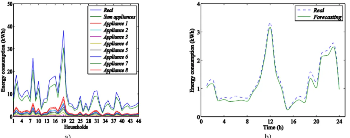
The comparison of an average annual daily EC with accumulative EC electric appliance FC is shown in Fig. 4 a).
The modeling tested results of Portuguese family house average annual daily EC is shown in Fig. 4 a). The horizontal axis identifies the family house number. The vertical axis shows the average annual daily EC in kWh per day. The straight blue line (from de top, first one) represents the total real average annual daily EC. The green line (second) represents accumulated average annual EC from appliances FC. Other colors represent the monitored electric appliance FC consumptions.
The comparison of hourly EC average using electric appliance FC is shown in Fig. 4 b). Fig. 4 b) shows the modeling tested results of family house hourly EC average. The blue line represents the hourly EC average and the green line represents the EC weights and the contribution of each appliance in a family house.
a) b)
Fig. 4. Average annual EC FC: a) appliance samples; b) random house.
The results show also the real load PF is always above the FC. One reason for this fact is that FC did not include all electric appliances (e.g: microwave, coffee machine, vacuum machine). The used database included total energy family house EC and EC of some specific electric appliance (washer, fridge, TV). The partial measures do not add-up total EC, because some other ECs were not measured and introduced in database. Therefore, is not surprising the estimated energy load PF is bellower than total EC.
However, Fig. 4 shows the FC follows the shape of the real load PF with a relative low offset. One explanation is that some ECs might exist besides the monitored electric appliances.
6 Conclusion
This paper present ANN and GRG methods for estimation of hourly EC. The FC models provided estimates of hourly EC and load PF with significant accuracy. The results show that ANNs performed well forecasting the load for the next days and GRG also exhibit good performance for the annual average EC.
FC hourly and daily EC are useful for DSM to fit the energy production to the expected consumption. Moreover, the knowledge about future consumption, it becomes possible to do shedding (anticipate or postpone) of the EC.
Future researches will be in towards the integration of these techniques in to smart devices such as CPS, to assist monitoring, control and operation of SGrs.
Acknowledgments
The authors thank for the Portuguese Funds support, through the FCT, project LAETA2015/2020, ref.UID/EMS/50022/2013.
References
1. Reka, S. Sofana, Ramesh, V.: A demand response modeling for residential consumers in smart grid environment using game theory based energy scheduling algorithm. Ain Shams Engineering Journal (2016)
2. Rodrigues, F., Cardeira, C., Calado, J.M.F., Melício, R.: Energy household forecast with ANN for demand response and demand side management. Renewable Energy and Power Quality Journal-ICREPQ 14:1–4 (2016)
3. Macedo, M.N.Q., Galo, J.J.M., de Almeida, L.A.L., de C. Lima, A.C.: Demand side management using artificial neural networks in a smart grid environment. Renewable and Sustainable Energy Reviews 41:128–133 (2015)
4. Rodrigues, F., Cardeira, C., Calado, J.M.F.: The daily and hourly energy consumption and load forecasting using artificial neural network method: a case study using a set of 93 households in Portugal. Energy Procedia 62:220–229 (2014)
5. Yang IH, Kim KW.: Prediction of the time of room air temperature descending for heating systems in buildings. Building and Environment 39(1):19–29 (2004)
6. Sidler, O.: Demand side management. End-use metering campaign in 400 households of the European Community. SAVE Programme, Project EURECO. Commission of the European Communities: France (2002)
7. Blaabjerg, F., Ionel, M.: Renewable energy devices and systems–state-of-the-art technology, research and development, challenges and future trends. Electric Power Components and Systems 43(12):1319–1328 (2015)
8. Viegas, J.L., Vieira, S.M., Melicio, R., Mendes, V.M.F., Sousa, J.M.C.: Classification of new electricity customers based on surveys and smart metering data. Energy 107: 804–817 (2016)
9. Ramos, C., Vale, Z., Faria, L.: Cyber-physical intelligence in the context of power systems. In Future Generation Information Technology 7105:19–29 (2011)
10. Faria, L., Silva, A., Ramos, C., Vale, Z., Marques, A.: Intelligent behavior in a cyber-ambient training system for control center operators. Proceedings of ISAP:1–6 (2011) 11. Ying, S.: Foundations for innovation in cyber-physical systems. Workshop Report,
Energetics Incorporated, Columbia, Maryland, US (2013)
12. Seixas, M., Melício, R., Mendes, V.M.F.: Simulation of rectifier voltage malfunction on OWECS, four-level converter, HVDC light link: smart grid context tool. Energy Conversion and Management 97:140–153 (2015)
13. Hippert, H., Pedreira, C., Souza, R.: Neural networks for short-term load forecasting: a review and evaluation. IEEE Transactions on Power Systems 16(1):44–55 (2001) 14. Carpinteiro, O., Reis, A., Silva, A.: A hierarchical neural model in short-term load
15. Gross, G., Galiana, F.: Short-term load forecasting. Proceedings of IEEE 75(12): 1558–1573 (1987)
16. Taylor, J.: Short-term load forecasting with exponentially weighted methods. Power Systems, IEEE Transactions on 27(1):458–464 (2012)
17. Feinberg, E., Genethliou, D.: Load forecasting. Applied mathematics for restructured electric power systems. Springer US:269–285 (2005)
18. Viegas, J.L., Vieira, S.M., Melicio, R., Mendes, V.M.F., Sousa, J.M.C.: GA-ANN short-term electricity load forecasting. In: Technological Innovation for Cyber-Physical Systems, Eds. L.M. Camarinha-Matos, António J. Falcão, Nazanin Vafaei, Shirin Najdi, 7th IFIP AICT 470, Springer:485–493 (2016)
19. Saini, L., Soni, M.: Artificial neural network based peak load forecasting using Levenberg-Marquardt and quasi-Newton methods. IEE Proceedings-Generation, Transmission and Distribution 149(5): 578–584 (2002)
20. Holderbaum, W., Canart, R., Borne, P.: Artificial neural networks application to boolean input systems control. Studies in Informatics and Control 8:107–120 (1999) 21. Zebulum, R.S., Vellasco, M., Guedes, K., Pacheco, M.A.: Short-term load forecasting
using neural nets. In Natural to Artificial Neural Computation 1001–1008 (1995) 22. Luenberger, D.G., Ye, Y.:Linear and nonlinear programming. Springer, Stanford, USA
(2008)
23. Lasdon, L.S., Waren, A.D., Jain, A., Ratner, M.: Design and testing of a generalized reduced gradient code for nonlinear programming.ACM Transactions on Mathematical Software 4(1): 34–50 (1978)