A SOM-based hierarchical model to short-term load
forecasting
Ot´avio A. S. Carpinteiro, Agnaldo J. R. Reis
Research Group on Computer Networks and Software Engineering Federal University of Itajub´a
37500–903, Itajub´a, MG, Brazil E-mails:{otavio,agnreis}@iee.efei.br
Abstract— This paper proposes a SOM-based hierarchical neural model to the problem of short-term load forecasting. The neural model is made up of two self-organizing map nets — one on top of the other. It has been successfully applied to domains which require time series analysis. The model was trained and assessed on load data extracted from a Brazilian electric utility. It was required to predict once every hour the electric load during the next 24 hours. The paper presents the results, and evaluates them.
I. INTRODUCTION
Short-term forecasting of load demand is necessary for the correct operation of electric utilities. Forecasts are required for proper scheduling activities, such as generation scheduling, fuel purchasing scheduling, maintenance scheduling, and for security analysis [1].
Conventional load forecasting techniques, based on statisti-cal methods, fail to provide accurate results. Moreover, they hold several weaknesses, including complexity of modelling, and lack of flexibility [2].
Neural networks (NNs) have succeeded in several power system problems, such as planning, control, analysis, protec-tion, design, load forecasting, security analysis, and fault diag-nosis. The last three are the most popular [3]. The NN ability in mapping complex non-linear relationships is responsible for the growing number of its application to the short-term load forecasting (STLF) [4], [5], [6], [2].
So far, the great majority of proposals on the application of NNs to STLF use the multilayer perceptron (MLP) trained with error backpropagation. Besides the high computational burden for supervised training, MLPs do not have a good ability to detect data outside the domain of the training data. This paper introduces a hierarchical neural model (HNM) to STLF. The HNM is based on the Kohonen’s original self-organizing map (SOM) [7]. The hierarchical topology yields to the model the power to process efficiently the context information embedded in the historical load series. The model does not suffer from loss of context [8]. On the contrary, it holds a very good memory for past events, enabling it to produce better forecasts. It has been applied to load data extracted from a Brazilian electric utility.
This paper is divided as follows. The second section provides an overview of related research. The third section presents the data representation. The HNM is introduced in
the fourth section. The fifth section describes the experiments, and discusses the results. The last section presents the main conclusions of the paper, and indicates some directions for future work.
II. RELATED RESEARCH
The importance of short-term load forecasting has been increasing lately. With deregulation and competition, energy price forecasting has become a valuable business. Bus-load forecasting is essential to feed analytical methods utilized for determining energy prices. The variability and non-stationarity of loads are becoming critical owing to the dynamics of energy prices. In addition, the number of nodal loads to be predicted does not allow frequent interactions with load forecasting experts. More autonomous load predictors are needed in the new competitive scenario.
Artificial neural networks (NNs) have been successfully applied to short-term load forecasting (STLF). Many electric utilities, which had previously employed STLF tools based on classical statistical techniques, are now using NN-based STLF tools.
Park et al. [9] have successfully introduced an approach to STLF which employs a NN as main part of the forecaster. The authors employed a feed-forward neural network trained with the standard error backpropagation algorithm (EBP). Three NN-based predictors have been developed and applied to short-term forecasting of daily peak load, total daily energy, and hourly daily load, respectively. Three months of actual load data from Puget Sound Power and Light Company have been used in order to test the aforementioned forecasters. Only ordinary weekdays were taken into consideration for the training data.
Another successful example of NN-based STLF can be found in Lee et al. [10]. The authors employed a multilayer perceptron (MLP) trained with EBP to predict the hourly load for a lead time of 1–24 hours. Two different approaches have been considered, namely one-step ahead forecasting (named static approach), and 1–24 steps ahead (named dynamic ap-proach). In both cases, the load was separated in weekday (Tuesdays through Fridays) and weekend loads (Saturdays through Mondays).
for the Greek power system. The authors made use of the previous year for training purposes. Holidays were excluded from the training set and treated separately. The network was retrained daily using a moving window of the 365 most recent input/output patterns. More, the paper proposed another procedure to 2–7 days ahead forecasting.
Papalexopoulos et al. [11] compared the performance of a sophisticated regression-based forecasting model to a newly developed NN-based model for STLF. It is worth mentioning that the regression model had been in operation in a North-American utility for several years, and represented the state-of-art in the classical statistical approach to STLF. The NN-based model has outperformed the regression model, yielding better forecasts. Moreover, the development time of the neural model was shorter, and the development costs lower in comparison to the regression model. As a consequence, the neural model has replaced the regression model. This report is important, for it evaluates the operation of a neural model in a realistic electrical utility environment.
Khotanzad et al. [5] describe the third generation of an hourly short-term load forecasting system, named artificial neural network short-term load forecaster (ANNSTLF). Its architecture includes only two neural forecasters — one fore-casts the base load, and the other predicts the change in load. The final prediction is obtained via adaptive combination of these two forecasts. A novel scheme for forecasting holiday loads is developed as well. The performance on data from ten different utilities is reported and compared to the previous generation forecasting system.
Finally, a comprehensive review of the application of NNs to STLF can be found in Hippert et al. [6]. The authors examine a collection of papers published between 1991 and 1999.
III. DATA REPRESENTATION
The input data consisted of sequences of load data extracted from a Brazilian electric utility. Weather data were not in-cluded, for they were not available.
Seven neural input units are used in the representation, as shown in table I. The first unit represents the load at the current hour. The second, the load at the hour immediately before. The third, fourth and fifth units represent respectively the load at twenty-four hours behind, at one week behind, and at one week and twenty-four hours behind the hour whose load is to be pre-dicted. The sixth and seventh units represent a trigonometric coding for the hour to be forecast, i.e., sin(2π.hour/24)and cos(2π.hour/24). Each unit receives real values. The load data is preprocessed using ordinary normalization (minimum and maximum values in the [0,1] range).
IV. THEHNM
The model is made up of two self-organizing maps (SOMs), as shown in figure 1. Its features, performance, and potential are better evaluated in [8], [12].
The input to the model is a sequence in time of m -dimensional vectors,S1=V(1),V(2), . . . ,V(t), . . . ,V(z),
where the components of each vector are real values. The
V(t)
SOM Bottom SOM Top
Time Integrator
Map Map
Time Integrator
Λ
Fig. 1. HNM
sequence is presented to the input layer of the bottom SOM, one vector at a time. The input layer hasmunits, one for each component of the input vectorV(t), and a time integrator. The
activationX(t) of the units in the input layer is given by X(t) =V(t) +δ1X(t−1) (1)
where δ1 ∈ (0,1) is the decay rate. For each input vector
X(t), the winning uniti∗(t)in the map is the unit which has
the smallest distance Ψ(i, t). For each output uniti, Ψ(i, t)
is given by the Euclidean distance between the input vector
X(t)and the unit’s weight vectorWi.
Each output unit i in the neighbourhood N∗(t) of the
winning uniti∗(t)has its weightWi updated by
Wi(t+ 1) =Wi(t) +αΥ(i)[X(t)−Wi(t)] (2) whereα∈(0,1) is the learning rate.Υ(i) is the neighbour-hood interaction function[13], a Gaussian type function, and is given by
Υ(i) =κ1+κ2e−
κ3[Φ(i,i∗(t))]2
2σ2 (3)
where κ1, κ2, and κ3 are constants, σ is the radius of the neighbourhood N∗(t), and Φ(i, i∗(t)) is the distance in the
map between the unit i and the winning unit i∗(t). The
distanceΦ(i′, i′′)between any two unitsi′ andi′′in the map
is calculated according to the maximum norm,
Φ(i′, i′′) =max{|l′−l′′|,|c′−c′′|} (4)
where (l′, c′) and(l′′, c′′) are the coordinates of the units i′
andi′′ respectively in the map.
The input to the top SOM is determined by the distances
Φ(i, i∗(t))of thenunits in the map of the bottom SOM. The
input is thus a sequence in time ofn-dimensional vectors,S2
= Λ(Φ(i, i∗(1))), Λ(Φ(i, i∗( 2))), . . . , Λ(Φ(i, i∗(t))), . . . , Λ(Φ(i, i∗(z))), where Λ is an-dimensional transfer function
TABLE I
INP UT VARI ABLES F OR THEHNMM ODEL
Input Variable name Lagged values (h)
1–5 Load(P) 1, 2, 24, 168, 192
6 HS 0∗
7 HC 0∗
∗Lag 0 represents the hour to be forecast
Λ(Φ(i, i∗( t))) =
1−κΦ(i, i∗(t)) ifi∈N∗(t) 0 otherwise (5)
where κis a constant, and N∗(t) is a neighbourhood of the
winning unit.
The sequenceS2 is then presented to the input layer of the
top SOM, one vector at a time. The input layer has n units, one for each component of the input vectorΛ(Φ(i, i∗(t))), and
a time integrator. The activationX(t)of the units in the input
layer is thus given by
X(t) = Λ(Φ(i, i∗(t))) +δ
2X(t−1) (6)
whereδ2∈(0,1)is the decay rate.
The dynamics of the top SOM is identical to that of the bottom SOM.
V. EXPERIMENTS
Two different hierarchical neural models are conceived. The first one is required to foresee the time horizon from the first to the sixth hour. The training of the two SOMs of this model takes place in two phases — coarse-mapping and fine-tuning. In the coarse-mapping phase, the learning rate and the radius of the neighbourhood are reduced linearly whereas in the fine-tuning phase, they are kept constant. The bottom and top SOMs were trained respectively with map sizes of 15×15 in 700 epochs, and 18×18 in 850 epochs. It was used low values for decay rates — 0.4 and 0.7 for the bottom and top SOMs, respectively. According to Carpinteiro [8], low decay rates reduce the memory size for past events. By using low decay rates, it is thus reduced the memory for the former day predictions. The initial weights were given randomly to both SOMs.
The forecasting of the remaining time — seventh to twenty-fourth hour — is addressed by the second model. The same training process previously described is applied to this model too. Nevertheless, medium values for decay rates — 0.5 and 0.8 for the bottom and top SOMs, respectively — were used instead. These new values for decay rates extend the memory size for past events [8], and consequently, yield more accurate predictions on large horizons.
The training set comprised 2160 load patterns, spanning ninety days. The maximum electric load fell around 3900 MWatts. There was no particular treatment for holidays.
The inclusion of temperatures in the training set is still an open question. Many researchers have included them, although the benefits which neural models may reap from those vari-ables in daily forecasting be controversial [2]. Weather data were not included in the training set anyway, for they were not available on those ninety days at the region in which the utility operated.
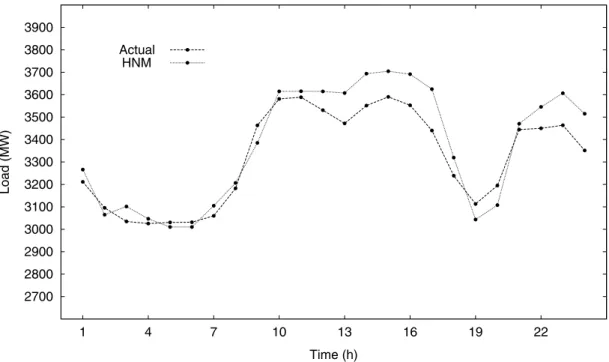
Figures 2 and 3 show the actual load and forecast load for two particular days. The first one — Friday, February 03, 1995 — is a typical weekday, and the second one — Tuesday, February 07, 1995 — is a special weekday.
A typical weekday is one whose load patterns share some similarity with the load patterns of the same weekdays in former weeks. For instance, the load patterns for Tuesdays tend to display a similar behaviour. Yet, when an unexpected event, such as a holliday, happens on one of those Tuesdays, it changes that fairly stationary behaviour. Such holliday is then said to be a special weekday. Special weekdays break down forecasters, for they perform much better on typical than on special weekdays.
Table II presents the performance of the forecasters for one to twenty-four step ahead predictions on those weekdays, as well as the mean absolute percentage error (MAPE).
The results from the HNM are very promising. They were compared to the results from a multilayer perceptron (MLP), working on the same 2160 load patterns [14]. According to such results, MLP obtained MAPE values of 2.64 and 5.92 for the typical and special weekdays respectively.
2700 2800 2900 3000 3100 3200 3300 3400 3500 3600 3700 3800 3900
1 4 7 10 13 16 19 22
Load (MW)
Time (h) Actual
HNM
Fig. 2. Actual load and forecast load for February 03, 1995
2600 2700 2800 2900 3000 3100 3200 3300 3400 3500 3600 3700 3800
1 4 7 10 13 16 19 22
Load (MW)
Time (h) Actual
HNM
TABLE II
HOURLY P ERCENTAGE ERROR F ORFEBRUARY03AND07, 1995
Time (h) Feb. 03 Feb. 07
1 1.70 0.11
2 0.99 1.14
3 2.19 0.41
4 0.70 0.58
5 0.68 0.12
6 0.71 1.04
7 1.47 2.98
8 0.76 0.43
9 2.26 1.31
10 0.94 1.75
11 0.74 1.90
12 2.37 1.02
13 3.90 1.04
14 4.01 3.54
15 3.19 0.90
16 3.89 0.63
17 5.36 1.86
18 2.49 6.11
19 2.24 1.85
20 2.74 1.81
21 0.75 2.19
22 2.77 1.24
23 4.12 6.38
24 4.89 8.30
MAPE (%) 2.33 2.03
VI. CONCLUSION
The paper presents a novel artificial neural model for se-quence classification and prediction. The model has a topology made up of two self-organizing map networks, one on top of the other. It encodes and manipulates context information effectively.
The results obtained have shown that the HNM was able to perform efficiently the prediction of the electric load in both very short and short forecasting horizons. Furthermore, the results are better than those obtained by MLP on equal data.
It is worth mentioning that MLP has been widely employed to tackle the problem of STLF so far. The results obtained thus suggest that HNM may offer a better alternative to approach such problem.
A research and development project for a Brazilian electric utility is under course. The research will focus on the effects of the HNM time integrators on the predictions in order to produce a better adaptability. Besides, it will focus on the study of its performance on larger databases which include both
load and weather data. The forecasts should also span a larger number of days in order to be more significant statistically.
ACKNOWLEDGMENT
This research is supported by CNPq, Brazil.
REFERENCES
[1] D. Ranaweera, G. Karady, and R. Farmer, “Economic impact analysis of load forecasting,”IEEE Trans. on Power Systems, vol. 12, no. 3, pp. 1388–1392, Aug 1997.
[2] F. Marin, F. Garcia-Lagos, G. Joya, and F. Sandoval, “Global model for short-term load forecasting using artificial neural networks,”IEE Proc. Gener. Transm. Distrib., vol. 149, no. 2, pp. 121–125, Mar 2002. [3] H. Mori, “State-of-the-art overview on artificial neural networks in
power systems,” in A Tutorial Course on Artificial Neural Networks with Applications to Power Systems, M. El-Sharkawi and D. Niebur, Eds. IEEE Power Engineering Society, 1996, ch. 6, pp. 51–70. [4] A. Bakirtzis, V. Petridis, S. Klartzis, M. Alexiadis, and A. Maissis, “A
[5] A. Khotanzad, R. Afkhami-Rohani, and D. Maratukulam, “ANNSTLF – artificial neural network short-term load forecaster – generation three,” IEEE Trans. on Power Systems, vol. 13, no. 4, pp. 1413–1422, Nov 1998.
[6] H. Hippert, C. Pedreira, and R. Souza, “Neural networks for short-term load forecasting: A review and evaluation,”IEEE Trans. on Power Systems, vol. 16, no. 1, pp. 44–55, Feb 2001.
[7] T. Kohonen, Self-Organizing Maps, 3rd ed. Berlin: Springer-Verlag, 2001.
[8] O. A. S. Carpinteiro, “A hierarchical self-organizing map model for pattern recognition,” in Proceedings of the Brazilian Congress on Artificial Neural Networks 97 (CBRN 97), L. Caloba and J. Barreto, Eds., Florian´opolis, SC, Brazil, 1997, pp. 484–488.
[9] D. Park, M. El-Sharkawi, R. Marks II, L. Atlas, and M. Damborg, “Electric load forecasting using an artificial neural network,” IEEE Trans. on Power Systems, vol. 6, no. 2, pp. 442–449, May 1991.
[10] K. Lee, Y. Cha, and J. Park, “Short-term load forecasting using an artificial neural network,”IEEE Trans. on Power Systems, vol. 7, no. 1, pp. 124–132, Feb 1992.
[11] A. Papalexopoulos, S. Hao, and T. Peng, “An implementation of a neural network based load forecasting model for the EMS,”IEEE Trans. on Power Systems, vol. 9, no. 4, pp. 1956–1962, Nov 1994.
[12] O. A. S. Carpinteiro, “A hierarchical self-organizing map model for se-quence recognition,” inProceedings of the International Conference on Artificial Neural Networks 98, L. Niklasson, M. Bod´en, and T. Ziemke, Eds., Sk¨ovde, Sweden, 1998, pp. 815–820.
[13] Z. Lo and B. Bavarian, “Improved rate of convergence in Kohonen neural network,” in Proceedings of the International Joint Conference on Neural Networks, vol. 2, July 8–12 1991, pp. 201–206.