A HIERARCHICAL SELF-ORGANIZING MAP MODEL IN SHORT-TERM LOAD FORECASTING
Ot´avio A. S. Carpinteiro, Agnaldo J. R. Reis∗
∗ Research Group on Computer Networks and Software Engineering
Federal University of Itajub´a 37500–903, Itajub´a, MG, Brasil
Email: {otavio,agnreis}@iee.efei.br
Abstract— This paper proposes a novel neural model to the problem of short-term load forecasting. The neural model is made up of two self-organizing map nets — one on top of the other. It has been successfully applied to domains in which the context information given by former events plays a primary role. The model was trained and assessed on load data extracted from a Brazilian electric utility. It was required to predict once every hour the electric load during the next 24 hours. The paper presents the results, and evaluates them.
Keywords— short-term load forecasting; self-organizing map; neural network.
1 Introduction
With power systems growth and the increase in their complexity, many factors have become in-fluential to the electric power generation and consumption (e.g., load management, energy ex-change, spot pricing, independent power produc-ers, non-conventional energy, generation units, etc.). Therefore, the forecasting process has be-come even more complex, and more accurate forecasts are needed. The relationship between the load and its exogenous factors is complex and non-linear, making it quite difficult to model through conventional techniques, such as time se-ries and linear regression analysis. Besides not giving the required precision, most of the tradi-tional techniques are not robust enough. They fail to give accurate forecasts when quick weather changes occur. Other problems include noise im-munity, portability and maintenance (Khotanzad et al., 1995).
Neural networks (NNs) have succeeded in sev-eral power system problems, such as planning, control, analysis, protection, design, load forecast-ing, security analysis, and fault diagnosis. The last three are the most popular (Mori, 1996). The NN ability in mapping complex non-linear rela-tionships is responsible for the growing number of its application to the short-term load forecasting (STLF) (Liu et al., 1996; Bakirtzis et al., 1996; Mohammed et al., 1995; Park et al., 1991). Sev-eral electric utilities over the world have been ap-plying NNs for load forecasting in an experimental or operational basis (Khotanzad et al., 1995; Mori, 1996; Bakirtzis et al., 1996).
So far, the great majority of proposals on the application of NNs to STLF use the multilayer perceptron (MLP) trained with error backpropa-gation. Besides the high computational burden for supervised training, MLPs do not have a good ability to detect data outside the domain of the training data.
This paper introduces a new hierarchical neu-ral model (HNM) to STLF. The HNM is an exten-sion of the Kohonen’s original self-organizing map (Kohonen, 2001). Several researchers have ex-tended the Kohonen’s self-organizing feature map model to recognize sequential information. The problem involves either recognizing a set of se-quences of vectors in time or recognizing sub-sequences inside a large and unique sequence.
Several approaches, such as windowed data approach (Kangas, 1994), time integral approach1 (Chappell and Taylor, 1993), and specific ap-proaches (James and Miikkulainen, 1995) have been proposed in the literature. Many of these approaches have well-known deficiencies (Carpinteiro, 2000). Among all, loss of context is the most serious.
The proposed model is a hierarchical model. The hierarchical topology yields to the model the power to process efficiently the context informa-tion embedded in the input sequences. The model does not suffer from loss of context. On the con-trary, it holds a very good memory for past events, enabling it to produce better forecasts. It has been applied to load data extracted from a Brazilian electric utility.
This paper is divided as follows. The second section provides an overview of related research. The third section presents the data representation. The HNM is introduced in the fourth section. The fifth section describes the experiments, and dis-cusses the results. The last section presents the main conclusions of the paper, and indicates some directions for future work.
2 Related research
The importance of short-term load forecasting has been increasing lately. With deregulation and competition, energy price forecasting has become
a valuable business. Bus-load forecasting is essen-tial to feed analytical methods utilized for deter-mining energy prices. The variability and non-stationarity of loads are becoming critical owing to the dynamics of energy prices. In addition, the number of nodal loads to be predicted does not allow frequent interactions with load forecast-ing experts. More autonomous load predictors are needed in the new competitive scenario.
Artificial neural networks (NNs) have been successfully applied to short-term load forecasting (STLF). Many electric utilities, which had previ-ously employed STLF tools based on classical sta-tistical techniques, are now using NN-based STLF tools.
Park et al. (Park et al., 1991) have successfully introduced an approach to STLF which employs a NN as main part of the forecaster. The authors employed a feed-forward neural network trained with the standard error backpropagation algo-rithm (EBP). Three NN-based predictors have been developed and applied to short-term fore-casting of daily peak load, total daily energy, and hourly daily load, respectively. Three months of actual load data from Puget Sound Power and Light Company have been used in order to test the aforementioned forecasters. Only ordinary week-days were taken into consideration for the training data.
Another successful example of NN-based STLF can be found in Lee et al. (Lee et al., 1992). The authors employed a multilayer perceptron (MLP) trained with EBP to predict the hourly load for a lead time of 1–24 hours. Two different approaches have been considered, namely one-step ahead forecasting (named static approach), and 1–24 steps ahead (named dynamic approach). In both cases, the load was separated in weekday (Tuesdays through Fridays) and weekend loads (Saturdays through Mondays).
Bakirtzis et al. (Bakirtzis et al., 1996) em-ployed a single fully connected NN to predict, on a daily basis, the load along a whole year for the Greek power system. The authors made use of the previous year for training purposes. Holidays were excluded from the training set and treated separately. The network was retrained daily us-ing a movus-ing window of the 365 most recent in-put/output patterns. More, the paper proposed another procedure to 2–7 days ahead forecasting. Papalexopoulos et al. (Papalexopoulos et al., 1994) compared the performance of a sophis-ticated regression-based forecasting model to a newly developed NN-based model for STLF. It is worth mentioning that the regression model had been in operation in a North-American utility for several years, and represented the state-of-art in the classical statistical approach to STLF. The NN-based model has outperformed the regression model, yielding better forecasts. Moreover, the
development time of the neural model was shorter, and the development costs lower in comparison to the regression model. As a consequence, the neu-ral model has replaced the regression model. This report is important, for it evaluates the operation of a neural model in a realistic electrical utility environment.
Khotanzad et al. (Khotanzad et al., 1998) de-scribe the third generation of an hourly short-term load forecasting system, named artificial neural network short-term load forecaster (ANNSTLF). Its architecture includes only two neural forecast-ers — one forecasts the base load, and the other predicts the change in load. The final prediction is obtained via adaptive combination of these two forecasts. A novel scheme for forecasting holiday loads is developed as well. The performance on data from ten different utilities is reported and compared to the previous generation forecasting system.
Finally, a comprehensive review of the appli-cation of NNs to STLF can be found in Hippert et al. (Hippert et al., 2001). The authors examine a collection of papers published between 1991 and 1999.
3 Data representation
The input data consisted of sequences of load data extracted from a Brazilian electric utility. Seven neural input units are used in the representation, as shown in table 1. The first unit represents the load at the current hour. The second, the load at the hour immediately before. The third, fourth and fifth units represent respectively the load at twenty-four hours behind, at one week behind, and at one week and twenty-four hours behind the hour whose load is to be predicted. The sixth and seventh units represent a trigonometric coding for the hour to be forecast, i.e.,sin(2π.hour/24) and
cos(2π.hour/24). Each unit receives real values. The load data is preprocessed using ordinary nor-malization (minimum and maximum values in the [0,1] range).
Table 1: Input variables for the HNM model
Input Variable name Lagged values (h) 1–5 Load(P) 1, 2, 24, 168, 192
6 HS 0∗
7 HC 0∗
4 The HNM
The model is made up of two self-organizing maps (SOMs), as shown in figure 1. Its features, per-formance, and potential are better evaluated in (Carpinteiro, 1997; Carpinteiro, 1998).
V(t ) SOM
Bottom SOM Top
Time Integrator
Map Map
Time Integrator
Λ
Figure 1: HNM
The input to the model is a sequence in time ofm-dimensional vectors,S1 =V(1), V(2), . . . ,
V(t), . . . , V(z), where the components of each vector are real values. The sequence is presented to the input layer of the bottom SOM, one vector at a time. The input layer has m units, one for each component of the input vector V(t), and a time integrator. The activationX(t) of the units in the input layer is given by
X(t) =V(t) +δ1X(t−1) (1) whereδ1∈(0,1) is the decay rate. For each input vectorX(t), the winning unit i∗(t) in the map is
the unit which has the smallest distance Ψ(i, t). For each output unit i, Ψ(i, t) is given by the Euclidean distance between the input vectorX(t) and the unit’s weight vectorWi.
Each output unit i in the neighbourhood
N∗(t) of the winning uniti∗(t) has its weightWi
updated by
Wi(t+ 1) =Wi(t) +αΥ(i)[X(t)−Wi(t)] (2)
where α ∈ (0,1) is the learning rate. Υ(i) is the neighbourhood interaction function (Lo and Bavarian, 1991), a Gaussian type function, and is given by
Υ(i) =κ1+κ2e−
κ3[Φ(i,i∗(t))]2
2σ2 (3)
whereκ1,κ2, andκ3are constants,σis the radius of the neighbourhoodN∗(t), and Φ(i, i∗(t)) is the
distance in the map between the unit i and the winning uniti∗(t). The distance Φ(i′, i′′) between
any two units i′ and i′′ in the map is calculated
according to the maximum norm,
Φ(i′, i′′) =max{|l′−l′′|,|c′−c′′|} (4)
where (l′, c′) and (l′′, c′′) are the coordinates of the
unitsi′ andi′′respectively in the map.
The input to the top SOM is determined by the distances Φ(i, i∗(t)) of thenunits in the map
of the bottom SOM. The input is thus a se-quence in time of n-dimensional vectors, S2 = Λ(Φ(i, i∗(1))), Λ(Φ(i, i∗( 2))), . . . , Λ(Φ(i, i∗(t))), . . . , Λ(Φ(i, i∗(z))), where Λ is a n-dimensional
transfer function on a n-dimensional space do-main. Λ is defined as
Λ(Φ(i, i∗( t))) =
1−κΦ(i, i∗(t)) ifi∈N∗(t)
0 otherwise
(5)
whereκ is a constant, andN∗(t) is a
neighbour-hood of the winning unit.
The sequenceS2 is then presented to the in-put layer of the top SOM, one vector at a time. The input layer hasnunits, one for each compo-nent of the input vector Λ(Φ(i, i∗(t))), and a time
integrator. The activationX(t) of the units in the input layer is thus given by
X(t) = Λ(Φ(i, i∗(t))) +δ
2X(t−1) (6) whereδ2∈(0,1) is the decay rate.
The dynamics of the top SOM is identical to that of the bottom SOM.
5 Experiments
Two different hierarchical neural models are con-ceived. The first one is required to foresee the time horizon from the first to the sixth hour. The train-ing of the two SOMs of this model takes place in two phases — coarse-mapping and fine-tuning. In the coarse-mapping phase, the learning rate and the radius of the neighbourhood are reduced lin-early whereas in the fine-tuning phase, they are kept constant. The bottom and top SOMs were trained respectively with map sizes of 15×15 in 700 epochs, and 18×18 in 850 epochs. It was used low values for decay rates — 0.4 and 0.7 for the bottom and top SOMs, respectively. According to Carpinteiro (Carpinteiro, 1997), low decay rates reduce the memory size for past events. By using low decay rates, it is thus reduced the memory for the former day predictions. The initial weights were given randomly to both SOMs.
2700 2800 2900 3000 3100 3200 3300 3400 3500 3600 3700 3800 3900
1 4 7 10 13 16 19 22
Load (MW)
Time (h) Actual
HNM
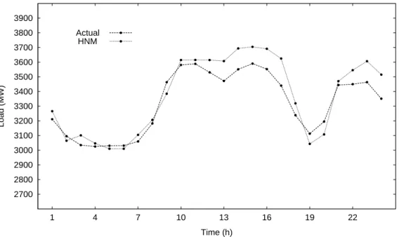
Figure 2: Actual load and forecast load for February 03, 1995
2600 2700 2800 2900 3000 3100 3200 3300 3400 3500 3600 3700 3800
1 4 7 10 13 16 19 22
Load (MW)
Time (h) Actual
HNM
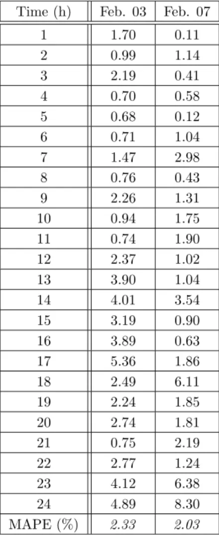
Table 2: Hourly percentage error for February 03 and 07, 1995
Time (h) Feb. 03 Feb. 07
1 1.70 0.11
2 0.99 1.14
3 2.19 0.41
4 0.70 0.58
5 0.68 0.12
6 0.71 1.04
7 1.47 2.98
8 0.76 0.43
9 2.26 1.31
10 0.94 1.75
11 0.74 1.90
12 2.37 1.02
13 3.90 1.04
14 4.01 3.54
15 3.19 0.90
16 3.89 0.63
17 5.36 1.86
18 2.49 6.11
19 2.24 1.85
20 2.74 1.81
21 0.75 2.19
22 2.77 1.24
23 4.12 6.38
24 4.89 8.30
MAPE (%) 2.33 2.03
The training set comprised 2160 load pat-terns, spanning ninety days. The maximum elec-tric load fell around 3900 MWatts. There was no particular treatment for holidays.
Figures 2 and 3 show the actual load and fore-cast load for two particular days. The first one — Friday, February 03, 1995 — is a typical weekday, and the second one — Tuesday, February 07, 1995 — is a special weekday.
A typical weekday is one whose load patterns share some similarity with the load patterns of the same weekdays in former weeks. For instance, the load patterns for Tuesdays tend to display a sim-ilar behaviour. Yet, when an unexpected event, such as a holliday, happens on one of those Tues-days, it changes that fairly stationary behaviour. Such holliday is then said to be a special weekday. Special weekdays break down forecasters, for they perform much better on typical than on special weekdays.
Table 2 presents the performance of the fore-casters for one to twenty-four step ahead predic-tions on those weekdays, as well as the mean ab-solute percentage error (MAPE).
The results from the HNM are very promising. They were compared to the results from a
mul-tilayer perceptron (MLP), working on the same 2160 load patterns (da Silva et al., 2001). Accord-ing to such results, MLP obtained MAPE values of 2.64 and 5.92 for the typical and special week-days respectively.
On the typical day, HNM performed thus bet-ter than MLP. On the special day, the perfor-mance of HNM was significantly superior than that of MLP. The superior performance displayed by HNM seems to be justified by its superior ca-pacity to encode context information from load series in time, and to memorize that information in order to produce better forecasts.
The forecasting errors were fairly high, how-ever, even for the HNM model. The load pat-terns were divided into seven groups, each one corresponding to a specific weekday. An analysis of those groups of patterns was then performed. It was observed that the training patterns within each group did not share much similarity between themselves. More, the difference was significant when comparing them with the testing patterns. Another Brazilian electric utility was contacted to provide us with more relevant and enlarged se-quences of load data.
6 Conclusion
The paper presents a novel artificial neural model for sequence classification and prediction. The model has a topology made up of two self-organizing map networks, one on top of the other. It encodes and manipulates context information effectively.
The results obtained have shown that the HNM was able to perform efficiently the predic-tion of the electric load in both very short and short forecasting horizons. Furthermore, the re-sults are better than those obtained by MLP on equal data.
It is worth mentioning that MLP has been widely employed to tackle the problem of STLF so far. The results obtained thus suggest that HNM may offer a better alternative to approach such problem.
A research and development project for a Brazilian electric utility is under course. The re-search will focus on the effects of the HNM time integrators on the predictions in order to produce a better adaptability. Besides, it will focus on the study of its performance on larger load databases. The forecasts should also span a larger number of days in order to be more significant statistically.
Acknowledgements
References
Bakirtzis, A., Petridis, V., Klartzis, S., Alexiadis, M. and Maissis, A. (1996). A neural net-work short-term load forecasting model for the Greek power system, IEEE Trans. on Power Systems11(2): 858–863.
Carpinteiro, O. A. S. (1997). A hierarchical self-organizing map model for pattern recogni-tion,inL. Caloba and J. Barreto (eds), Pro-ceedings of the Brazilian Congress on Artifi-cial Neural Networks 97 (CBRN 97), Flori-an´opolis, SC, Brazil, pp. 484–488.
Carpinteiro, O. A. S. (1998). A hierarchi-cal self-organizing map model for sequence recognition, in L. Niklasson, M. Bod´en and T. Ziemke (eds),Proceedings of the Interna-tional Conference on Artificial Neural Net-works 98, Sk¨ovde, Sweden, pp. 815–820.
Carpinteiro, O. A. S. (2000). A hierarchi-cal self-organizing map model for sequence recognition,Pattern Analysis & Applications 3(3): 279–287.
Chappell, G. J. and Taylor, J. G. (1993). The tem-poral Kohonen map,Neural Networks6: 441– 445.
da Silva, A. P. A., Reis, A. J. R., El-Sharkawi, M. A. and Marks, R. J. (2001). Enhanc-ing neural network based load forecastEnhanc-ing via preprocessing,Proceedings of the Interna-tional Conference on Intelligent System Ap-plication to Power Systems, Budapest, Hun-gary, pp. 118–123.
Hippert, H., Pedreira, C. and Souza, R. (2001). Neural networks for short-term load forecast-ing: A review and evaluation, IEEE Trans. on Power Systems16(1): 44–55.
James, D. L. and Miikkulainen, R. (1995). SARD-NET: a self-organizing feature map for se-quences, inG. Tesauro, D. S. Touretzky and T. K. Leen (eds),Proceedings of the Advances in Neural Information Processing Systems, Vol. 7.
Kangas, J. (1994). On the Analysis of Pattern Sequences by Self-Organizing Maps, PhD the-sis, Laboratory of Computer and Information Science, Helsinki University of Technology, Rakentajanaukio 2 C, SF-02150, Finland.
Khotanzad, A., Afkhami-Rohani, R. and Maratukulam, D. (1998). ANNSTLF – artificial neural network short-term load forecaster – generation three, IEEE Trans. on Power Systems13(4): 1413–1422.
Khotanzad, A., Hwang, R., Abaye, A. and Maratukulam, D. (1995). An adaptive modu-lar artificial neural hourly load forecaster and its implementation at electric utilities,IEEE Trans. on Power Systems10(3): 1716–1722. Kohonen, T. (2001). Self-Organizing Maps, third
edn, Springer-Verlag, Berlin.
Lee, K., Cha, Y. and Park, J. (1992). Short-term load forecasting using an artificial neu-ral network,IEEE Trans. on Power Systems 7(1): 124–132.
Liu, K., Subbarayan, S., Shoults, R., Manry, M., Kwan, C., Lewis, F. and Naccarino, J. (1996). Comparison of very short-term load forecasting techniques, IEEE Trans. on Power Systems11(2): 877–882.
Lo, Z. and Bavarian, B. (1991). Improved rate of convergence in Kohonen neural network, Proceedings of the International Joint Con-ference on Neural Networks, Vol. 2, pp. 201– 206.
Mohammed, O., Park, D., Merchant, R., Dinh, T., Tong, C., Azeem, A., Farah, J. and Drake, C. (1995). Practical experiences with an adap-tive neural network short-term load forecast-ing system, IEEE Trans. on Power Systems 10(1): 254–265.
Mori, H. (1996). State-of-the-art overview on ar-tificial neural networks in power systems, in M. El-Sharkawi and D. Niebur (eds), A Tu-torial Course on Artificial Neural Networks with Applications to Power Systems, IEEE Power Engineering Society, chapter 6, pp. 51– 70.
Papalexopoulos, A., Hao, S. and Peng, T. (1994). An implementation of a neural network based load forecasting model for the EMS, IEEE Trans. on Power Systems9(4): 1956–1962. Park, D., El-Sharkawi, M., Marks II, R., Atlas,