Universidade de Aveiro Departamento deElectrónica, Telecomunicações e Informática, 2016
Filipe
Teixeira
Boosting Compression-based Classifiers for
Authorship Attribution
Atribuição de Autoria com Boosting de
Classificadores baseados em Compressão
Universidade de Aveiro Departamento deElectrónica, Telecomunicações e Informática, 2016
Filipe
Teixeira
Boosting Compression-based Classifiers for
Authorship Attribution
Atribuição de Autoria com Boosting de
Classificadores baseados em Compressão
Dissertação apresentada à Universidade de Aveiro para cumprimento dos requisitos necessários à obtenção do grau de Mestre em Engenharia de Com-putadores e Telemática, realizada sob a orientação científica do Prof. Dr. Armando Pinho, Professor do Departamento de Eletrónica, Telecomuni-cações e Informática da Universidade de Aveiro
o júri / the jury
presidente / president Prof. Dr. Ana Maria Perfeito Tomé Professora Associada da Universidade de Aveiro Associate Professor at the University of Aveiro
vogais / examiners committee Prof. Dr. Bernardete Martins Ribeiro
Professora Associada com Agregação da Universidade de Coimbra Associate Professor with Habilitation at the University of Coimbra
Prof. Dr. Armando José Formoso de Pinho
Professor Associado com Agregação da Universidade de Aveiro (orientador) Associate Professor with Habilitation at the University of Aveiro (advisor)
agradecimentos / acknowledgements
Agradeço ao Prof. Dr. Armando J. Pinho pelo acompanhamento e liberdade que me permitiu ao longo deste trabalho.
Resumo Atribuição de autoria é o ato de atribuir um autor a documento anón-imo. Apesar de esta tarefa ser tradicionalmente feita por especialistas, muitos novos métodos foram apresentados desde o aparecimento de computadores, em meados do século XX, alguns deles recorrendo a compressores para encontrar padrões recorrentes nos dados. Neste trabalho vamos apresentar os resultados que podem ser alcançados ao utilizar mais do que um compressor, utilizando um meta-algoritmo conhecido como Boosting.
Abstract Authorship attribution is the task of assigning an author to an anony-mous document. Although the task was traditionally performed by expert linguists, many new techniques have been suggested since the appearance of computers, in the middle of the XX century, some of them using compressors to find repeating patterns in the data. This work will present the results that can be achieved by a collaboration of more than one compressor using a meta-algorithm known as Boosting.
Contents
Contents i
List of Figures iii
List of Tables v
List of Abbreviations vii
List of Notation ix 1 Overview 1 1.1 Authorship Attribution . . . 2 1.2 Information Theory . . . 4 1.3 Data Compression . . . 6 1.3.1 Huffman Coding . . . 6 1.3.2 Arithmetic Coding . . . 8 1.3.3 Compression Models . . . 9 1.4 Compression-based Methods . . . 11 1.5 Dataset . . . 13 2 Classifiers 17 2.1 Similarity Measures . . . 18
2.1.1 Normalized Compression Distance . . . 18
2.1.2 Conditional Complexity of Compression . . . 19
2.1.3 Normalized Conditional Compression Distance . . . 20
2.1.4 Normalized Relative Compression . . . 20
2.2 Compressors . . . 21
2.3 Text Length Normalization . . . 23
2.4 Evaluation Methods . . . 24
2.4.1 Maximum Similarity . . . 26
2.4.2 Equal Voting . . . 28
2.4.3 Author’s Average . . . 31
2.5 Comparing Results and Conclusions . . . 34
3 Committees 37 3.1 Voting . . . 38
3.2 Averaging . . . 39
3.3 Weighting . . . 40
3.3.1 AdaBoost and AdaBoost.M2 . . . 41
3.3.2 AdaBoost.M2 for compression based classifiers . . . 45
4 Conclusion 49 4.1 Future Work . . . 49
Bibliography 51
A Processing times for AMDL, SMDL and BCN 55
List of Figures
1.1 Tree generated by Huffman’s algorithm. . . 7
1.2 Arithmetic encoding abab. . . . 8
1.3 Decoding Lempel Ziv [D=11,L=21] using the LZ77 algorithm. . . . 9
1.4 Assigning a target’s author using a set of reference documents. In the figure, ri is a reference document and siis the similarity between ri and the target. . . 12
1.5 Varela’s document lenght distribtuion. . . 14
1.6 Maximum profile sizes by author. . . 15
2.1 Process of classifying a target document. . . 17
2.2 Problem with simple truncation. . . 24
2.3 Percentage of tests for which at least one correct reference was found in the top x% of the references sorted by distance. . . 25
2.4 Distances achieved for a simplified example where N = 3 captures the correct author. 29 2.5 Distances achieved for a simplified example where N = 1 captures the correct author. 29 2.6 Distances achieved for a simplified example where N = 5 captures the correct author. 29 2.7 Comparing the best equal voting classifier with the upper bound. . . 30
2.8 The problem with ignoring distances. . . 31
2.9 Selecting author by using the Author’s Average. . . 32
2.10 Comparing C1and C2 with their upper bounds. . . 33
3.1 Disjunction of all results by classifiers without evaluation methods. . . 38
3.2 Performances achieved by all classifiers compared to Equal Voting. . . 38
3.3 Behavior of AdaBoost’s weight function . . . 42
3.4 Behavior of AdaBoost.M2 weight function . . . 44
3.5 Weights assigned to classifiers by AdaBoost.M2. . . 46
3.6 Performances achieved vs. weight assigned. . . 46
3.7 Performances achieved by all classifiers and committees. . . 48
List of Tables
1.1 Authorship Attribution results achieved in the literature [1]. . . 3
1.2 Results achieved in Varela’s dataset. . . 4
1.3 Context counts example. . . 10
1.4 Partial matching context example. . . 11
1.5 Compression time for different amounts of random data. . . 13
1.6 Varela’s descriptive statistics. . . 14
2.1 Options used with CondCompNC. . . 21
2.2 Average compressed lengths and standard deviations of 10000 bit random strings. . 22
2.3 Compressed lengths of x and xx. . . 22
2.4 Compressed lengths of x, y and xy. . . 22
2.5 Summary of compressor’s quality. . . 23
2.6 Summary of compressor’s quality. . . 23
2.7 Example of the proportional truncation algorithm. . . 25
2.8 Illustrative example of the limitations of an evaluation method. . . 26
2.9 Best results from classifiers using Maximum Similarity as their evaluation method. . 27
2.10 Results by theme from the best classifiers using Maximum Similarity as their evalu-ation method. . . 27
2.11 Confusion Matrix of the results achieved by (CCC, PPMd, True, True) with Maxi-mum Similarity. . . 28
2.12 Results from some classifiers using Maximum Similarity as their evaluation method. 28 2.13 Best results from classifiers using Equal Voting, with N votes, as their evaluation method. . . 30
2.14 Results by theme from the best classifiers using Equal Voting, with N = 3, as its evaluation method. . . 30
2.15 Confusion matrix of the results achieved by the best classifier with Equal Voting and
N = 3. . . 31
2.16 Results from some classifiers using Author’s Average, with N references, as their eval-uation method. . . 32
2.17 Results by theme from the best classifiers using Author’s Average, with N = 3, as its evaluation method. . . 33
2.18 Confusion Matrix of the results achieved by (CCC, PPMd, False, False) with Author’s Average and N = 3. . . 33
2.19 Results from the best classifier from each evaluation method. . . 34
2.20 Average performance achieved by each similarity measure. . . 34
2.21 Average performance achieved by each compressor. . . 34
2.22 Average performance achieved by concatenating references. . . 35
2.23 Average performance achieved by normalizing references. . . 35
2.24 Average performance achieved by each evaluation method. . . 35
2.25 Average results by theme from the three best classifiers. . . 35
3.1 Upper-bound established by the disjunction of all classifiers. . . 38
3.2 Results by theme from a committee with 96 classifiers mixed by equal voting. . . 39
3.3 Results by theme from a committee with 96 classifiers mixed by averaging. . . 40
3.4 Results by theme from a committee with 96 classifiers mixed by AdaBoost.M2 . . . . 47
3.5 Confusion Matrix of the results achieved by AdaBoost.M2 with 96 classifiers. . . 47
3.6 Performance achieved by using a different number of classifiers in the committee. . . 48
A.1 Comparing processing times for SMDL, AMDL and BCN. . . 56
List of Abbreviations
• RLE: Run-Length Encoding • LZ77/LZ78: Lempel-Ziv 77/78
• LZMA: Lempel–Ziv–Markov chain algorithm • PPM: Prediction by Partial Matching
• RAR: An archive file format, stands for Roshal Archive • Gzip: GNU zip
• PNG: Portable Network Graphics
• JPEG: Joint Photographic Experts Group • FLAC: Free Lossless Audio Codec
• MP3: MPEG-1 (or 2) Audio Layer 3 • H.264: Video compression standard
• SMDL: Standard Minimum Description Length • AMDL: Approximate Minimum Description Length • BCN: Best-Compression Neighbor
• NID: Normalized Information Distance • NCD: Normalized Compression Distance • CCC: Conditional Complexity of Compression
• NCCD: Normalized Conditional Compression Distance • NRC: Normalized Relative Compression
List of Notation
• σ: Standard Deviation. • A: The average value of A.
• |x|: The number of elements in x, if x is a set, or the lenght of x if x is a string. • x· y: The concatenation of y to x.
• H(X): Shannon’s entropy of a random variable, X. • K(x): Kolmogorov’s complexity of a document, x.
• K(x|y): Conditional Kolmogorov’s complexity of x given another document, y. • C(x): The length of a document, x, after being compressed by a compressor C. • C(x|y): The compressed length of x by the compressor C using also the models of y. • C(x||y): The compressed length of x by the compressor C using only the models of y. • (Sim. Metric, Compressor, Concatenation, Normalization, Eval. Method): The format used
to represent the components of a classifier, e.g. (NCD, Gzip, False, False, Max. Similarity). Sometimes Eval. Method is omited.
Chapter 1
Overview
Idiolect is defined as “the speech of an individual, considered as a linguistic pattern unique among speakers of his or her language or dialect”1 or “a person’s individual speech habits”2. If each person
has indeed an unique idiolect, studying a text’s patterns allows an expert, or algorithm, to attribute an anonymous document to a known author, i.e, an author with known and undisputed reference documents. The study of style in a language has its own field, known as stylometry.
Stylometry is traditionally applied by an expert, that decides which features are relevant to dis-tinguish between different classes (such as languages or authors) and then evaluates them, with some common features being sentence lengths or repetitions of common words like “the” and “to”. An alternative method was presented in 2002 in [2], that relies on data-compression to recognize the rel-evant patterns. Since then, several variations have been developed and some of them can be applied with well known off-the-shelf compressors, such as Zip, RAR or 7z. By giving the task of pattern finding to the compressor, this method doesn’t require fine-tuning by an expert, who only has to choose which compressor to use.
In this work, we address the problem of Authorship Attribution stylometricly, by considering only the contents of the texts themselves, ignoring other important features such as calligraphy or historical data. This makes the work developed suitable to be applied in contexts where there’s no access to information besides the contents of the document, a common situation in digital media. Furthermore, only compression-based methods will be studied, testing new compressors and then presenting a slight variation on the method, by combining more than one. In the next sections,
1American Heritage® Dictionary of the English Language, Fifth Edition. (2011) 2-Ologies & -Isms. (2008)
authorship attribution will be better defined, followed by a short history of the field and the state of the art. After that, the theoretical foundations and used dataset will be presented. The two main chapters will start by trying to replicate previous work, in order to establish base results, and then new variations will be tried and their results compared. In the end, some conclusions will be presented and future work suggested.
1.1
Authorship Attribution
Authorship Attribution can be defined as the process of inferring some of the author’s features, like age, gender or name, from a document produced by him. Recently, computational or statistical methods have been developed, focusing mostly on distinguishing between candidate authors, i.e., selecting the most likely author amongst a group of probable authors. Some of the other related research topics can be grouped into three classes:
• Profiling: Identifying certain characteristics of the author such as gender, age or date of writing [3, 4, 5, 6, 7, 8, 9]. Useful if there isn’t a set of likely authors.
• Verification: Confirming that a text was written by a given person [10, 11, 12]. Useful for detecting plagiarism.
• Consistency: Confirming that a set of texts were all written by the same person [13, 14]. Useful for detecting tampering.
One of the earliest examples of studying language to identify the author of a document occurred in 1439, when Lorenzo Valla, a priest for the Catholic Church, identified that the Donation of
Constan-tine was a forgery, used by the papacy to gain authority over territory from the Roman Empire [15].
Valla concluded that the document, claimed to have been written in the 4th century, used language from the 8th century. Another well known application of linguistics was made by Thomas Corwin Mendenhall, who published in 1887 studies about the frequency distribution of word’s lenghts in documents by different authors. A few years later, in 1901, he applied his techniques to works of Shakespeare, Bacon and Marlowe, in an attempt to settle a claim that some of Shakespeare’s texts were in fact written by Bacon or Marlowe [16]. In the end, Mendenhall concluded that it was very unlikely that Shakespeare wasn’t the real author. However, his conclusions were contested in 1975 by C. B. Williams [17]. Similar work was done by Cyrus Hoy in 1956, who used the frequency of short words such as ye, hath or them to distinguish the authorship of plays published in the 16th and 17th centuries by John Fletcher, Francis Beaumont and Philip Massinger.
In the end of the 19th century, in 1890, Wincenty Lutosławski, a Polish philosopher, coined the term Stylometry and published the book Principes de stylométrie, setting the basic ideas of the field and using his ideas to establish the chronology of Plato’s documents. Later, in the first half of the 20th century, studies in statistics by George Kingsley Zipf and Udny Yule helped develop the field of statistics and provided important tools for authorship identification, such as using Zipf ’s Law to create an author’s signature distribution [18].
Perhaps the most relevant case for today’s authorship attribution was the study of the Federalist
Papers, in 1964. In it, Mosteller and Wallace tried to identify the author of 12 out of 85 anonymously
published essays texts in 1787-1788 that were claimed by both Alexander Hamilton and James Madi-son. Mosteller and Wallace applied for the first time both Bayesian statistics and computers to the problem, initiating the nontraditional approaches that have mostly been used since. After that, many approaches have been proposed, including neural networks, support vector machines, naive Bayes and many others [19].
The results obtained in different studies depend greatly on the dataset and evaluation used. Even so, Table 1.1 shows some of the results published between 2002 and 2011.
Classifier Database Correct classifications(%)
SVM Web pages 66–80
SVM German newspaper 80 SVM 3 sister’s letters 75
kNN Novels 66–76
Distance Brazilian novels 78 SVM Brazilian newspaper 72 Bayes Mexican Poems 60–80 Bayes Turkish newspaper 80 SVM Brazilian newspaper 74
Table 1.1: Authorship Attribution results achieved in the literature [1].
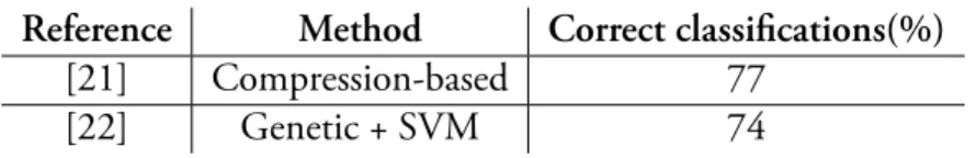
As can be seen in the table, the best results in the field are able to correctly classify approximately 80% of the texts. Some authors have published results of 100% using smaller datasets, such as [20] where the authors used a dataset with 168 documents classified with a compression-based method. In this work, Varela’s dataset will be used ( presented in Section 1.5 bla). Some results have been published with this dataset (Table 1.2) and the achieved performances are similar to other datasets.
Although authorship attribution is not yet ready to be a strong evidence in a dispute, with the best results misclassifying one document out of every four or five, they can already be used to provide
Reference Method Correct classifications(%)
[21] Compression-based 77 [22] Genetic + SVM 74
Table 1.2: Results achieved in Varela’s dataset.
support to other arguments.
1.2
Information Theory
In this work, the term information will be used frequently and as such it should be properly defined. Two such definitions exist, related to Shannon’s Entropy and to Kolmogorov’s Complexity. Claude Shannon published his definition of information theory in 1948 [23], providing a mea-surement, in bits, of the average amount of information that a source of symbols conveys, or has he called it, entropy. Shannon’s entropy is defined for a random variable X taking values (messages) x out of a finite or countable setX
H(X) =∑ x∈X pxlog2 1 px , (1.1)
where px = P (X = x). Notice that if all messages have the same probability, H(X) = log2(|X |),
where |X | represents the cardinality of X . This means Shannon’s entropy does not measure how much information is intrinsically in x, but how much information is required to distinguish between the values inX . Equation 1.2 illustrates this point in an example where all messages are equally likely.
H({’yes’, ’no’}) = H({War and Peace by Leo Tolstoy, Ulysses by James Joyce}) = log2(2) = 1 (1.2) Motivated by Shannon’s entropy inability to measure the information in an isolated document, Kolmogorov proposed a different measurement, now known as the Kolmogorov Complexity. Quot-ing from [24]:
Our definition of the quantity of information has the advantage that it refers to individual objects and not to objects treated as members of a set of objects with a probability distribution
given on it. The probabilistic definition can be convincingly applied to the information contained, for example, in a stream of congratulatory telegrams. But it would not be clear how to apply it, for example, to an estimate of the quantity of information contained in a novel or in the translation of a novel into another language relative to the original. I think that the new definition is capable of introducing in similar applications of the theory at least clarity of principle.
Strings like aaa...aaa can easily be represented by short programs in most languages. Likewise, seemingly complex numbers like π can be printed up to any arbitrary number of digits by short computer programs, meaning that both examples have very little information despite their length.
Kolmogorov’s complexity is an absolute quantification of the information in a document x, K(x), and defines it as the length of a smallest possible description of x using any universal language, such as a Turing Machine or a programming language like Java or C. By knowing the encoding algorithm x can be completely retrieved from its description. Unfortunately, it’s not computable for an arbitrary document. Formally, Kolmogorov’s complexity is defined in (1.3), whereU represents a universal Turing machine and p a program written in some language.
KU(x) =min
p {|p| : U(p) = x} , s (1.3)
where|p| represents the length, number of bits, of p. The choice of U is not important, since they differ only by up to some constant, the size of a program that translates between languages [25].
Another related definition, crucial for the field of compression-based similarity, is the conditional Kolmogorov complexity, K(x|y), where y is another document. Conditional complexity measures how much information is in x that isn’t in y, i.e., measures the size of the smallest program that can mutate y into x. Using a Turing machine that performs such a task,U(p, y) = x, conditional complexity is defined by
KU(x|y) = min
p {|p| : U(p, y) = x} . (1.4)
This measurement can reveal how much information two documents share or by how much they differ. If y is an empty string, K(x|y) = K(x). Although not computable, Kolmogorov’s complexity provides useful notions about information and it can be approximated, from above, using a general purpose data compressor, C. That upper-bound is defined in (1.5), where C(x) is the length of x
after being compressed by C and|DC| is the length of a program able to decompress data compressed
by C.
K(x)≤ C(x) + |DC| (1.5)
Using a compressor as an approximation to Kolmogorov’s complexity is used throughout this work, and as such some common compression algorithms will be presented in the next section.
1.3
Data Compression
In the last section, we’ve seen that any general purpose data compressor can be used to estimate the uncomputable Kolmogorov Complexity. Data compression is the process of representing data with fewer bits than the original. In other words, if C is a data compressor, then for some x’s, C(x)≤ |x|, where x is a string of|x| bits and C(x) is the length of the representation of x given by C.
There are two approaches for compression, known as lossy and lossless, both widely used. The first tries to represent the most important features of the original data, losing information that is thought to be less important. These are mostly used in media codecs such as JPEG, for pictures, MP3, for audio, and H.264 for video. As the name implies, lossless compression preserves all the information in the original data and is used in general purpose compressors such as Gzip or RAR and also in some media formats like PNG and FLAC. This section will only approach the latter as only those will be used in the thesis.
A compression algorithm has two components: a model and a coder. The model is responsible for finding patterns in the data and capturing the probability distribution of symbols or segments of the message, allowing it to make predictions on what the remaining message should be. The coder uses that information and represents it in as little bits as possible, for example by assigning a shorter or longer identifier for symbols based on their probability, with common strings having the shorter ones. Although many different models exist, most algorithms use either Huffman or Arithmetic coders.
1.3.1
Huffman Coding
Huffman coding was developed by David Huffman in 1950, and has been shown to produce optimal prefix codes, i.e. represents any probability distribution in the least amount of bits using
a prefix code. A prefix code is a type of uniquely decodable code where no identifier is a prefix of another, for example: {(a:1), (b:01), (c:001), (d:000)}. The technique proposed by Huffman is shown in Algorithm 1.1.
Data: A probability distribution of all messages.
Result: The code, or identifier, assigned to each message.
Start with one node for each message, with the associated probability
while Number of nodes is larger than 1 do
Select the two nodes with smallest probabilities
Combine them into a child node, with it’s probability being the sum of their probabilities
end
Algorithm 1.1: Huffman coding algorithm.
Algorithm 1.1 builds a binary tree, where each message is represented by a leaf node, that can be used to generate the code by assigning some symbol to both child nodes, for example 1 for the left child and 0 for the right. As an example, consider that the messages to be transmitted are {(a:50%), (b:25%), (c:12.5%), (d:12.5%)}. Following the algorithm, the result is the tree in Figure 1.1.
100% 50% 25% 12.5% d 12.5% c 25% b 50% a 0 1 0 1 0 1
Figure 1.1: Tree generated by Huffman’s algorithm.
Starting at the root note, 100%, the path to each leaf determines the code of the message, obtain-ing the same code presented before: {(a:1), (b:01), (c:001), (d:000)}. Usobtain-ing this encodobtain-ing, an average message that follows the same distribution would require 1.75 bits per character, instead of 2.
1.3.2
Arithmetic Coding
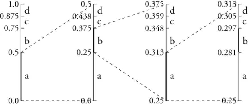
Although Huffman codes are optimal prefix codes, prefix codes are themselves inefficient relative to the entropy. Arithmetic coding improves on this by sharing some bits to represent more than one symbol in the message, by encoding a message as an interval in the number line between 0 and 1. The algorithm is presented in Algorithm 1.2.
Data: A probability distribution of all messages and a sequence, s, to encode. Result: The code assigned to s.
remaining = s, min = 0.0, max = 1.0
while length of remaining > 0 do
Split the interval [min, max) using the probability distribution Select the first symbol, c, from remaining
Set min and max to the interval endpoints of c Remove c from remaining
end
Algorithm 1.2: Arithmetic coding algorithm.
The final values of min and max encode the given sequence, which can be simplified into any value from the interval and the length of the sequence. Using the same probability distribution as the example in the previous section, Figure 1.2 illustrates the algorithm with rounded values.
a b c d 0.0 0.5 0.75 0.875 1.0 a b c d 0.0 0.25 0.375 0.438 0.5 a b c d 0.25 0.313 0.348 0.359 0.375 a b c d 0.25 0.281 0.297 0.305 0.313
Figure 1.2: Arithmetic encoding abab.
The figure shows that abab can be encoded by the interval [0.2813, 0.2969), or alternatively by a value from the interval and the length of the sequence, for example (0.29, 4).
1.3.3
Compression Models
This section presents some of the most well known compression models. A very simple model is known as Run-Length Encoding, or RLE, and replaces adjacent repetitions of a value by a single instance of the value and a count of repetitions:
‘RRRRRRRRRRLLLLLEEEEEEE’ = R10L5E7
In 1977/78 Jacob Ziv and Abraham Lempel jointly purposed two very similar algorithms, later named LZ77 [26] and LZ78 [27], that are able to take advantage of repeating strings, like common words, improving on RLE. They work by finding repeated data in already seen data and replacing new occurrences with a reference, with LZ77 using a pointer to a previous point in the string and LZ78 using dictionary. As an example of compressing a string using LZ77 we have:
‘Lempel Ziv Lempel Ziv Lempel Ziv’ = Lempel Ziv [D=11,L=21],
where D indicates the distance, in characters, where that string was last seen, and L the number of characters to be repeated. The process followed to recover the original message is illustrated in Figure 1.3, where & symbolizes the pointer [D=11,L=21].
1 2 3 4 5 6 7 8 9 10 11 12 13 14 15 16 17 18 19 20 21 22 23 24 25 26 27 28 29 30 31 32
L e m p e l Z i v &
L e m p e l Z i v L e m p e l Z i v L e m p e l Z i v
-11 -11
Figure 1.3: Decoding Lempel Ziv [D=11,L=21] using the LZ77 algorithm.
The data is decompressed in order, from the beginning to the end, allowing L to be larger than D. If this was not the case, the 23rd character from the example wouldn’t be recoverable. Because
LZ78 uses an explicit dictionary this limitation is not present, and any segment of the data can be de-compressed without decompressing what came before. Due to computational limitations, LZ77 only looks for identical segments in the most recent k characters, which defines a window of k characters that can be used to compress new data. As such, LZ77 is known as a sliding window algorithm. A popular available compressor that uses LZ77 is gzip, which sets it’s maximum window size to 32kB. Variations of the Lempel-Ziv algorithms include Lempel-Zip-Markov chain (LZM), a modification of LZ77 used by 7z and LZMA, and Lempel-Ziv-Welch (LZW) based on LZ78 and used by GIF and compress program available in Unix and FreeBSD.
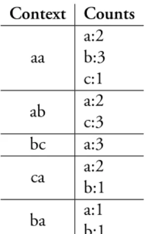
Another approach to data compression uses the probability of each character to minimize the length of the most common. A compressor that yields the one of the best compression ratios is PPM, or Prediction by Partial Matching. PPM uses the last k characters to estimate a conditional probability of the next character, achieving this by storing a dictionary with counts of what was found until then. Table 1.3 shows an example of the table built after processing the string aabcabcaaababcaaabaac with
k = 2. Context Counts aa a:2 b:3 c:1 ab a:2 c:3 bc a:3 ca a:2 b:1 ba a:1 b:1
Table 1.3: Context counts example.
Using this information table, the following character can be encoded, usually using arithmetic coding, in a smaller number of bits. Because this table only depends on previous information, the decompression process can rebuild the probability distribution and arrive at the same code, which is then used to decode the current symbol.
The partial matching, in PPM, refers to the way the algorithm deals with the case when the current context has never been observed, for example if the next character in the above string was an a. Instead of using a dictionary with all the k characters strings found, PPM stores k different dictionaries, keeping counts for contexts of lengths 0, 1 . . . k. Using the same string as above, the resulting dictionaries are shown in Table 1.4.
Because the probability of a character x given the context s is given by P (x|s) = C(x|s)/C(s), where C(s) is the number of times s was counted and C(x|s) the count of finding x after s, and larger contexts appear less often than shorter ones, using as large a context as possible increases the probabilities of finding x. As we’ve seen in the previous section the more likely a message is the less bits are required to transmit it. Due to this, PPM always tries to encode a message using the largest context possible.
Many compressors use this or other statistical methods. Of them, PPMd and CondCompNC
Context (k=0) Counts Context (k=1) Counts Context (k=2) Counts None a:12 b:5 c:4 a a:6 b:5 aa a:2 b:3 c:1 b a:2 c:4 ab a:2 c:3 c a:3 bc a:3 ca a:2 b:1 ba a:1 b:1
Table 1.4: Partial matching context example.
were selected to be used in this work. Other techniques, and combinations of them, exist but this section intended only to present some of the ideas of the field. In the next section we’ll see how compressors can be used in authorship attribution.
1.4
Compression-based Methods
As mentioned earlier, compression-based methods rely on compressors to find important patterns in the data, providing a numerical measurement to the similarity between them. These methods require a set of reference documents, whose authorship is accepted as true, with samples from all possible authors. A new document is then compared to the references and the most similar reference assigns the author of the new text.
The main concept with this approach is to let a compression algorithm retrieve the most relevant information from reference documents, and then use the same algorithm to compress a target docu-ment using the information of the reference. Similarity between a reference and a target should yield better compression rates.
Overall, compression-based methods use a set of reference documents, R, to classify a target, t. Using the compressor, it computes the similarity between t and r ∈ R, and then assigns the author of t to be the author of the most similar reference. The process is illustrated in Figure 1.4.
Marton et al. [28] distinguish between three distinct procedures, SMDL, AMDL and BCN. Standard Minimum Description Length, or SMDL, generates a compression model for each class, usually by concatenating all references within the same class and then extracting the models for each
r0 r1 r2 Compute Similarities Target s0 s1 s2
Maximum Similarity Author
Figure 1.4: Assigning a target’s author using a set of reference documents. In the figure, ri is a
reference document and siis the similarity between riand the target.
concatenated document. That compression model is then used to compress a target document, and the resulting length can be interpreted as a measure of similarity between the target and the refer-ences. Exporting the compression model is not a feature offered by most compressors and AMDL, or Approximate Minimum Description Length, is an alternative method that can be used with any compressor at the cost of time and accuracy. Like SMDL, documents within class i are concatenated into a single document, Ai, with compressed length C(Ai). AMDL then requires the target
doc-ument t to be concatenated at the end of Ai, Ai · t. The compressed length of t using the models
of Ai can be approximated by C(t|Ai) ≈ C(Ai · t) − C(Ai). The last alternative is called
Best-Compression Neighbor, or BCN, a procedure very similar to AMDL, with the only difference being not concatenating the documents within a class, which might make it too sensitive to noise. Us-ing some votUs-ing mechanism can reduce the problem. The methodologies can also be divided into profile-based (SMDL and AMDL), when all the author’s references are concatenated, and instance-based (BCN), with each reference being used individually.
Some criticism of these methods have been expressed, mostly focusing on how slow they are. According to [29] BCN is 17 times slower than Naive-Bayes, a very simple probabilistic classifier, and offers significantly poorer results. These critics have been addressed by Benedetto et al. in [30], claiming that the results presented in [29] were wrong and were published to discredit the approach, when in reality compression-based methods offer comparable results to Naive-Bayes in that specific dataset. Benedetto et al. agreed with the claim that these techniques are slower than other methods, however this can be minimized by using AMDL, reducing the number of compressions needed to the number of classes, and even more by SMDL, removing the need to repeatedly compress all the references when classifying a new document.
Using simple assumptions, it’s trivial to show (Appendix A) that AMDL is between 2 and n + 2 times slower than SMDL and BCN requires 1 to n times more time than AMDL and between 1 and 2n+1than SMDL, where n is the number of references by each author. These results ignore the time required by SMDL to extract the compression models. However this step only happens once and as such is not relevant. In order to validate these approximations, Table 1.5 shows the time required by some compressors to process different amounts of random data. These compressors will be better specified in Section 2.2.
Compressor Time (ms)
100 bytes 1000 bytes 10000 bytes
Gzip 0.17 0.23 0.38
Bzip2 0.11 0.56 3.11
LZMA 22.06 23.44 26.20
PPMd 15.25 14.57 18.49
CondCompNC 11.74 23.31 98.78
Table 1.5: Compression time for different amounts of random data.
The values in Table 1.5 show that the compressors present neither a constant nor a linear process-ing time, but they are both assumptions, with LZMA and PPMd beprocess-ing almost constant and Bzip2 and CondCompNC closer to linear times. The times were measured using different amounts of ran-dom data, and tested up to 10 000 bytes, because the vast majority, 99.8%, of the documents in the dataset are under that size.
1.5
Dataset
In order to evaluate the performance of the methods used further in this work, a set of documents is required. The selected database was originally used by Paulo Varela in [31] and was chosen due to the existence of authorship identification results published by other authors [21][22].
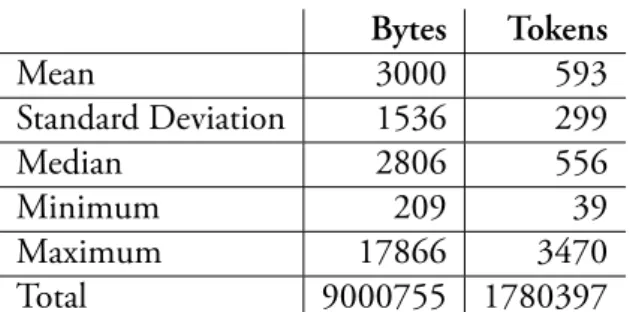
Varela’s dataset has 3000 documents written by 100 authors in Portuguese and collected from different Brazilian newspapers and blogs. It has articles from ten categories: Economy, Gastronomy, Health, Law, Literature, Politics, Sports, Technology, Tourism and Unspecified Subject. Each cat-egory has 300 texts from ten authors, resulting in 30 documents per author. The documents have been used in their original state, without any preprocessing. Some relevant statistics about the corpus can be consulted in Figure 1.6 and Figure 1.5.
5,000 10,000 15,000 0
50 100
Number of Characters (bin size≈ 100)
N
umber
of
D
ocuments
Figure 1.5: Varela’s document lenght
distribtu-ion. Bytes Tokens Mean 3000 593 Standard Deviation 1536 299 Median 2806 556 Minimum 209 39 Maximum 17866 3470 Total 9000755 1780397
Table 1.6: Varela’s descriptive statistics.
The documents are split into two groups, a group of references and a group of targets, used for testing. Following the choices of previous work [21], to facilitate comparisons, seven documents from each author were selected as references and the remaining 23 as test targets, for a total of 700 references and 2300 targets.
Some of the compressors that were used in this work use a sliding window, and only use data inside that window to compress new data. From those, Gzip has the greatest limitation, with a sliding window with a maximum size of 32kB, or 32769 bytes. As such, longer documents will not use the beginning of a document to compress the ending. Although the largest document has 17kB, well below Gzip’s limit, both AMDL and BCN require concatenation of more than one text. Best-Compression neighbor requires two documents, a reference and a target, to be concatenated. If the two largest documents happen to be concatenated, the resulting text would have 31486 bytes, slightly below the limit. However, profile-based procedures require the concatenation of all the author’s references and, as shown in Figure 1.6, a significant number, 30, of the authors may have a larger than the limit profile. The plotted data represents the maximum profile size that each author can have, i.e., the sum of the lengths of it’s seven largest references.
During our work, twelve repeated documents were found in the dataset, lowering the number of different documents to 2988. The repetitions are spread out across some authors: seven authors have 29 unique documents, one has 28 and one has 27. This means that in the case that all repetitions are used as targets and their originals as references, twelve documents are very likely to be correctly classified. However, due to the large number of target documents, the error produced in this worst case would be approximately 0.5%, which is not significant.
After presenting the foundations of the field, the remaining work will start by reproducing other known results, using the same classifiers, and then we’ll study how to combine their results into a
16 32 48 Author P rofile siz e (kibib ytes)
Figure 1.6: Maximum profile sizes by author.
committee, which should be able to provide better results than any single classifier.
Chapter 2
Classifiers
In this work, a classifier is responsible for assigning an author, a ∈ A where A is the set of all authors with reference documents, to a text, using a set of reference documents. After comparing the target to all the references, the classifier selects the author by finding the most similar reference. A classifier has five components:
• Similarity Measure: How to measure the similarity between two texts. • Compressor: What compressor should be used.
• Concatenate: If True, concatenates all texts by the same author.
• Normalize Text Lengths: If True, truncates all documents to the same length. • Evaluation Method: How to interpret the computed similarities.
Target References Preprocessing Concatenate Normalize Compute Similarities Processed References
Compressor Similarity Measure
Similarities
Evaluation Method
Author
Figure 2.1: Process of classifying a target document.
In this chapter, the different components, as well as several combinations, will be addressed.
2.1
Similarity Measures
A similarity measure is a measurement of how similar two separate documents are. Using the no-tions of Kolmogorov Complexity, K(x), and Kolmogorov Conditional Complexity, K(x|y), many alternatives have been purposed in recent years. This first similarity measure, called Normalized In-formation Distance, or NID, is defined as
NID(x, y) = max{K(x|y), K(y|x)}
max{K(x), K(y)} . (2.1)
Although it depends on K(x), and as such it is not computable, it’s still a useful measure, and many compression-based alternatives have been purposed to approximate its results. From the ex-pression, and knowing some properties of Kolmogorov’s complexity, some results can be extracted. Given two identical texts, x ≡ y, K(x|y) = K(y|x) = 0 and NID(x, y) = 0. Given the opposite case, where x and y are completly unrelated, K(x|y) = K(x) and K(y|x) = K(y) and the distance between them is 1. Using compressors to approximate NID should yield similar values.
2.1.1
Normalized Compression Distance
The Normalized Compression Distance, or NCD, was developed [32] as an approximation to NID that uses a compressor as an approximation to the true Kolmogorov Complexity. The distance between the documents x and y computed with the compressor C, is defined as
NCDC(x, y) =
C(x· y) − min{C(x), C(y)}
max{C(x), C(y)} , (2.2)
where C(x) represents the length, in bits, of the document x after being compressed by C and x· y is the concatenation of y to x, i.e, x followed by y, without any connecting characters.
Considering an ideal compressor C, if all the information in x is contained in y, then C(y) ≥
C(x)and C(x· y) = C(y), resulting in a distance of 0. On the other hand, if no information of y can be used to produce x, C(x· y) = C(x) + C(y). Because min{C(x), C(y)} = C(x) implies that max{C(x), C(y)} = C(y), this results in distance of 1. In most cases, however, at least parts of
yare useful to represent x and the NCD returns a value between 0 and 1. As intended, the behavior is identical to NID.
Available compressors, however, are not ideal, resulting in compression lengths greater than Kolmogorov’s complexity. This makes achieving a distance of 0 impossible, because C(x· y) > min{C(x), C(y)}, even if x is perfectly retrievable from y or vice versa.
Many compressors also add extra information, such as checksums and other meta-data. If its size,
ϵ, is constant amongst all compressions, achieving a distance of 1 is also impossible. Consider that the compressor Cϵ requires ϵ bits of meta-data, Cϵ(x) = C(x) + ϵ. Then, the NCD between two
totally different documents, x and y, where C(y) > C(x), is defined as
NCDCϵ =
(C(x) + C(y) + ϵ)− (C(x) + ϵ)
C(y) + ϵ =
C(y)
C(y) + ϵ < 1. (2.3)
The same applies if C(x) > C(y).
Another exception occurs if a classifier, for some reason, compresses a concatenation into a larger file than the sum of the original files, C(x· y) > C(x) + C(y). In this case, the distance would be larger than 1.
2.1.2
Conditional Complexity of Compression
Conditional Complexity of Compression [33], usually CCC, is another commonly used measure. Instead of returning the distance between two documents, it computes the amount of extra infor-mation that is necessary to build the document x from y, i.e. an approxiinfor-mation to Kolmogorov’s conditional complexity:
CCC(x|y) = C(y · x) − C(y). (2.4) Because compressors rely on previously seen patterns to compress new data, by concatenating
xto y, the compressor has already processed y and will use it’s models to compress x. Subtracting
C(y)results in an approximate measure of how much information x contains that was not present in y. Also note that the compressor will also use information from x to compress the remaining data, resulting in a compressed length achieved by using both x and y’s models.
Unlike NCD, CCC is not normalized. Considering again a perfect compressor, if x can be fully assembled with information in y, then C(x· y) = C(y) and CCC(x|y) = 0. On the other extreme,
C(x· y) ≈ C(x) + C(y) and CCC(x|y) ≈ C(x), without any upper bound.
2.1.3
Normalized Conditional Compression Distance
Normalized Conditional Compression Distance is a recent, published in 2014 [34], measurement of the distance between two strings of characters. Unlike the previous measures, NCCD requires a compressor capable of conditional compression, i.e. compressing a document using the models build from another document. Conditional compression, C(x|y), encodes x using models build from both y and x, similarly to CCC(x|y). As such, C(x|y) represents the number of bits necessary to represent x given the information contained in both x and y. Access to such a compressor allows the creation of a similarity measure very similar to the NID, by simply replacing the Kolmogorov Complexity with a compressor:
NCCDC(x, y) =
max{C(x|y), C(y|x)}
max{C(x), C(y)} . (2.5)
2.1.4
Normalized Relative Compression
The last measure that will be used is called Normalized Relative Compression, a very recent mea-sure published in 2016 [20]. This approach requires a compressor capable of exclusive conditional compression, C(x||y), where x is compressed using exclusively models build from y. This means that information from x isn’t used to compress it and as such, if x and y are completely unrelated,
C(x||y) ≈ |x|. In other words, if y does not contain information relevant to x, x will not be
compressed at all. NRC is defined as
NRCC(x, y) =
C(x||y)
|x| , (2.6)
where|x| is the number of bits necessary to represent x, a string with N symbols out of the set A, without any compression:
|x| = N × log2|A|. (2.7)
As with the other measures, the NRC equals 0 when both documents are identical and 1 if they’re completely different. More generally, NRC ≈ 0 when x can be completely retrieved from y, and NRC≈ 1 when none of x is retrievable from y.
2.2
Compressors
Except for NCCD and NRC, any compressor can be used to compute the similarities. The following have been used in this work:
• Gzip (provided by Python 3.5.1 standard library) • Bzip2 (provided by Python 3.5.1 standard library) • LZMA (provided by Python 3.5.1 standard library) • PPMd (provided by 7z 15.14)
• CondCompNC (version 1.0.0)
These have been selected in an attempt to experiment with a wide variety of compression tech-niques, explained previously in Section 1.3. Except for CondCompNC, the compressors used the highest compression setting available. In order to facilitate replication, the options used to run Cond-CompNC are shown in Table 2.1, where -tt 1:n represents the usage of an order-n finite-context model to model the target, x, and -rt 1:n the same for the reference, y. The value after each model represents the α parameter in (1) of [35]. Note that, unlike conditional compression, exclusive con-ditional compression does not build any models from x to compress it.
Mode Options
C(x· y) -tt 1:2 -tt 1:3 1/10 -tt 1:4 1/100
C(x|y) -rt 1:2 -rt 1:3 1/10 -rt 1:4 1/100 -tt 1:2 -tt 1:3 1/10 -tt 1:4 1/100
C(x||y) -rt 1:2 -rt 1:3 1/10 -rt 1:4 1/100
Table 2.1: Options used with CondCompNC.
As the compressors are being used to approximate Kolmogorov’s Complexity, they should be able to provide approximate values. The following tests were performed with x and y being random strings with 10 000 bits, to represent completely unrelated strings.
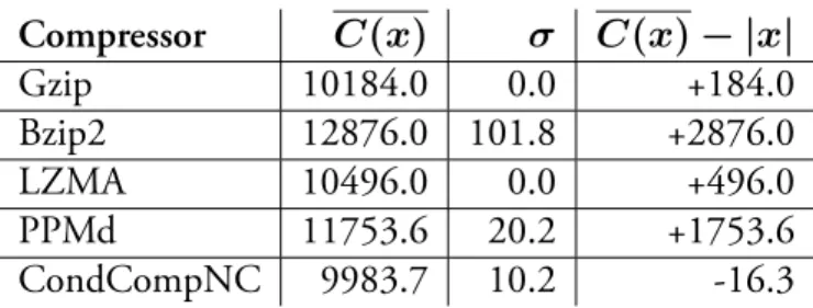
The first test compressed ten random 10 000 bit strings and then averaged their compressed lengths. Assuming a good random number generator, the compressed length should be identical to the uncompressed length. All compressors used the same random strings. The results are in Table 2.2. Both Gzip and LZMA produced compressions with the same length on every string. This suggests that they weren’t able to compress anything on the original strings, and the extra bits are used only for meta-data. The remaining compressors tried to compress the data but resulted in files bigger than the original. The only exception is CondCompNC, that was able to slightly compress a random string, meaning that the string is not truly random. Lengths computed by CondCompNC are also slightly
Compressor C(x) σ C(x)− |x| Gzip 10184.0 0.0 +184.0 Bzip2 12876.0 101.8 +2876.0 LZMA 10496.0 0.0 +496.0 PPMd 11753.6 20.2 +1753.6 CondCompNC 9983.7 10.2 -16.3
Table 2.2: Average compressed lengths and standard deviations of 10000 bit random strings.
lower because CondCompNC does not require any meta-data.
The following test determines how much each compressor can extract from previously seen data, by comparing C(x· x) to C(x). A good compressor should give C(x · x) ≈ C(x). The same conditions were used, 10 repetitions with 10000 bit random strings, and the results are in Table 2.3.
Compressor C(x) C(x· x) ∆ = C(x · x) − C(x) σ∆ Gzip 10184.0 10712.0 528.0 8.0 Bzip2 12911.2 14844.8 1933.6 88.9 LZMA 10496.0 10816.0 320.0 0.0 PPMd 11749.6 15269.6 3520.0 19.6 CondCompNC 9984.6 12275.3 2290.7 5.1
Table 2.3: Compressed lengths of x and xx.
As expected every compressor can use previously seen information to compress new one, however, because these tests used random strings, without any structure or patterns, statistical compressors pro-vide significantly worse results than Lempel-Ziv compressors, which find repeating strings of symbols. Once again LZMA offers very consistent results. The value C(x· x) − C(x) is identical in every test done with this compressor, requiring only 320 to compress the additional 10000 bits.
The final property that should be obeyed by a good compressor processing two unrelated strings is C(x·y) ≈ C(x)+C(y). Using the same conditions as before, the results can be seen in Table 2.4.
Compressor C(x) C(y) C(x· y) ∆ = C(x · y) − (C(x) + C(y)) σ∆
Gzip 10184.0 10184.0 20184.0 184.0 0.0
Bzip2 12896.0 12856.8 23841.6 1911.2 163.6
LZMA 10496.0 10496.0 20480.0 512.0 0.0
PPMd 11752.8 11744.0 22109.6 1387.2 18.7
CondCompNC 9985.3 9986.7 19998.6 -26.6 11.6
Table 2.4: Compressed lengths of x, y and xy.
The results are similar to Table 2.2, with CondCompNC being closest to the ideal value and Bzip2 the farthest. Summing up the results, Table 2.5 shows the difference as a percentage, between each compressor and the optimal values.
Compressor C(x· x) ≈ C(x) C(x · y) ≈ C(x) + C(y) Gzip 5.3% 0.9% Bzip2 19.3% 9.6% LZMA 3.2% 2.6% PPMd 35.2% 6.8% CondCompNC 22.9% -0.1%
Table 2.5: Summary of compressor’s quality.
Overall, the first property is harder, on average, for compressors to follow than the second. LZMA is the compressor that best obeys C(x· x) = C(x) and CondCompNC is able to provide results nearly optimal to C(x· y) = C(x) + C(y).
The remaining desirable properties require a conditional compressor. As such only CondCompNC will be tested. Considering that x and y are two unrelated strings, the properties are:
• C(x||y) ≈ |x| • C(x|y) ≈ C(x) • C(x||x) ≈ 0 • C(x|x) ≈ 0
The results are shown in Table 2.6. As before, they are averaged results from 10 repetitions.
Compressor C(x||y) C(x|y) C(x||x) C(x|x)
CondCompNC 10000 10000 2267.2 2268.2
Table 2.6: Summary of compressor’s quality.
The table shows that for both C(x||y) and C(x|y) this compressor perfectly follows the expected results. Although it was able to use the model learned from x to encode itself, the results achieved are similar to C(x· x), using approximately 2300 bits more than the ideal 0.
2.3
Text Length Normalization
Larger texts usually contain more information, which may result in smaller values for conditional compression, like C(x|y), C(x||y) and CCC(x|y). Due to this, larger references have an higher
chance of being selected as the best match. Normalizing the lengths of the references forces all the texts to have an equal length, and although the discarded text is unused, it solves the bias that compression based classifier may have for larger texts.
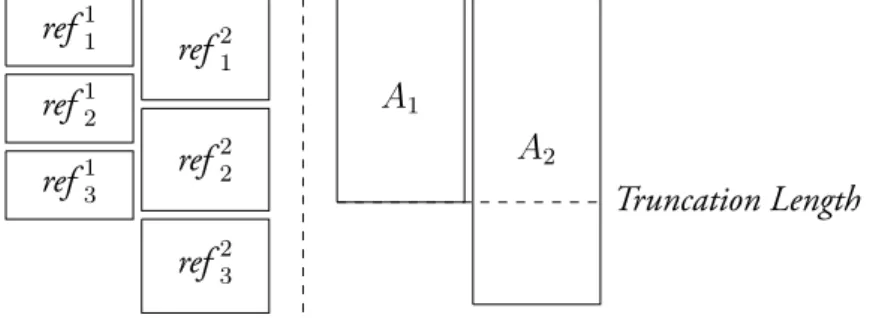
For instance-based classifiers, references can simply be truncated at the length of the shortest reference. However, for profile-based classifiers, the author’s texts are concatenated and an extra step might be useful. If an author as several short texts, their concatenation may be significantly smaller than an author with large texts and simply truncating the concatenated files would erase entire documents from the former, as is illustrated in Figure 2.2, where refab is the the bth reference
of author a. ref11 ref12 ref13 ref21 ref22 ref23 A1 A2 Truncation Length
Figure 2.2: Problem with simple truncation.
A possible approach to avoid losing integral documents is to remove a fraction of the total amount of text to be removed from each reference before concatenating them, resulting in all authors having the same length of reference text. Each document should lose an amount of data proportional to its size. The process used to normalize the references is described in Algorithm 2.1 and an example is given in Table 2.7. As intended, each text loses an identical percentage (20% in the example) of it’s initial length.
2.4
Evaluation Methods
After computing the distances from a target to the references, it’s necessary to select the most likely author, a task that can be approached in multiple ways. Before moving on to the evaluation methods, the previous components can be used to establish limits on what can be achieved in this section. Combining the options presented in previous sections, 48 classifiers can be created. After computing all the distances for the 2300 targets and 700 references, 3 classifiers were selected: one of the best, classifier 1, a median, classifier 2, and one of the worst, classifier 3. Figure 2.3 shows the percentage of tests for which at least one correct reference was found in the top x% of references.
Data: A set of references, R
Result: A new set of truncated references, Rt
Group all texts by the same author, Ga ={r ∈ R|author(r) = a}
Find the author with the minimum sum of text’s lengths, L
for every author a do
Compute the sum of all texts’ lengths in the group, la =
∑
|r|, r ∈ Ga
Compute how much text should be removed from Ga, ∆a = la− L
Compute the proportion of text that should be removed from each referece, pa =∆a/la for every r in Gado
Compute how much text should be removed from r, δr = pa× |r|
Truncate r at len(r)− δr, tr
Add tr to Rt
end end
Algorithm 2.1: Proportional truncation of references.
Required final size: 48 characters
Text’s lenghts: {t1 : 10, t2 : 20, t3 : 30}
Proportions: {t1 :10/60, t2 :20/60, t3 :30/60}
Total data to remove: (10 + 20 + 30)− 48 = 12 Data to remove from each text: δt1 =10/60× 12 = 2
δt2 =20/60× 12 = 4
δt3 =30/60× 12 = 6
Final lengths: {t1 : 8, t2 : 16, t3 : 24} Table 2.7: Example of the proportional truncation algorithm.
0% 10% 20% 30% 40% 50% 60% 70% 80% 90% 100 % 0% 20% 40% 60% 80% 100% References Corr ect Classifications Classifier 1 Classifier 2 Classifier 3 Random Guess
Figure 2.3: Percentage of tests for which at least one correct reference was found in the top x% of
the references sorted by distance.
As an illustrative example of the contents plotted, consider only one classifier, three targets and five references of five authors. After computing the distances and sorting the references for each target from most to least similar, Table 2.8 was built. Each cell represents a reference, and contains a check-mark if it’s a reference by the correct author, a cross otherwise. The references on the left have smaller distances.
Target #1 × ✓ × × × Target #2 ✓ × × × × Target #3 ✓ × × × ×
Table 2.8: Illustrative example of the limitations of an evaluation method.
By looking only at the most similar reference, it’s trivial for classifier 1 to correctly classify 66.6% of the documents. However, by looking at the 2 most similar references, the correct author could be found in 100% of the tests. This would require some evaluation method capable of perfectly selecting the correct author of each target, but in any case it sets an upper limit on how well any evaluation method can perform by using the N best references and shows that the ranked list, as a hole, contains more relevant information than just the top reference.
In Figure 2.3, the x axis uses a percentage, as opposed to an absolute value, because, depending on whether the classifier is instance or profile-based a different number of references may exist. By using a percentage they can be plotted together and their results more easily compared. Also note that only evaluation methods that make use of a large portion of references are able to achieve performances near 100%, i.e. correctly classify every target document. The evaluation methods that will be presented in this section assume that the distances between documents have already been computed, resulting in a sorted list of distances from a target t to each reference r ∈ R, defined as:
Dt= (da1, db2, dc3, . . . dr|R|) : a, b, c, r ∈ R, (2.8)
where d1is the smallest distance and corresponds to the distance between t and a.
2.4.1
Maximum Similarity
Maximum Similarity is the simplest strategy. Given Dt, assign the author of a, with distance
da
1, as the author of the target document. The three best results achieved by this method are in
Table 2.9. Note that, because there are 100 authors in this dataset, a random guess classifier would offer a performance of 1%.
Measure Compressor Concatenate Normalize Correct classifications
CCC PPMd True True 68.87%
NCD PPMd False False 68.39%
NCD Gzip False False 68.04%
Table 2.9: Best results from classifiers using Maximum Similarity as their evaluation method.
Due to the large number of authors presenting results for each one, individually, is impractical. Grouping the tests by category provides a good balance and allows for some more insight into the results. For clarification, the targets are still classified by the author, not the theme. Table 2.10 shows the percentage of correctly classified authors for targets in a given theme.
Category C1 C2 C3 Economy 69.87% 66.38% 70.74% Gastronomy 61.57% 51.09% 48.91% Health 69.57% 67.83% 67.39% Law 72.81% 63.60% 64.06% Literature 56.58% 52.63% 51.32% Politics 66.09% 76.09% 71.30% Sports 73.48% 76.09% 76.96% Technology 80.87% 78.26% 78.26% Tourism 72.61% 70.43% 72.61% Unspecified Subject 65.22% 81.30% 78.70%
Table 2.10: Results by theme from the best classifiers using Maximum Similarity as their evaluation
method.
In the table, C1, C2 and C3 refer to (CCC, PPMd, True, True), (NCD, PPMd, False, False)
and (NCD, Gzip, False, False) respectively. Although C1 is the overall best, it has correctly classified
different targets than other classifiers, differing by up to 16.08% in the Unspecified Subject. This difference is the basis of the next chapter.
In order to better illustrate the mistakes made by C1, Table 2.11 shows what themes were
con-fused. Unlike Table 2.10, here the classification is considered correct if the selected author writes about the same theme.
With the exception of two themes, Literature and Unspecified Subject, the confusion matrix shows that most misclassified targets were classified as an author of the correct theme. Also note that
1. Econ. 2. Gast. 3. Health 4. Law 5. Lit. 6. Pol. 7. Sports 8. Tech. 9. Tourism 10. Unspecified 1 85.15% 0.00% 1.31% 3.06% 1.75% 4.80% 0.44% 1.75% 1.31% 0.44% 2 0.87% 89.08% 2.18% 0.44% 0.44% 0.00% 1.75% 2.62% 1.75% 0.87% 3 3.48% 3.04% 88.26% 0.00% 0.00% 0.00% 0.43% 2.17% 0.43% 2.17% 4 3.51% 0.00% 1.32% 89.04% 0.00% 2.63% 0.44% 1.75% 0.00% 1.32% 5 2.63% 1.32% 0.44% 1.75% 71.49% 4.82% 1.32% 1.75% 3.51% 10.96% 6 6.52% 0.00% 0.00% 0.87% 0.00% 86.96% 0.87% 0.43% 0.87% 3.48% 7 0.00% 2.61% 0.43% 0.87% 0.43% 0.87% 93.04% 0.00% 0.43% 1.30% 8 2.61% 0.43% 0.00% 0.43% 0.43% 0.00% 0.87% 94.35% 0.43% 0.43% 9 6.96% 3.04% 1.74% 0.87% 0.00% 0.87% 1.74% 1.74% 82.17% 0.87% 10 4.76% 0.43% 1.30% 2.16% 7.36% 6.49% 0.00% 3.90% 2.16% 71.43%
Table 2.11: Confusion Matrix of the results achieved by (CCC, PPMd, True, True) with Maximum
Similarity.
the classifier confused documents about literature mostly with texts with unspecified subject, and vice versa. Other often related subjects, such as Politics and Economics or Tourism and Economics, are a source greater than average confusion.
These results are significantly worse than the results achieved by [21] [1] using the same method-ology and dataset Table 2.12.
Measure Compressor Concatenate Normalize Results W.R. Oliveira Jr et al.
NCD PPMd False False 68.48% 74.04%
NCD Gzip False False 68.05% 73.96%
NCD Bzip2 False False 63.86% 73.26%
CCC PPMd True False 60.46% 77.00%
CCC Gzip True False 60.51% 58.70%
CCC Bzip2 True False 53.44% 75.60%
Table 2.12: Results from some classifiers using Maximum Similarity as their evaluation method.
Although some details such as compressors settings and versions are not clearly defined, the rea-sons for the discrepancy between results could not be determined.
2.4.2
Equal Voting
If the classifier is not perfect, the correct result may not always be at the top of the list, however that does not mean that the ranked list has no meaning. It may be possible to get better classifications using the N best references as votes to identify the correct author. The author with most documents in the top N is elected as the author. This assumes that the classifier will work well and provide some
ordering to the references. Profile-based classifiers only have one reference by each author and as such this method cannot be applied. Votes for each author are collect according to (2.9).
Votes ={v1, v2, . . . , vN} = {author(da1),author(d
b
2), . . . ,author(d
n
N)} (2.9)
Not all values of N are useful. If N = 1, this method is identical to Maximum Similarity and
N = 2always results in either the same as N = 1 or in a draw. Furthermore, using large values of
N, near|R|, gives an advantage to authors with more references. This is not a problem in the studied corpus, where every author has an equal number of references. However, increasing the number of votes tends to add more wrong than correct votes because, in average, there’s only one correct vote out of 100. Finally, N ≥ |R| − |A| always results in a draw between two or more authors. Due to these reasons, N should only have values in [3,|R| − |A|).
As an example, consider a simplified example with 10 references. The normalized distances to some target given by a classifier are in Figure 2.4, where the filled circles represent a reference by the correct author and the circumferences references by other authors.
0 1
Figure 2.4: Distances achieved for a simplified example where N = 3 captures the correct author.
By using only the first reference, N = 1, a classifier would incorrectly classify this target. How-ever, by using N = 3 the correct author would have two votes out of 3 and the correct classification would be given. In some cases, using N = 3 might result in worse answers than N = 1 (Figure 2.5) and in others larger values of N may be needed, as in Figure 2.6, where N = 5 is needed.
0 1
Figure 2.5: Distances achieved for a simplified example where N = 1 captures the correct author.
0 1
Figure 2.6: Distances achieved for a simplified example where N = 5 captures the correct author.
Once again, the top and bottom 3 results achieved by this method are in Table 2.13. Due to the large number of possibilities, only some values of N were tested. Overall, larger values of N seem to offer worse performances.
Classifier N=3 N=5 N=7 N=9 N=21 N=50
(NCD, Gzip, False, False) 65.26% 64.65% 64.30% 63.82% 59.50% 48.34% (NCD, PPMd, False, False) 64.55% 63.12% 62.64% 60.37% 54.58% 40.24% (NCD, Bzip2, False, False) 61.20% 61.20% 61.25% 61.68% 56.23% 42.89%
Table 2.13: Best results from classifiers using Equal Voting, with N votes, as their evaluation method.
Category C1 C2 C3 Economy 62.01% 59.39% 62.00% Gastronomy 41.05% 44.10% 37.99% Health 65.65% 63.48% 62.17% Law 64.47% 59.65% 55.26% Literature 47.81% 51.32% 42.11% Politics 66.52% 69.13% 70.87% Sports 76.52% 78.70% 77.39% Technology 79.13% 73.91% 73.48% Tourism 73.04% 70.43% 60.43% Unspecified Subject 76.09% 75.22% 74.78%
Table 2.14: Results by theme from the best classifiers using Equal Voting, with N = 3, as its
evalu-ation method.
The results grouped by theme, again with C1being the best classifier and C3the worst, show that,
once again, no single classifier achieved the best results in every theme.
Figure 2.7 compares the results achieved by voting to the upper bound set at the beginning of this section. 10% 20% 30% 40% 50% 60% 70% 80% 90% 100 % 0% 20% 40% 60% 80% 100% References Corr ect Classifications Upper Bound Equal Voting
Figure 2.7: Comparing the best equal voting classifier with the upper bound.
Because there’s only one right vote in every 100, increasing the number of votes tends to increase the number of wrong votes. For example, in the used dataset there are seven correct references for a