Development of an opposed piston geared hypocycloid engine

UNIVERSIDADE DA BEIRA INTERIOR

Faculdade de Engenharia

Development of an Opposed Piston

Geared Hypocycloid Engine

Alexandre José Rosa Nunes

Dissertação para obtenção do Grau de Mestre em

Engenharia Aeronáutica

(ciclo de estudos integrado)

Orientador: Prof. Doutor Francisco Miguel Ribeiro Proença Brojo

Dedication

This work is dedicated to my mother who always supported me unconditionally in all my endeavours, to my sister who always pushed me to be a better brother and a better man and to my father whose critical thinking and engineering prowess in all his projects were my role model and gave me the tools to become who I am today.

“What we usually consider as impossible are simply engineering problems… there’s no law of physics preventing them.”

Michio Kaku

“Simplicity is the ultimate sophistication.”

Leonardo Da Vinci

“There’s only one way to do thing. The right way.”

Resumo

O motor convencional biela-manivela domina a indústria com escassas alternativas a conseguirem terem sucesso comercial. Em aplicações aeronáuticas onde o balanceamento do motor é crítico para reduzir as vibrações induzidas, motores com a configuração ‘boxer’ foram desenvolvidos para minimizar este problema. O crescente custo de combustível e preocupação com as emissões de gases poluentes levou a um aumento no interesse por motores alternativos onde os ambos os motores de pistões opostos e engrenagem hipocicloidal apresentam algumas vantagens sobre os motores de biela-manivela convencionais.

Neste estudo é feita uma comparação entre dois motores de pistões opostos, o primeiro com um conjunto biela-manivela e o segundo com engrenagem hipocicloidal, seguido de uma proposta de desenho de um motor de pistões opostos hipocicloidal para ser usado em aplicações aeronáuticas.

Verificou-se que o desempenho do motor com engrenagem hipocicloidal foi semelhante ao do motor com biela-manivela em todas as características de desempenho consideradas neste estudo, mesmo excluindo as perdas mecânicas por fricção entre o pistão e o cilindro. Assim, se considerarmos a potencial redução nas perdas por fricção, o motor com engrenagem hipocicloidal deverá alcançar uma eficiência superior.

Verificou-se também que o desenvolvimento de um motor é uma tarefa complexa que normalmente é feita com base na experiência e relações empíricas sendo necessário muito trabalho experimental para melhor desenvolver e caracterizar o desempenho do motor. Apesar disso, neste estudo não foi feito qualquer trabalho experimental.

Palavras-chave

Motor de Combustão Interna (ICE), Motor de Pistões Opostos (OPE), Motor Biela-Manivela (SCE), Motor com Engrenagem Hipocicloidal (GHE), Quatro-Tempos (4S), Ignição por Faísca (SI), Ciclo de Otto

Abstract

The conventional slider crank engine has dominated the industry with very few alternative configurations having commercial success. In aircraft applications where engine balancing is critical to reduce vibrations, boxer engines have been developed to reduce this issue. The rising cost of fuel and awareness of pollutant emissions has led to an increased interest in alternative designs where both opposed piston and geared hypocycloid engines present some advantages over the conventional slider crank engine.

In this study, a comparison between an opposed piston slider crank and geared hypocycloid engine was made followed by the design of a proposed opposed piston geared hypocycloid engine to be used in aircraft applications.

It was found that the performance of the geared hypocycloid engine was similar to that of the slider crank engine in all performance characteristics considered in this study, even when excluding the mechanical losses due to friction of the piston head against the cylinder. Therefore, when considering the potential reduced losses due to friction, the geared hypocycloid engine should achieve higher efficiency.

It was also found that the design of an engine is a complex task that is usually done from experience and empirical relations with a lot of practical work needing to be done to better design and describe an engine’s performance. However, this study did not include any practical testing.

Keywords

Internal Combustion Engine (ICE), Opposed Piston Engine (OPE), Slider Crank Engine (SCE), Geared Hypocycloid Engine (GHE), Four-Stroke (4S), Spark Ignition (SI), Otto Cycle

Table of Contents

Chapter 2 – State of the Art 5

2.1 Internal Engine Background 5

2.2 Work Cycle 5

2.3 Thermodynamic Cycle 7

2.3.1 Ideal Otto Cycle 7

2.3.1.1 Thermodynamic Navigation around the Ideal Otto Cycle 9

2.3.1.2 Otto Cycle in a Closed System 11

2.3.3 Heat Release Model 13

2.3.4 Heat Transfer Model 14

2.3.5 Fuel Vaporization Model 15

2.4 Engine Operating Parameters 16

2.4.1 Geometrical Properties of Reciprocating Engines 16

2.4.2 Brake Torque and Power 17

2.4.3 Indicated Work per Cycle 18

2.4.4 Mean Effective Pressure 19

2.4.5 Specific Fuel Consumption and Efficiency 19

2.4.6 Air/Fuel Ratio 20

2.5 Slider Crank Engine 21

2.5.1 Slider Crank Engine Kinematics 21

2.5.2 Slider Crank Engine Dynamics 22

2.6 Geared Hypocycloid Engine 23

2.6.1 Hypocycloid Concept 24

2.6.2 Geared Hypocycloid Engine Kinematics 25

2.6.3 Geared Hypocycloid Dynamics 26

2.7 Opposed Piston Engine 27

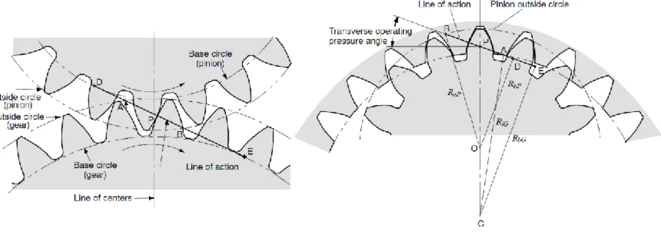
2.8 Spur Gear Background and Nomenclature 29

2.8.1 Internal Gears 31

2.8.2 Spur Gear Basic Geometry 32

2.8.3 Design Methods for Involute Gears 33

2.8.3.2 Working Bending Stress 34 2.8.3.3 Fundamental Contact Stress Formula 34

2.8.3.4 Working Contact Stress 35

Chapter 3 – Engine Modelling 37

3.1 Engine Parametric Review 37

3.1.1 Bore x Stroke 37

3.1.2 Combustion Timings 38

3.2 Initial Parameters 39

3.3 Engine Kinematics 40

3.4 Engine Dynamics 43

3.4.1 Closed Cycle Single-Zone Model 43

3.4.2 Slider Crank Engine Dynamics 45

3.4.3 Geared Hypocycloid Engine Dynamics 47

Chapter 4 – Engine Design 51

4.1 Materials Properties 51

4.1.1 Nitralloy N (AMS 6475) 51

4.1.2 Ferrium S53® (AMS 5922) 52

4.1.3 242.0, 319.0 and A390.0 Aluminium Alloys 53

4.2 Piston and Rod Design 58

4.3 Cylinder Design 62

4.4 Geared Hypocycloid Mechanism Design 65

4.4.1 Geometric Parameters 65

4.4.2 Correction Factors for Bending and Contact Stress 67 4.4.3 Face Width for Pinion and Gear from Bending and Contact Stresses 70

4.5 Crankshaft Design 73

4.6 Output Shaft and Support Shaft Sets Design 75

4.6.1 Balancing 75

4.7 Belt Drive Design 77

4.8 Bearing Selection 77

4.9 Crankcase Design 80

4.10 Final Design 82

Chapter 5 – Results 83

5.1 Engine Performance 83

5.1.1 Opposed Piston Slider Crank Engine 83

5.1.2 Opposed Piston Geared Hypocycloid Engine 87

5.2 Engine Comparison 91

Chapter 6 – Conclusions 95

6.2 Future Work 97

Bibliography 99

List of Figures

Figure 2.1. The four-stroke cycle. From left to right: induction stroke, compression stroke,

expansion stroke, exhaust stroke. ... 6

Figure 2.2. The two-stroke cycle. From left to right: compression stroke, expansion stroke. .. 7

Figure 2.3. Ideal air standard Otto cycle. ... 8

Figure 2.4. Closed system process in a four-stroke engine (left) and p-V changes for a closed system process (right)... 12

Figure 2.5. Definition of flame-development angle (∆𝜃d) and rapid-burning angle (𝜃b) on mass fraction burned versus crank angle curve. ... 13

Figure 2.6. Geometry of slider crank engine. ... 17

Figure 2.7. Example of a p-V diagram for a two-stroke engine (left) and four-stroke engine (right). ... 18

Figure 2.8. Sketch from Wiseman US Patent #6510831. ... 23

Figure 2.9. Hypocycloid concept. ... 25

Figure 2.10. Geometry of geared hypocycloid engine. ... 26

Figure 2.11. Wittig gas engine. ... 27

Figure 2.12. Cross-section through view of Jumo 205. ... 29

Figure 2.13. Generation of an involute (left) and involute action (right). ... 30

Figure 2.14. Meshing between external spur gear (left) and internal spur gear (right) with its pinion. ... 32

Figure 2.15. Basic geometry of a spur gear tooth. ... 33

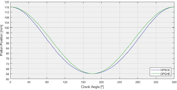
Figure 3.1. Piston position for the OPSCE and OPGHE models during a crank revolution. ... 40

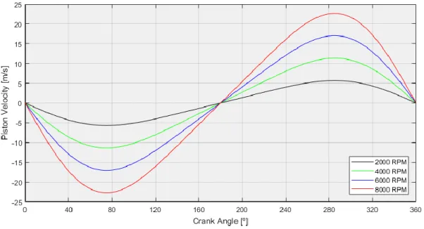
Figure 3.2. Piston velocity for the OPSCE model during a crank revolution. ... 41

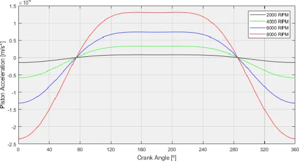
Figure 3.4. Piston acceleration for the OPSCE model during a crank revolution. ... 42

Figure 3.5. Piston acceleration for the OPGHE model during a crank revolution. ... 42

Figure 3.6. Volume chamber for the OPSCE and OPGHE models during a crank revolution. ... 43

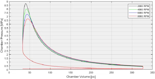
Figure 3.7. Pressure-volume (p-V) diagram for the OPSCE model at various operating speeds. ... 45

Figure 3.8. Forces applied to the piston for the OPSCE model during the cycle at 4000 rpm (top) and 8000 rpm (bottom). ... 46

Figure 3.9. Instantaneous torque output for the OPSCE model during the cycle at various operating speeds. ... 47

Figure 3.10. Pressure-volume diagram (p-V) for the OPGHE model at various operating speeds. ... 47

Figure 3.11. Forces applied to the piston for the OPGHE model during the cycle at 4000 rpm (top) and 8000 rpm (bottom). ... 48

Figure 3.12. Instantaneous torque output for the OPGHE model during the cycle at various operating speeds. ... 49

Figure 3.13. Tangential gear tooth load for the OPGHE model during the cycle at various operating speeds. ... 49

Figure 4.1. Piston and rod geometry. ... 58

Figure 4.2. Two views of the piston design. ... 62

Figure 4.3. Two views of the cylinder design without (left) and with (right) heat fins. ... 64

Figure 4.4. View of the internal gear (left) and pinion (right). ... 72

Figure 4.5. Side crankshaft (left) and centre crankshaft (right). ... 73

Figure 4.6. View of the crankshaft. ... 75

Figure 4.7. View of the output shaft set (top) and support shaft set (bottom). ... 77

Figure 4.8. Sliding (left) and rolling (right) contact bearings. ... 78

Figure 4.9. Render of HK 2516 (top left), 6013 M (top right), 625-2RS1 (bottom left) and HN 1516 (bottom right) SKF bearings. ... 79

Figure 4.10. View of the central crankcase. ... 80

Figure 4.11. View of the front crankcase (top left and bottom) and back crankcase (top right and bottom)... 81

Figure 4.12. Cross-section view of the designed OPGHE. ... 82

Figure 4.13. External view of the designed OPGHE. ... 82

Figure 5.1. Average torque output for the OPSCE model. ... 83

Figure 5.2. Power output for the OPSCE model. ... 84

Figure 5.3. Specific fuel consumption for the OPSCE model. ... 84

Figure 5.4. Mean effective pressure for the OPSCE model. ... 85

Figure 5.5. Fraction of fuel energy loss for the OPSCE model. ... 86

Figure 5.6. Thermal efficiency for the OPSCE model. ... 86

Figure 5.7. Average torque output for the OPGHE model. ... 87

Figure 5.8. Power output for the OPGHE model. ... 87

Figure 5.9. Specific fuel consumption for the OPGHE model. ... 88

Figure 5.10. Mean effective pressure for the OPGHE model. ... 88

Figure 5.11. Fraction of fuel energy loss for the OPGHE model. ... 89

Figure 5.12. Thermal efficiency for the OPGHE model. ... 90

Figure 5.13. Power-to-weight ratio for the OPGHE model. ... 90

Figure 5.14. Average torque output comparison between the OPSCE and OPGHE models. .... 91

Figure 5.15. Power output comparison between the OPSCE and OPGHE models. ... 91

Figure 5.16. Specific fuel consumption comparison the between OPSCE and OPGHE models. 92 Figure 5.17. Mean effective pressure comparison between the OPSCE and OPGHE models. .. 92

Figure 5.18. Fraction of fuel energy loss comparison between the OPSCE and OPGHE models. ... 93

List of Tables

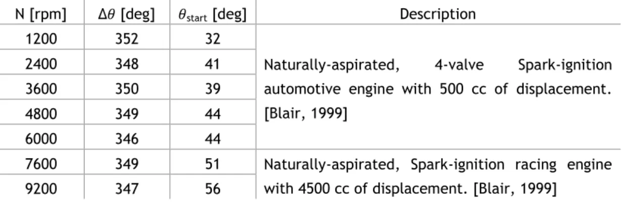
Table 3.1. Combustion data for two engines at different operating speeds. ... 38

Table 3.2. Initial parameters for modelling. ... 39

Table 4.1. Mechanical properties of Nitralloy N. ... 52

Table 4.2. Mechanical properties of Ferrium S53. ... 53

Table 4.3. Mechanical properties of sand-cast 242.0-T571 aluminium alloy. ... 56

Table 4.4. Mechanical properties of sand-cast 319.0-T6 aluminium alloy. ... 56

Table 4.5. Mechanical properties of sand-cast A390.0-T6 aluminium alloy. ... 57

Table 4.6. Dimensions of the piston and rod. ... 61

Table 4.7. Dimensions of the cylinder. ... 64

Table 4.8. Geometry factors interpolated from AGMA 908-B89 tables. ... 66

Table 4.9. Initial geometric parameters for the pinion and gear. ... 67

Table 4.10. Correction factors. ... 70

Table 4.11. Face width for a single gearset considering various addendum modification factors and number of teeth. ... 71

Table 4.12. Face width for a twin gearset considering various addendum modification factors and number of teeth. ... 71

Table 4.13. Dimensions for the geared hypocycloid mechanism. ... 72

Table 4.14. Dimensions of the crankshaft. ... 74

Table 4.15. Mass and distance of centre of mass considering symmetry in reference to the plane intersecting the centre of the crankpin and cylinder axis... 76

Table 4.16. Properties of SKF bearings. ... 79

List of Abbreviations and Symbols

Abbreviation

or Symbol Nomenclature Units

a Acceleration m/s2

ha Addendum mm

x Addendum Modification Factor AFR Air/Fuel Ratio

AFRstoich Air/Fuel Stoichiometric Ratio

β Angle Between Connecting Rod and Axis of the Cylinder º

𝜃start Angle at Start of Combustion º

EVC Angle at Exhaust Valve Close º

EVO Angle at Exhaust Valve Open º

IVC Angle at Intake Valve Close º

IVO Angle at Intake Valve Open º

σFP Allowable Bending Stress MPa

σb Allowable Bending Stress for Crankpin MPa

σHP Allowable Contact Stress MPa

σt Allowable Bending (Tensile) Stress MPa

Creboring Allowance for Reboring mm

σS Allowable Shear Stress MPa

σf Allowable Tensile Strength MPa

σbolt Allowable Tensile Stress for Material of Bolts MPa

N Angular Velocity rpm

𝜔 Angular Velocity rad/s

T

̅q Average Torque N.m

A Area m2

t2 Axial Thickness of Piston Ring mm

j Backlash mm

B Bore m

RBHS Bore/half-stroke Ratio RBS Bore/stroke Ratio BDC Bottom Dead Centre HB Brinell Hardness

c Clearance mm

Vc Clearance Volume m3

ηc Combustion Efficiency

ηcmax Combustion Maximum Efficiency CI Compression Ignition

CR Compression Ratio

aNu Constant for Nusselt Number

aweibe Constant for Weibe Function

mweibe Constant for Weibe Function

Ch Convection Heat Transfer W/(m2.K)

𝜃 Crank Angle º

r Crank Radius m

hd Dedendum mm

ρ Density kg/m3

dbolt Diameter of Bolts mm

dcrankpin Diameter of Crankpin mm

dr Diameter of Piston Rod mm

dshaft Diameter of Output Shaft mm

b Distance m

dBDC Distance Between both pistons at BDC mm

dTDC Distance Between both pistons at TDC mm

dforce Distance Between Centre of Bearing and Force Applied at _Crankshaft mm

dbearing Distance Between Centre of Bearings mm

dcentre Distance Centre mm

Cmf Distribution Factor KV Dynamic Factor mm ∆𝜃 Duration of Combustion º η Efficiency ZE Elastic Coefficient (N/mm2)0.5 E Elastic Modulus Pa FW Face Width mm rt Fillet Radius mm F Force N

Ft Force Applied to the Piston N

Fi Force of Inertia N

Fp Force of Pressure N

4S Four-Stroke

ηfuel Fuel Conversion Efficiency

QHV Fuel Heat Power J/kg

GHE Geared Hypocycloid Engine

bgroove Groove Depth for Piston Ring mm

CH Hardness Ratio Factor

Q Heat J

Cp Heat Capacity at Constant Pressure J/(kg.K)

Cv Heat Capacity at Constant Volume J/(kg.K)

H Heat Flowing Through the Piston Head J

QR Heat Released from Combustion J

QL Heat Lost to Heat J

Qvap Heat Lost to Vaporize Fuel J

Lrod Height of Piston Rod mm

Lpiston Height of Piston Head mm

HPSTC Highest Point of Single Tooth Contact

R Ideal Gas Constant J/(kg.K)

ICE Internal Combustion Engine

IDcap Internal Diameter of Piston Rod Cap mm

U Internal Energy J

Cmc Lead Correction Factor

lcrankpin Length of the Crankpin mm

Lcylinder Length of the Cylinder mm

YN Life Factor ZN Life Factor

Km Load Distribution Factor

m Mass kg

χb Mass Fraction of Fuel Burn

ṁ Mass Flow kg/s

dm Mass Flow Increment kg

ηcmax Maximum Combustion Efficiency

Fbearing Maximum Force Applied at the Main Bearing N

t3 Maximum Thickness of Piston Barrel mm

mep Mean Effective Pressure Pa

S̅p Mean Piston Velocity m/s

Ce Mesh Alignment Correction Factor Cma Mesh Alignment Factor

t4 Minimum Thickness of Piston Barrel mm

M Momentum N.m

mn Normal Module mm

nbolt Number of Bolts nR Number of Revolutions

nrings Number of Rings

Nu Nusselt Number OPE Opposed Piston Engine

OPGHE Opposed Piston Geared Hypocycloid Engine OPSCE Opposed Piston Slider Crank Engine

KO Overload Factor

σc Permissible Hoop Stress MPa

Cpf Pinion Proportion Factor Cpm Pinion Proportion Modifier

apiston Piston Acceleration m/s2

Apiston Piston Area m2

Spiston Piston Position m

vpiston Piston Velocity m/s

dpitch Pitch diameter mm

vt Pitch-line Velocity m/s

I Pitting Resistance Factor ν Poisson’s Ratio

Cheat Portion of Heat Released during Combustion that Flows _{through the Piston Head}

P Power W

p Pressure Pa

Ф Pressure Angle º

pw Pressure of Gas on the Cylinder Wall MPa

t1 Radial Thickness of Piston Ring mm

Cr Radiation Heat Transfer W/(m2K4)

KR Reliability Factor Re Reynolds Number KB Rim Thickness Factor

HR15N Rockwell 15-N Hardness Scale

l Rod Length m

SF Safety Factor SH Safety Factor KS Size Factor

SCE Slider Crank Engine SI Spark Ignition

sfc Specific Fuel Consumption g/kWh

γ Specific Heat Capacity J/(kg.K)

S Stroke m

Cf Surface Condition Factor

Fgt Tangential Gear Tooth Load N

T Temperature K

TC Temperature at Centre of Piston Head K

TE Temperature at Edge of Piston Head K

KT Temperature Factor ηt Thermal Efficiency

t Thickness mm

tcrankweb Thickness of Crankweb mm

tcw Thickness of Cylinder Wall mm

tH Thickness of Piston Head mm

dt Time interval s

J Tooth Bending Geometry Factor TDC Top Dead Centre

Tq Torque N.m

𝜃total Total Cycle Angle º

Av Transmission Accuracy Level Cmt Transverse Load Distribution Factor UHS Ultrahigh-Strength

μ Viscosity kg/(s.m)

V Volume m3

Vdisplaced Volume Displaced by the piston m3

Vdisplacement Volume of Displacement m3

ht Whole Depth mm

WOT Wide-Open-Throttle

w Width mm

b2 Width of Other Lands mm

wcrankweb Width of the Crankweb mm

b1 Width of Top Land mm

W Work J

σF Working Bending Stress MPa

σH Working Contact Stress MPa

Chapter 1

Introduction

Ever since the industrial revolution and the development of the steam engine, a huge technological advance took place. One of the main contributors is the engine, which can be described as a machine that converts chemical energy into mechanical energy [Heywood, 1988] and is essential to our industrialized civilization. In fact, our modern society would not be possible if not for engines in general, but also for aircraft with traffic growing each year at a very fast rate. Powered-flight, as we know it, is only possible not only because of such technological advancements but also because engines evolved to such a degree that the power developed compared to their weight made them suitable for aircraft applications.

Aircraft are not only used for large commercial or military applications with interest in light aircraft increasing, whether it is for tourism, access to remote regions or even as a hobby. Therefore, more focus should be given to the development of one of the most, if not the most, critical component of an aircraft.

1.1 Motivation

With the rising cost of fuel and awareness of emissions, the technology used in conventional engines is approaching its limits. This means an ever-increasing cost of development for engines that meet the increasing rigorous requirements for fuel economy and emissions. Some attention must then be given to alternative configurations and technologies to meet such increasingly strict requirements.

Although some alternative engines and sources of energy exist, these cannot yet meet the requirements for applications in aviation and the cost for development and introduction of such new technologies in the aviation industry is prohibitive. Therefore, some focus must be given to alternative technologies and configurations that can be implemented successfully in a relatively short time with a cost of development and introduction in the aviation industry that can be supported by companies.

1.2 Scope of Work

This thesis focuses on the design of an engine that implements two different technologies in one engine. These are opposed piston configuration in a four-stroke spark-ignition configuration which has not seen much development, contrary to two-stroke diesel engines that have been quite popular in the first half of the 19th _{century and only recently have been given some} attention again [Pirault, 2010]; and a geared hypocycloid mechanism which dates back to when the steam engine was introduced and has been given very little attention, despite its promising advantages over slider crank mechanisms.

1.3 Objectives

This thesis aims to propose an alternative engine configuration to be used in aircraft applications. A comparison between the designed opposed piston geared hypocycloid and slider crank engines is provided to understand the possible performance gains of one over the other. This was done by developing a model in MATLAB to compare both engines. Then, the parts were designed in CATIA V5 and assembled to more easily view the design. The study of heat dissipation via the heat fins, the valve system and consequent intake and exhaust processes are beyond the scope of this study.

1.4 Outline

To provide an easier reading of this work, this thesis was organized in six chapters as will be described next.

This first chapter gives the motivation behind this study. The approach considered is also explained and the objectives presented. Finally, the structure of this thesis is described. The second chapter, designated State of the Art, considers the internal engine background and explains the work and thermodynamic cycles relevant for this study. The appropriate background referring to a more accurate simulation of the cycles is also presented. Next, some engine operating parameters are explained which will be included in the model. Finally, an overview of both slider crank and geared hypocycloid mechanisms is given followed by opposed piston engines and spur gears, both internal and external.

The third chapter focuses on the engine modelling with an initial parametric review of other engines being done as a starting point and to more closely model the combustion timings. It is followed by the definition of the initial parameters for the model ending with the results for the kinematics and dynamics of both engines.

The fourth chapter describes the design process for each component of the engine proposed in this study and shows the respective CATIA parts. Initially, the materials selected are explained and its properties presented with two steel alloys and three aluminium alloys having been selected. Then, the piston and rod design is explained, followed by the cylinder, gearset, crankshaft, output and support shaft where the balancing of the engine is taken into account, ending with considerations for the belt drive, bearings selected and crankcases. At the end, the final design is presented.

The fifth chapter presents the results obtained from the model for the performance of each engine and a comparison is made. The average torque, power, specific fuel consumption, mean effective pressure, fraction of fuel energy loss and thermal efficiency are considered for both engines. The power-to-weight ratio was also considered for the opposed piston considered in this study.

The sixth and final chapter presents the conclusions taken at the end of this study. It also suggests alternative materials that may have an impact on the engine performance as well as possible improvements ending with suggestions for future work.

Chapter 2

State of the Art

2.1 Internal Engine Background

An Internal Combustion Engine (ICE) is an engine where chemical energy is released and converted to mechanical energy through the combustion of a mixture of fuel and oxidizer, usually air. [Heywood, 1988] Contrary to external combustion engines, the combustion in ICE occurs inside the engine and so, the mixture of fuel and air and the burned products are the actual working fluids. The term ‘Internal Combustion Engines’ may be applied to reciprocating ICE or to open circuit gas turbines. However, the term ‘reciprocating’ is usually omitted and when the term ICE is used, it refers to reciprocating internal combustion engines, unless otherwise stated. [Stone, 1999]

There are two main types of ICE - spark ignition (SI) engines where a spark ignites the fuel and compression ignition (CI) engines where the fuel ignites spontaneously due to the rise in temperature and pressure during combustion. Other terms used to refer to SI engines are petrol, gasoline or Otto engines while CI engines may also be referred to as Diesel engines.

2.2 Work Cycle

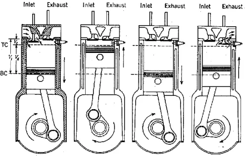
During each crankshaft revolution of an ICE there are two piston strokes, and so there are two main operating cycles in which both engines may be designed to operate – two- or four- stroke. The four-stroke cycle can be described, with reference to figure 2.1, by: [Stone, 1999]

1. The induction stroke. The inlet valve opens, and a charge of air is drawn in as the piston travels down the cylinder. For SI engines, usually fuel pre-mixed with air is drawn in while CI engines only draw in air.

2. The compression stroke. Both the inlet and exhaust valves and the charge is compressed as the piston travels up the cylinder. As the piston approaches top dead centre (TDC), ignition occurs. In SI engines, this usually occurs with a spark while CI engines, fuel is injected instead and auto-ignites.

3. The expansion, power or working stroke. Combustion occurs which raises the pressure and temperature and forces the piston down the cylinder. At the end of this stroke, as the piston approaches bottom dead centre (BDC) the exhaust valve opens.

4. The exhaust stroke. The exhaust valve remains open, the burned gases are expelled as the piston travels up the cylinder, and the exhaust valve is closed at the end of this stroke.

The four-stroke cycle may sometimes be summarized as ‘suck, squeeze, bang and blow’. To provide energy for the other three strokes, some of the power from the expansion stroke is stored in a flywheel. [Stone, 1999]

Figure 2.1. The four-stroke cycle. From left to right: induction stroke, compression stroke, expansion stroke, exhaust stroke. [Heywood, 1988]

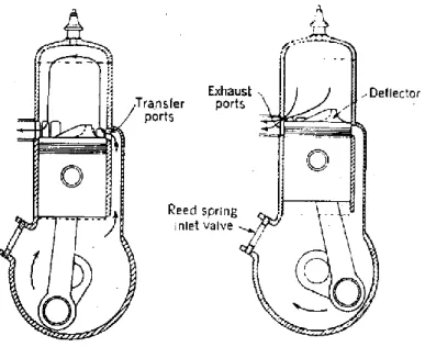
The two-stroke cycle eliminates both the induction and exhaust strokes and can be described, with reference to figure 2.2, by: [Stone, 1999]

1. The compression stroke. Similar to the four-stroke cycle, a charge is compressed as the piston travels up the cylinder. As the piston approaches TDC, ignition occurs. Simultaneously, a charge is drawn in through a spring loaded non-return inlet valve by the underside of the piston.

2. The power stroke. Similar to the four-stroke cycle, combustion occurs which raises the pressure and temperature and forces the piston down the cylinder. Simultaneously, the charge in the crankcase is compressed by the downward motion of the piston. The exhaust port is uncovered and blowdown occurs as the piston approaches the end of its stroke. When at BDC, the piston uncovers the transfer port and the charge compressed in the crankcase expands into the cylinder.

When comparing two- and four-stroke engines of similar sizes operating at a specific speed, the former will produce more power than the latter because it has twice as many power strokes per unit time. However, the two-stroke engine will likely have lower efficiency than the four-stroke engine because ensuring efficient induction and exhaust processes is an issue. This is more evident for SI engines as the pressure inside the crankcase may be below atmospheric pressure at part throttle operation, with a rich air/fuel mixture becoming necessary for all conditions and, therefore, low efficiency. [Stone, 1999]

Figure 2.2. The two-stroke cycle. From left to right: compression stroke, expansion stroke. [Heywood, 1988]

2.3 Thermodynamic Cycle

There are several thermodynamic cycles on which an engine can operate. However, in this study only the Otto Cycle will be considered.

2.3.1 Ideal Otto Cycle

The thermodynamic cycle on which four-stroke SI engines operate is often referred to as the Otto cycle. Theoretically, the ideal Otto cycle assumes for each stroke of the cycle that [Blair, 1999]:

a) The compression stroke begins at BDC and is an isentropic, i.e., adiabatic, process. b) All heat release (combustion) takes place at constant volume at TDC.

c) The expansion stroke begins at TDC and is an isentropic, i.e., adiabatic, process. d) A heat rejection process (exhaust) occurs at constant volume at BDC.

(2.2)

(2.3) (2.1) Both compression and expansion processes are considered to be isentropic and adiabatic (ideal conditions) where the working fluid is air. Those processes can be calculated as: [Blair, 1999]

𝑝𝑉

= 𝑐𝑜𝑛𝑠𝑡𝑎𝑛𝑡

The exponent (γ) is the ratio between heat capacity at constant pressure (Cp) and heat capacity at constant volume (Cv), and assumes a value for air of 1.4, as:

𝛾 =

𝐶

𝐶

The thermal efficiency (ηt) of the cycle is given by:

𝜂

= 1 −

1

𝐶𝑅

where CR is the compression ratio of the engine and will be discussed later. The thermal efficiency may be defined as the ratio between the work produced per cycle and the heat available as input per cycle [Blair, 1999]. It can be observed that the thermal efficiency depends on the compression ratio and not the temperatures in the cycle and with increasing compresson ratio there’s increasing thermal efficiency.

(2.4) (2.5) (2.6) (2.7) (2.8) (2.9)

2.3.1.1 Thermodynamic Navigation around the Ideal Otto Cycle

Referring to figure 2.3, the cycle commences at BDC, at point 1. The mass of air (m1) in the cylinder is then given by: [Blair, 1999]

𝑚

=

𝑝

𝑉

𝑅𝑇

And the mass of air trapped in the cylinder (mair), by:

𝑚

=

𝑝

𝑉

𝑅𝑇

Where Vdisplaced is the volume displaced by the piston and R is the ideal gas constant. The mass of fuel trapped (mfuel) is then found by:

𝑚

=

𝑚

𝐴𝐹𝑅

Where AFR is the air/fuel ratio and will be described later. The heat transfer at TDC is equivalent to the heat energy in the fuel:

𝑄

= 𝜂

𝑚

𝑄𝐻𝑉

Where ηc is the combustion efficiency and QHV is the lower heating value of the fuel.

Process 1-2, Adiabatic and Isentropic Compression [Blair, 1999]

The pressure (p2) and temperature (T2) at the end of compression is given, respectively, by:

𝑝

= 𝑝

(

𝑉

𝑉

)

𝑇

= 𝑇

(

𝑉

𝑉

)

(2.10) (2.11) (2.12) (2.13) (2.14) (2.15) (2.16) (2.17) The work and the change of internal energy done during compression is, respectively, negative and positive, and given by:

𝑊

= −𝑚

𝐶

(𝑇

− 𝑇

)

𝑈

− 𝑈

= 𝑚

𝐶

(𝑇

− 𝑇

)

Process 2-3, Constant Volume Combustion [Blair, 1999]

Applying the first law of thermodynamics to the combustion process:

𝑄

= 𝑈

− 𝑈

+ 𝑊

= 𝑚

𝐶

(𝑇

− 𝑇

) + 0

𝑇

= 𝑇

+

𝑄

𝑚

𝐶

Using the state equation and solving for p3:

𝑝

= 𝑝

𝑉

𝑉

𝑇

𝑇

= 𝑝

𝑇

𝑇

The change of internal energy during the process from 2-3 is given by:

𝑈

− 𝑈

= 𝑄

Process 3-4, Adiabatic and Isentropic Expansion [Blair, 1999]

The pressure (p4) and temperature (T4) at end of expansion, after process 3-4 is given by:

𝑝

= 𝑝

(

𝑉

𝑉

)

= 𝐶𝑅

𝑇

= 𝑇

(

𝑉

𝑉

)

= 𝐶𝑅

(2.18) (2.19)

(2.20) (2.21) The work and the change of internal energy done during expansion is, respectively, positive and negative, and given by:

𝑊

= −𝑚

𝐶

(𝑇

− 𝑇

)

𝑈

− 𝑈

= 𝑚

𝐶

(𝑇

− 𝑇

)

Process 4-1, Cycle completion by constant volume heat rejection [Blair, 1999] From the first law of thermodynamics:

𝑄

= 𝑈

− 𝑈

+ 𝑊

= 𝑚

𝐶

(𝑇

− 𝑇

) + 0

𝑈

− 𝑈

= 𝑄

= 𝑚

𝐶

(𝑇

− 𝑇

)

2.3.1.2 Otto Cycle in a Closed System

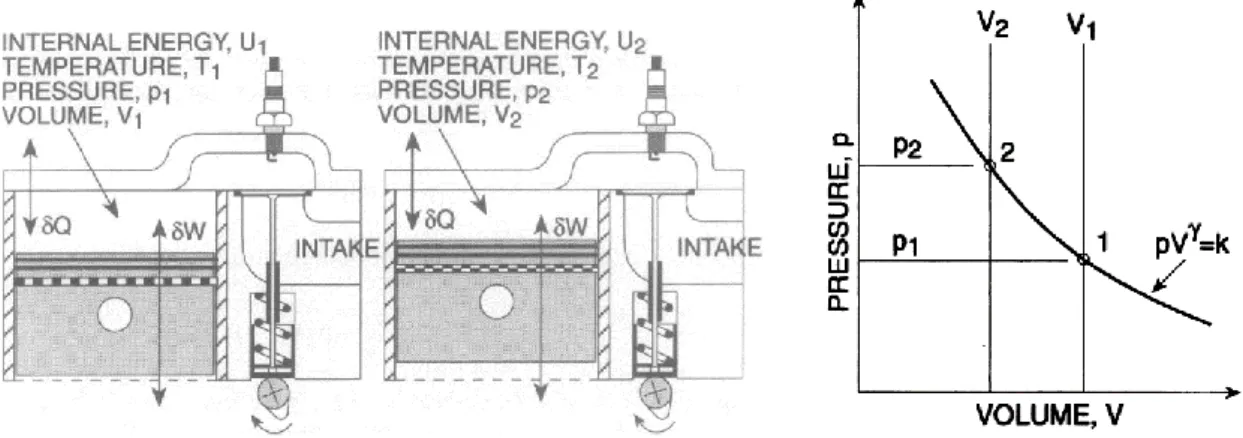
For design purposes, the ideal Otto cycle is quite inaccurate. For this reason, the first step to more accurately predict the operation of the engine is to introduce a combustion process that relates the burning of fuel with respect to time. The next step in view of improving accuracy is introducing heat transfer loss into the simulation of the ideal Otto cycle, making it no longer an ideal cycle though. This heat transfer loss no longer considers the processes to be ideal (isentropic and adiabatic). Finally, another step is to consider friction and pumping losses that occur in the engine cycle. [Blair, 1999] However, this last step will not be included in this model.

The engines were modelled as a closed system, which means that the mass within the system is constant, i.e., the volume, pressure and temperature may change but the mass does not. It also considers all the gas within the cylinder when all valves or apertures to the cylinder are closed and assumes that piston rings make a perfect gas seal with the cylinder walls. A typical situation is illustrated in figure 2.4 where the piston moves from position 1 to position 2 and a compression process occurs, with the volume decreasing from V1 to V2 and the pressure increasing from p1 to p2. For this compression process to occur, the piston must expend work. The data on pressure and volume are graphed in figure 2.4. An expansion process would have occurred if the piston had been descending instead. [Blair, 1999]

(2.22) (2.23) (2.24) (2.25) (2.26)

Figure 2.4 – Closed system process in a four-stroke engine (left) and p-V changes for a closed system process (right). [Adapted from Blair, 1999]

If a gas experiences a work process (δW) within a closed system, it is observed as a change of volume (dV) at pressure (p), and can be evaluated by: [Blair, 1999]

𝛿𝑊 = 𝑝𝑑𝑉

Applying the first law of thermodynamics for a closed system, it is possible to relate any work change (δW) to any change of heat transfer (δQ) and internal energy (dU) as:

𝛿𝑄 = 𝑑𝑈 + 𝛿𝑊

If specific to unit of mass, heat transfer (δq), work (δw) and internal energy (du) may be defined, respectively, as:

𝛿𝑞 =

𝛿𝑄

𝑚

𝑑𝑢 =

𝑑𝑈

𝑚

𝛿𝑤 =

𝛿𝑊

𝑚

(2.27)

(2.28)

(2.29) Eq. 2.24 can then be divided across the mass (m) to obtain a specific formulation for the first law of thermodynamics:

𝛿𝑞 = 𝑑𝑢 + 𝛿𝑤

2.3.3 Heat Release Model

The combustion process may be described thermodynamically as a heat addition process to a closed system. It occurs in a chamber of varying volume, the minimum value of which is the clearance volume, Vc. [Blair, 1999]

In single-zone models, a mass fraction burn curve is usually considered to predict the heat release, and is often referred to as a Weibe function. This function represents the fraction of chemical energy released from the fuel burn as a function of crank angle. It varies with an curve from 0% at the start of the combustion to 100% burned at the end of combustion. This s-curve, as represented in figure 2.5, is described as: [Kuo, 1996]

𝜒

= 1 − 𝑒𝑥𝑝 [−𝑎

(

𝜃 − 𝜃

∆𝜃

)

𝑚𝑤𝑒𝑖𝑏𝑒+1

]

Where 𝜃0 is the angle considered for the start of combustion (about equal to the angle of spark firing), ∆𝜃 is angle for which the combustion occurs and the constants aweibe and mweibe are determined experimentally, with real burn fraction curves having been fitted by the Weibe function with aweibe=5 and mweibe=2 [Kuo, 1996 and Heywood, 1988].

The heat release can then be calculated as: [Blair, 1999]

𝛿𝑄 = 𝜂

(𝜒

− 𝜒

)𝑚

. 𝑄𝐻𝑉

Figure 2.5. Definition of flame-development angle (∆𝜃d) and rapid-burning angle (𝜃b) on mass fraction burned versus crank angle curve. [Adapted from Heywood, 1988]

(2.30) (2.31) (2.32) (2.33) (2.34) (2.35) (2.36)

2.3.4 Heat Transfer Model

One of the indispensable issues in studying ICE is heat transfer because decisive parameters of operation such as temperature and pressure inside the cylinder are influenced by it. There are three heat transfer mechanisms: conduction, convection and radiation [Spitsov, 2013]. The heat transfer included in this model was the Annand model, which is referred as being the most effective and accurate method for calculating heat transfer from the cylinder during the closed cycle for SI engine. [Blair, 1999]

Annand’s heat transfer theory proposes an expression for the Nusselt number (Nu) which leads to a conventional derivation for the convection heat transfer (Ch). Therefore, to relate the Reynolds and Nusselt numbers, Annand recommends the following expression:

𝑁𝑢 = 𝑎

𝑅𝑒

With aNu=0.26 or aNu=0.49 for 2-stroke and 4-stroke engines, respectively. The Reynolds number is calculated by:

𝑅𝑒 =

𝜌

𝑆̅

𝐵

𝜇

Where B is the cylinder bore. The values of density (ρcyl), mean piston velocity (S̅p) and viscosity

(μcyl) can be calculated:

𝜌

=

𝑝

𝑅

𝑇

𝑆

=

2𝑆𝑁

60

𝜇

= 7.457x10

_{+ 4.1547x10}

_{𝑇 − 7.4793x10}

_𝑇

Now, the convection heat transfer (Ch) can be extracted from the Nusselt number:

𝐶

=

𝐶

𝑁𝑢

𝐵

The parameter Ck is the thermal conductivity of the cylinder gas. It may be assumed to be identical with that of air at the instantaneous cylinder temperature (Tcy) and calculated as:

(2.37) (2.38) (2.39) (2.40) (2.41) (2.42) The value of the cylinder wall (Twall) is the average temperature of the cylinder wall, and may be assumed to be 350K. [Stone, 1999]

Annand also considers the radiation heat transfer (Cr) to be:

𝐶

= 4.25x10

₍

𝑇

4

_{− 𝑇}

𝑤𝑎𝑙𝑙4

𝑇

− 𝑇

)

The heat transfer (δQL) can be inferred over a crankshaft angle interval (d𝜃) and a time interval (dt) for the mean value of that transmitted to the total surface area exposed to the cylinder gases, with:

𝑑𝑡 =

𝑑𝜃

360

60

𝑁

𝛿𝑄

= (𝐶

+ 𝐶

)(𝑇

− 𝑇

)𝐴

𝑑𝑡

Where the surface area of the cylinder (Acyl) is:

𝐴

= 𝐴

+ 𝐴

+ 𝐴

It should be noted that opposed piston engines don’t have a cylinder head and, therefore, the heat loss is reduced and thermal efficiency is increased.

2.3.5 Fuel Vaporization Model

During the closed cycle, fuel vaporization occurs. For SI engines, this normally occurs during compression and prior to combustion. With 𝜃vap being the crankshaft interval between IVC and the ignition point, and assuming that fuel vaporization occurs linearly during this interval, the rate at which the fuel vaporizes with respect to crank angle (ṁvap) is given by: [Blair, 1999]

ṁ

=

𝑚

𝜃

Therefore, the loss of heat from the cylinder (δQvap) for any given crankshaft interval (d𝜃) may be calculated by:

(2.43)

(2.44) The model described before is only accurate for mixtures that are stoichiometric or richer. For leaner than stoichiometric mixtures, this model may not be accurate and another model based on CI engines should be applied, which is not covered in this study.

2.4 Engine Operating Parameters

When characterizing engine operation, some basic geometrical relationships and parameters are common and will be described next. To an engine user, the following factors are considered of importance [Heywood, 1988]:

1. The performance of the engine over its operating range;

2. The fuel consumption of the engine within this operating range and the cost of the required fuel;

3. The noise and air pollutant emissions of the engine within this operating range; 4. The engine’s initial cost and its installation;

5. The engine’s reliability and durability, its maintenance requirements, and how these affect engine availability and operating costs.

This study will only consider the performance and efficiency of both engines, though the remaining factors listed above may be equally important.

Engine performance is more precisely defined by the maximum power (or maximum torque) available at each speed within the useful engine operating range; and the range of speed and power over which engine operation is satisfactory. [Heywood, 1988]

2.4.1 Geometrical Properties of Reciprocating Engines

The basic geometry of a reciprocating engine may be defined by the compression ratio (CR), which is the ratio between the maximum and minimum cylinder volume; and the bore/stroke ratio (RBS), which is the ratio between the cylinder bore and piston stroke: [Heywood, 1988]

𝐶𝑅 =

𝑉

+ 𝑉

𝑉

𝑅

=

𝐵

𝑆

For SI engines, these parameters have typical values of RC between 8 and 12 and RBS in the range of 0.8 to 1.2 for small- and medium- sized engines, decreasing to about 0.5 for large slow-speed CI engines. [Heywood, 1988] The mean piston velocity is also an important characteristic and has already been described previously.

(2.45)

(2.46) Figure 2.6. Geometry of slider crank engine. [Adapted from Heywood, 1988]

2.4.2 Brake Torque and Power

Torque may be defined as a force applied through a radius to produce a turning moment. It also can be defined as the tendency of a force to rotate an object around a pivot.

The torque (Tq) produced by an engine is, therefore, defined as:

𝑇𝑞 = 𝐹. 𝑏

Where F is the tangential force applied in relation to the crank radius and b is the distance between the centre of rotation and where the force is applied. Throughout the engine cycle, the torque is constantly varying depending on crank angle therefore, the power being developed is also constantly varying. However, if the torque is averaged for the whole cycle, then the power developed in kW (PkW) can be calculated as:

𝑃

= 2𝜋

𝑁

(2.47)

(2.48) With 𝜔 as the angular velocity in rad/s. It can be converted to horsepower (PHP) by:

𝑃

= 1.34102209 𝑃

It should be noted that torque is a measure of an engine’s ability to do work and power is the rate at which work is done. [Heywood, 1988]

2.4.3 Indicated Work per Cycle

The work transfer of gas in the cylinder to the piston due to the pressure can be calculated with such pressure data. If a diagram of the cylinder pressure and volume throughout the engine cycle is plotted, as in figure 2.7, the area enclosed on the p-V diagram, obtained by integrating around the curve, will give the indicated work per cycle, per cylinder (Wc,i): [Heywood, 1988]

𝑤

= ∮ 𝑝 𝑑𝑉

As far as two-stroke cycle are concerned, Eq. 2.48 becomes simple to apply. However, the addition of inlet and exhaust strokes for the four-stroke cycle introduces some ambiguity and so two definitions of indicated output are commonly used. Gross indicated work per cycle (Wi,cg) is defined to be the work delivered to the piston over the compression and expansion strokes only, while net indicated work per cycle (Wi,cn) is defined to be the work delivered to the piston over the entire four-stroke cycle.

Figure 2.7. Example of a p-V diagram for a two-stroke engine (left) and a four-stroke engine (right). [Adapted from Heywood, 1988]

(2.49)

(2.50)

(2.51) In this study only the gross indicated work per cycle will be considered since indicated quantities are used primarily to identify the impact of the compression, combustion and expansion processes on engine performance. [Heywood, 1988]

The indicated work per cycle and the power per cylinder are related:

𝑃

=

𝑊

𝑁

𝑛

Where nR represents the number of crank revolutions for each power stroke per cylinder and is equal to 2 and 1 for four-stroke and two-stroke cycles, respectively. This power is the indicated power, i.e., the rate of work transfer from the gas within the cylinder to the piston.

2.4.4 Mean Effective Pressure

Although torque is an important parameter to evaluate an engine’s performance, it depends on engine size. Therefore, a more useful relative parameter to measure engine performance is obtained by dividing the work per cycle by the cylinder volume displaced per cycle, in dm3_. This parameter is defined as mean effective pressure (mep) and has units of force per unit area: [Heywood, 1988]

𝑚𝑒𝑝 =

𝑃 𝑛

𝑉

₆₀

𝑁

Or, if expressed in terms of torque:

𝑚𝑒𝑝 =

6.28 𝑛

𝑇𝑞

𝑉

The maximum mean effective pressure of good engine designs is well established and is basically constant over a wide range of engine sizes. Typical values for maximum mep, for naturally aspirated SI engines, are 850 kPa to 1050 kPa at the engine speed for maximum torque. At maximum rated power, bmep values are 10 ro 15 % lower. [Heywood, 1988]

2.4.5 Specific Fuel Consumption and Efficiency

When testing an engine, the fuel consumption is measured as a flow rate-mass per unit time (𝑚̇fuel). However, it is more useful to measure how efficiently an engine is using the fuel supplied to produce work. This parameter is termed specific fuel consumption (sfc), and is the fuel flow rate per unit power output: [Heywood, 1988]

(2.52) (2.53) (2.56) (2.55) (2.54)

𝑠𝑓𝑐 =

ṁ

𝑃

Typical best values of sfc for SI engines are about 75 μg/J=270 g/(kW.h). [Heywood, 1988] However, the specific fuel consumption has units. A dimensionless parameter which relates the desired engine output (work per cycle or power) to the necessary input (fuel flow) would have more fundamental value. Therefore, it is commonly used the ratio of the work produced per cycle to the amount of fuel energy supplied per cycle that can be released in the combustion process, and is a measure of the engine’s efficiency. The fuel energy supplied that can be released by combustion is given by the mass of fuel supplied to the engine per cycle times the heating value of the fuel (QHV) which defines its energy content.

This measure of an engine’s efficiency (termed fuel conversion efficiency ηfuel) is given by:

𝜂

=

𝑊

𝑚

𝑄𝐻𝑉

=

𝑃

𝑚

𝑄𝐻𝑉

=

1

𝑠𝑓𝑐. 𝑄𝐻𝑉

2.4.6 Air/Fuel Ratio

Both the air and fuel mass flow rates (𝑚̇air and 𝑚̇fuel, respectively) are normally measured. The ratio between these flow rates is a useful parameter in defining engine operating conditions:

𝐴𝐹𝑅 =

ṁ

ṁ

Conventional SI engines with gasoline as fuel normally operate with AFR between 12 and 18. The model developed in this study includes the possibility of running lean or rich mixtures and their effect in engine operating conditions. However, as seen before, for lean mixtures fuel vaporization should not be considered unless another model for describing it is adopted. As such, it was described the relative air/fuel ratio (λ) for SI engines, as:

𝜆 =

𝐴𝐹𝑅

𝐴𝐹𝑅

The combustion efficiency (ηc) of a gasoline type fuel can be expressed in terms of relative air/fuel ratio from measured data as: [Blair, 1999]

(2.57)

(2.58) For values of λ between 0.75 and 1.2. The maximum value for ηcmax is typically 0.9 for SI engines using gasoline fuel. It should be noted that Eq. 2.56 maximizes at about 12% lean of stoichiometric. [Blair, 1999]

2.5 Slider Crank Engine

The slider crank internal combustion engine (ICE) drives numerous machines from generators and automobiles to boats and aircraft, being the most used nowadays in developed parts of the world. The slider crank mechanism is mainly used to convert the reciprocating motion of the piston into rotary motion of the output shaft.

Although many technological advancements have been made over the past 100 years as far as ICE are concerned, the fundamental slider crank based mechanism has remained essentially unchanged. Despite its success, this mechanism presents two shortcomings:

1. The angle between the connecting rod and the axis of the cylinder (β) that occurs during an engine operation produces a force on the piston perpendicular to the axis of the cylinder, thus causing piston side load. This piston side load causes friction between the piston and the cylinder wall, with consequent reduced efficiency and additional heat that must be dissipated by the cooling system.

2. Balance is an issue due to the reciprocating motion of the piston and the complex motion of the connecting rod. Furthermore, the piston also describes a non-sinusoidal motion which causes a second order vibration and makes even more difficult to achieve engine balance.

2.5.1 Slider Crank Engine Kinematics

The crank engine kinematics such as instantaneous piston position (Spiston), piston velocity (vpiston) and piston acceleration (apiston) can be described, referring to figure 2.6, as a function depending on crank angle (𝜃) as follows [Heywood, 1988]:

𝑆

(𝜃) = 𝑟 cos(𝜃) + (𝑙

_{− 𝑟}

_sin(𝜃)

₎

Knowing that the instantaneous piston velocity is the derivative of the instantaneous piston position, with 𝜔 as the angular velocity in rad/s:

𝑣

(𝜃) = 𝑆′

(𝜃) = [−𝑟. sin(𝜃) −

𝑟

_{cos(𝜃) sin (𝜃)}

(𝑙

_{− 𝑟}

_sin(𝜃)

₎

] 𝜔

Similarly, the instantaneous piston acceleration (apiston) is the derivative of the instantaneous piston velocity, and it can be described as:

(2.59) (2.60) (2.61) (2.62) (2.63) (2.64) (2.65) (2.66) (2.67)

𝑎

(𝜃) = 𝑣

(𝜃) =

[−𝑟. cos(𝜃) −

𝑟

_cos(𝜃)

(𝑙

_{− 𝑟}

_sin(𝜃)

₎

+

𝑟

sin(𝜃)

(𝑙

_{− 𝑟}

_sin(𝜃)

₎

−

𝑟

cos(𝜃)

sin (𝜃)

(𝑙

_{− 𝑟}

_sin(𝜃)

₎

] 𝜔

Finally, the chamber volume (Vchamber) can be described by:

𝑉

(𝜃) = 𝐴

(𝑙 + 𝑟 − 𝑆(𝜃)) + 𝑉

Where Apiston is the piston crown area. The clearance volume (Vc), which is the combustion chamber volume at TDC, can be calculated by:

𝑉

=

𝑉

𝐶𝑅 − 1

2.5.2 Slider Crank Engine Dynamics

Considering the engine dynamics previously described, some of the ICE dynamics may be described. Knowing that the force applied to the piston (Ft) is the sum of both the force of inertia (Fi) and force of pressure (Fp), it is described by:

𝐹

= 𝐹

+ 𝐹

With:

𝐹

= 𝑚

. 𝑎(𝜃)

𝐹

= 𝑝. 𝐴

Knowing the force that is applied to the piston, the instantaneous torque in respect to the crank angle (Tq(𝜃)) and the average torque over the cycle (𝑇̅q) can be calculated by:

𝑇𝑞(𝜃) =

𝐹

cos (𝛽)

𝑟. sin (𝜃 + 𝛽)

𝑇̅𝑞 =

∑ 𝑇𝑞(𝜃)

𝜃

The angle between the connecting rod and the axis of the cylinder () is given by:

𝛽 = sin

(

𝑟 sin 𝜃

𝑙

)

As described previously, the power developed by the engine is given by Eqs. 2.46 and 2.47 and its efficiency by Eq. 2.53.

2.6 Geared Hypocycloid Engine

The first documented cardan geared mechanism dates back to the 15th _{century, named after} Girolamo Cardano (1501 – 1576). However, such mechanisms may have been studied and developed much earlier, using the geometry of Elementa written by Euclid of Alexandria (325 - 265 BC) [Karhula, 2008].

The first engine to implement this mechanism dates back to 1802 with such engine having been developed and built for water pumping in 1805 by British steam engine manufacturer Matthew Murray. In 1875, the German mechanical engineer and professor Franz Releaux (1829 – 1905) presented the basis of both slider crank and cardan gear mechanisms, and is treated as the originator of the mechanism design. Throughout the 20th _{century, the cardan gear mechanism} has not seen much development and adoption with the slider-crank mechanism being much more popular. Research of particular interest began in the mid 1970’s with the work of Ishida who published a paper focusing on the inertial shaking forces and moments of a geared hypocycloid engine and compared with a slider crank engine. This was followed by another paper published in 1986 where a two-stroke cycle single cylinder reciprocating chainsaw utilizing an internal gear system was studied. Later in 1991, another paper was published which provided a list of proposed benefits and design equations for GHE as well as another version of the basic GHE was introduced, which was called the modified hypocycloid engine. In 1998, a team of researchers from Italy released work on the design and testing of a full crank 1255cc two-stroke hypocycloid engine. In 2001, a patent was filled by Mr. Randal Wiseman in a research effort to give a major focus into the cardan gear mechanism, more specifically, the geared hypocycloid mechanism, depicted in figure 2.8.

One of the most recent comprehensive studies regarding GHE was published by Karhula in 2008, where extensive insight in comparing similar slider crank and cardan gear engines is provided. In 2011, Conner provided work with a focus on the balancing and development of a modified engine provided by Wiseman Technologies Inc. (WTI) and comparing its performance with an unmodified engine. Later in 2014, Ray also published some work continuing the development of the engine provided by WTI. In 2016, Azziz published a paper where an enhanced hypocycloid gear mechanism for internal combustion engine applications was proposed as a replacement for slider crank mechanisms to further improve engine performance.

The increasing awareness of emissions and fuel consumption has increased the interest in alternative engine designs, with GHE being one of the alternatives.

2.6.1 Hypocycloid Concept

The geared hypocycloid engine (GHE) takes advantage of the hypocycloid concept to convert the linear motion of the piston into rotary motion of the output shaft. A hypocycloid, by definition, is the curve traced by a fixed point (A) on the circumference of a small circle of radius Ra that rolls without slipping along the inside of a larger fixed circle or radius Rb, as shown in figure 2.9. [Azziz, 2016]

In the particular case of a circle ratio of 2:1, i.e., the diameter of the inner circle is half the diameter of the outer circle, any point in the inner circle draws a straight-line as it rolls around inside the outer circle. This allows a geared hypocycloid mechanism to be designed with a 2:1 gear ratio to convert the linear motion of the piston into rotary motion. This gives the engine some advantages, such as:

1. The piston will describe a sinusoidal motion which is important for engine balance. 2. Reduced or even non-existent piston side-load which leads to reduced friction and heat

and better efficiency.

3. Piston and rod may be designed without piston skirt or pin wrist which reduces its mass and, therefore, the inertial forces that act upon the piston.

Very few engines have been built. Wiseman claims to have tested and compared two similar engines, one with a slider crank and the other with a geared hypocycloid mechanism and registered an improvement in fuel efficiency of 50.5% while producing the same power output. Conner, however, claims to have seen reduced power output and increased fuel consumption. [Conner, 2011]

(2.70) (2.69) (2.68)

(2.71) Figure 2.9. Hypocycloid concept. [Adapted from Ray, 2014]

2.6.2 Geared Hypocycloid Engine Kinematics

The GHE kinematics such as instantaneous piston position (Spiston), piston velocity (vpiston) and piston acceleration (apiston) can be described, referring to figure 2.10, as a function depending on crank angle (𝜃), as follows [Azziz, 2016]:

𝑆

(𝜃) = 2𝑟 cos(𝜃) + 𝑙

Knowing that the instantaneous piston velocity is the derivative of the instantaneous piston position, with 𝜔 as the angular velocity in rad/s:

𝑣

(𝜃) = 𝑆

𝑝𝑖𝑠𝑡𝑜𝑛

(𝜃) = [−2𝑟 sin(𝜃)]𝜔

Similarly, the instantaneous piston acceleration (apiston) is the derivative of the instantaneous piston velocity, and it can be described as:

𝑎

(𝜃) = 𝑣

𝑝𝑖𝑠𝑡𝑜𝑛

(𝜃) = [−2𝑟 cos(𝜃)]𝜔

Finally, the chamber volume (Vchamber) can be described by:

(2.73)

(2.74) (2.72) Where Apiston is the piston crown area. The clearance volume (Vc), which is the combustion chamber volume at TDC, can be calculated by:

𝑉

=

𝑉

𝐶𝑅 − 1

Figure 2.10. Geometry of geared hypocycloid engine. [Adapted from Heywood, 1988]

2.6.3 Geared Hypocycloid Engine Dynamics

Considering the engine dynamics previously described, some of the GHE dynamics may be described. Similar to ICE, the force applied to the piston (Ft) is the sum of both the force of inertia (Fi) and force of pressure (Fp), and can be calculated by Eqs. 2.63, 2.64 and 2.65. Knowing the force that is applied to the piston, the instantaneous torque in respect to the crank angle (Tq(𝜃)) and the average torque over the cycle (𝑇q) can be calculated by:

𝑇𝑞(𝜃) =

𝐹

cos (𝜃)

𝑟. sin(2𝜃)

𝑇̅𝑞 =

∑ 𝑇𝑞(𝜃)

𝜃

(2.75) The tangential gear tooth load (Fgt) can be calculated by: [Azziz, 2016]

𝐹

= 𝐹

sin(𝜃)

As described previously, the power developed by the engine is given by Eqs. 2.46 and 2.47 and its efficiency by Eq. 2.53.

2.7 Opposed Piston Engine

The first public appearance of an opposed piston engine (OPE) was probably a two-stroke, gas-fuelled by Wittig in Germany in 1878, although in 1874 Gilles de Cologne had already built a single cylinder OPE in which one piston was connected to the crankshaft and the other was a free piston. In opposed piston engines, a pair of pistons operate in a single cylinder, which eliminates the need for cylinder heads. Although the concept of OP is applicable to both two- and four-stroke engines, most OP engines developed operate on two-stroke, CI cycles, probably for simplicity and because they were intended to achieve high thermal efficiency and high-power density. The history of OPE can be divided into three main periods – pre-1900, 1900-1945 and post 1945. [Pirault & Flint, 2010].

The pre-1900 period is characterized by the mention and introduction of many key features of the modern OP engine. The key advantages of OPE in comparison to their competitors during that time were simplicity, balance, absence of the then problematic cylinder head joint, relatively light mechanical loading of the crankshafts due to the possibility of large engines with low bore/stroke ratios (B/S), and the benefit in terms of mixing air with the fuel and turbulence generation because of the opposing retreating motion of the pistons. In this period, OPE greatly improved the efficiency of two-strokes, achieving values close to those of four-stroke engines.