MACHINE LEARNING ALGORITHMS FOR DAMAGE DETECTION IN STRUCTURES UNDER CHANGING NORMAL CONDITIONS

INSTITUTE OF TECHNOLOGY

GRADUATE PROGRAM IN ELECTRICAL ENGINEERING

MACHINE LEARNING ALGORITHMS FOR

DAMAGE DETECTION IN STRUCTURES

UNDER CHANGING NORMAL CONDITIONS

MOISÉS FELIPE MELLO DA SILVA

DM 07/2017

UFPA / ITEC / PPGEE

Guamá University Campus

INSTITUTE OF TECHNOLOGY

GRADUATE PROGRAM IN ELECTRICAL ENGINEERING

MOISÉS FELIPE MELLO DA SILVA

MACHINE LEARNING ALGORITHMS FOR

DAMAGE DETECTION IN STRUCTURES

UNDER CHANGING NORMAL CONDITIONS

DM 07/2017

UFPA / ITEC / PPGEE

Guamá University Campus

INSTITUTE OF TECHNOLOGY

GRADUATE PROGRAM IN ELECTRICAL ENGINEERING

MOISÉS FELIPE MELLO DA SILVA

MACHINE LEARNING ALGORITHMS FOR DAMAGE

DETECTION IN STRUCTURES UNDER CHANGING

NORMAL CONDITIONS

Master dissertation submitted to the Exam-ining Board of the Graduate Program in Electrical Engineering from the Federal Uni-versity of Pará to obtain the Master Degree in Electrical Engineering, Area of Concentra-tion in Applied Computing.

UFPA / ITEC / PPGEE

Guamá University Campus

Silva, Moisés Felipe Mello da,

1994-Machine learning algorithms for damage detection in structures under changing normal conditions / Moisés Felipe Mello da Silva. - 2017.

Orientador: João Crisóstomo Weyl Albuquerque Costa; Coorientador: Claudomiro de Souza de Sales Junior.

Dissertação (Mestrado) Ű Universidade Federal do Pará, Instituto de Tecnologia, Programa de Pós-Graduação em Engenharia Elétrica, Belém, 2017.

1. Inteligência artiĄcial. 2. Reconhecimento de padrões. 3. Engenharia de estruturas Ű modelos matemáticos. I. Título.

INSTITUTO DE TECNOLOGIA

PROGRAMA DE PÓS-GRADUAÇÃO EM ENGENHARIA ELÉTRICA

MACHINE LEARNING ALGORITHMS FOR DAMAGE

DETECTION IN STRUCTURES UNDER CHANGING

NORMAL CONDITIONS

AUTOR:

MOISÉS FELIPE MELLO DA SILVA

DISSERTAÇÃO DE MESTRADO SUBMETIDA À AVALIAÇÃO DA BANCA EXAMI-NADORA APROVADA PELO COLEGIADO DO PROGRAMA DE PÓS-GRADUAÇÃO EM ENGENHARIA ELÉTRICA DA UNIVERSIDADE FEDERAL DO PARÁ, SENDO JULGADA ADEQUADA PARA A OBTENÇÃO DO GRAU DE MESTRE EM ENGE-NHARIA ELÉTRICA NA ÁREA DE COMPUTAÇÃO APLICADA.

APROVADO EM: 31 / 01 / 2017

BANCA EXAMINADORA:

Prof. Dr. João Crisóstomo Weyl Albuquerque Costa

(Orientador - PPGEE/UFPA)

Prof. Dr. Claudomiro de Souza de Sales Junior

(Coorientador - PPGCC/UFPA)

Prof. Dr. Diego Lisboa Cardoso

(Examinador Interno - ITEC/UFPA)

Prof. Dr. Eloi João Faria Figueiredo

(Examinador Externo - ULHT)

VISTO:

Prof. Dr. Evaldo Gonçalves Pelaes

I would like to dedicate this dissertation and my entire life’s work to my mother, Cátia Regina Mello da Silva. She inspired me with superb dedication and gentle care. You’ll be proud of me, wherever you are. I promise you that.

I thank to my father, José Carlos Lima da Silva, for the unconditional support provided me. I live to make you proud.

For my aunt, Lúcia Guerreiro, hugs and kisses. You’re the one who can get close to fill the gap left by mommy. Love you.

To the professor Claudomiro de Souza de Sales Junior who accompany and drive my career since I got in the university, a thank you. Also, thank to professor João Crisós-tomo Weyl Albuquerque Costa for friendship, companionship, experience, guided and knowledge provided in LEA.

In special to my friends Adam Santos, Cindy Fernandes and Reginaldo Santos, whose friendship, I hope, can carry on for the life.

Thanks to my best friend, Thiago Araújo, who is closer than a brother. May our partnership last for life.

And, for you, Luena Canavieira, my dear, nothing that I could say is enough to represent your importance to me. In the absence of words, I prefer the simple ones: thank you, Lulu.

My acknowledgements for the financial support received from CAPES1_{, CNPQ}2

and INESC P&D Brasil3_.

1

http://www.capes.gov.br/

2

http://www.cnpq.br/

3

“You can see a mountain as one of two ways: as an insurmountable barrier or as manner to grow further.” Unknown.

1 Introduction 1

1.1 Context . . . 1

1.2 Related work . . . 3

1.2.1 Traditional approaches for damage detection . . . 4

1.2.2 Cluster-based approaches for damage detection . . . 5

1.3 Justification . . . 6

1.4 Motivation . . . 7

1.5 Objectives . . . 7

1.6 Original contributions . . . 8

1.7 Organization of dissertation . . . 9

2 Statistical pattern recognition for structural health monitoring 10 2.1 Operational evaluation . . . 10

2.2 Data acquisition . . . 11

2.3 Damage-sensitive feature extraction . . . 11

2.4 Statistical modeling for feature classification . . . 12

2.4.1 Linear principal component analysis . . . 13

2.4.2 Auto-associative neural network . . . 14

2.4.3 Kernel principal component analysis . . . 15

2.4.4 Mahalanobis squared-distance . . . 17

2.4.5 Gaussian mixture models . . . 18

3 Proposed machine learning algorithms for data normalization 20 3.1 Deep learning algorithms . . . 20

3.1.1 Autoencoders . . . 21

3.1.2 Stacked autoencoders . . . 22

3.1.3 Deep autoencoders and traditional principal component analysis . 24 3.2 Agglomerative clustering . . . 26

3.2.1 Agglomerative concentric hyperspheres . . . 27

3.2.1.1 Initialization procedures . . . 29

4 Experimental results and analysis 31 4.1 Test bed structures and data sets . . . 31

4.1.1 Z-24 Bridge data sets . . . 31

4.1.2 Tamar Bridge data sets . . . 34

4.3.1 PCA-based approaches . . . 37

4.3.2 Comparative study of the initialization procedures . . . 38

4.3.3 Cluster-based approaches . . . 40

4.4 Damage detection with daily data set from the Tamar Bridge . . . 43

4.4.1 PCA-based approaches . . . 43

4.4.2 Cluster-based approaches . . . 44

4.5 Overall analysis . . . 46

5 Conclusions, future research and published works 48 5.1 Main conclusions . . . 48

5.2 Future research topics . . . 49

5.3 Published works . . . 50

Bibliography 52

A Theoretical properties 59

Figure 1 Flowchart of SPR paradigm for SHM (FIGUEIREDO, 2010). . . 10 Figure 2 Schematic representation of an AANN (SOHN; WORDEN; FARRAR,

2002). . . 15 Figure 3 The basic idea behind KPCA (SCHOLKOPF; SMOLA; MULLER, 1998). 16 Figure 4 Comparison between MSD (left) and GMM (right) models (FIGUEIREDO

et al., 2014a). . . 18

Figure 5 General scheme of a simple autoencoder (GOODFELLOW; BENGIO; COURVILLE, 2016). . . 21 Figure 6 Unsupervised layer-wise pre-training and fine adjustment of a nine-layer

deep architecture. . . 23 Figure 7 Flow chart of agglomerative hierarchical clustering. . . 26 Figure 8 ACH algorithm using linear inflation running in a three-component

scenario. . . 28

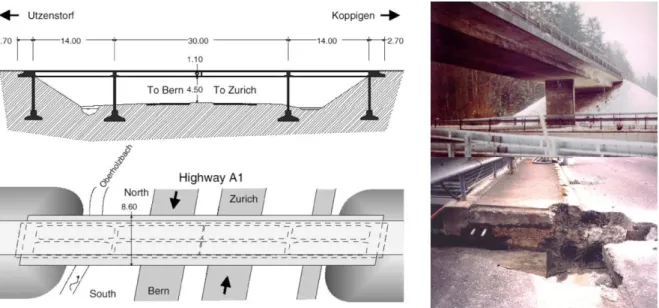
Figure 9 Z-24 Bridge scheme (left) and picture (top right), as well as a damage scenario introduced by anchor head failure (bottom right). . . 32 Figure 10 First four natural frequencies of Z-24 Bridge. The observations in the

in-terval 1-3470 are the baseline/undamaged condition (BC) and observa-tions 3471-3932 are related to damaged condition (DC) (FIGUEIREDO et al., 2014b). . . 33 Figure 11 The Tamar Suspension Bridge viewed from cantilever (left) and River

Tamar margin (right). . . 34 Figure 12 First five natural frequencies obtained in the Tamar Bridge. The

obser-vations in the interval 1–363 are used in the statistical modeling while observation 364-602 are used only in the test phase (FIGUEIREDO et al., 2012). . . 35 Figure 13 Damage indicators along with a threshold defined over the training data

for Z-24 Bridge: (a) DSA-, (b) PCA-, (c) AANN- and (d) KPCA-based approaches. . . 38 Figure 14 ACH damage indicators for different initialization procedures along

with a threshold defined over the training data: (a) random-, (b) uniform-, and (c) divisive-based initialization procedures. . . 40 Figure 15 Damage indicators along with a threshold defined over the training data

the amplitude of the damage indicators for ACH- (a) and GMM-based (b) approaches. . . 42 Figure 17 Damage indicators along with a threshold defined over the training data

for Tamar Bridge: (a) DSA-, (b) PCA-, (c) AANN, and (d) KPCA-based approaches. . . 44 Figure 18 Damage indicators along with a threshold defined over the training data

Table 1 Comparison of the different PCA-based approaches. . . 24

Table 2 Structural damage scenarios introduced progressively (details in (FIGUEIREDO et al., 2014a)). . . 33 Table 3 Number and percentage of Type I/II errors for PCA-based approaches

using the hourly data set from the Z-24 Bridge. . . 37 Table 4 Number of clusters and percentage of Type I and Type II errors for each

ACH initialization procedure using the hourly data set from the Z-24 Bridge. . . 39 Table 5 Number of clusters and percentage of Type I/II errors for cluster-based

approaches using the hourly data set from the Z-24 Bridge. . . 40 Table 6 Number and percentage of Type I errors for PCA-based approaches

using the daily data set from the Tamar Bridge. . . 43 Table 7 Number of clusters and percentage of Type I errors for cluster-based

AANN Auto-Associative Neural Network

ACH Agglomerative Concentric Hypersphere

AIC Akaike Information Criterion

BC Baseline Condition

BIC Bayesian Information Criterion

DC Damage Condition

DI Damage Indicator

DSA Deep Stacked Autoencoder

EM Expectation-Maximization

FA Factor Analysis

GK Gustafson-Kessel

GMM Gaussian Mixture Model

KPCA Kernel Principal Component Analysis

LogL Log Likelihood

ML Maximum Likelihood

MSD Mahalanobis-Squared Distance

NLPCA Nonlinear Principal Component Analysis

PCA Principal Component Analysis

RBF Radial Basis Function

SHM Structural Health Monitoring

SMS Structural Management System

SPR Statistical Pattern Recognition

Engineering structures have played an important role into societies across the years. A suitable management of such structures requires automated structural health monitoring (SHM) approaches to derive the actual condition of the system. Unfortunately, normal variations in structure dynamics, caused by operational and environmental conditions, can mask the existence of damage. In SHM, data nor-malization is referred as the process of Ąltering normal effects to provide a proper evaluation of structural health condition. In this context, the approaches based on principal component analysis and clustering have been successfully employed to model the normal condition, even when severe effects of varying factors impose dif-Ąculties to the damage detection. However, these traditional approaches imposes serious limitations to deployment in real-world monitoring campaigns, mainly due to the constraints related to data distribution and model parameters, as well as data normalization problems. This work aims to apply deep neural networks and propose a novel agglomerative cluster-based approach for data normalization and damage detection in an effort to overcome the limitations imposed by traditional methods. Regarding deep networks, the employment of new training algorithms provide models with high generalization capabilities, able to learn, at same time, linear and nonlinear inĆuences. On the other hand, the novel cluster-based approach does not require any input parameter, as well as none data distribution assumptions are made, allowing its enforcement on a wide range of applications. The superior-ity of the proposed approaches over state-of-the-art ones is attested on standard data sets from monitoring systems installed on two bridges: the Z-24 Bridge and the Tamar Bridge. Both techniques revealed to have better data normalization and classiĄcation performance than the alternative ones in terms of false-positive and false-negative indications of damage, suggesting their applicability for real-world structural health monitoring scenarios.

Estruturas de engenharia têm desempenhado um papel importante para o desenvolvimento das sociedades no decorrer dos anos. A adequada gerência e manutenção de tais estruturas requer abordagens automatizadas para o monitora-mento de integridade estrutural (SHM) no intuito de analisar a real condição dessas estruturas. Infelizmente, variações normais na dinâmica estrutural, causadas por efeitos operacionais e ambientais, podem ocultar a existência de um dano. Em SHM, normalização de dados é frequentemente referido como o processo de Ąltragem dos efeitos normais com objetivo de permitir uma avaliação adequada da integridade es-trutural. Neste contexto, as abordagens baseadas em análise de componentes prin-cipais e agrupamento de dados têm sido empregadas com sucesso na modelagem dessas condições variadas, ainda que efeitos normais severos imponham alto grau de diĄculdade para a detecção de danos. Contudo, essas abordagens tradicionais possuem limitações sérias quanto ao seu emprego em campanhas reais de moni-toramento, principalmente devido as restrições existentes quanto a distribuição dos dados e a deĄnição de parâmetros, bem como os diversos problemas relacionados a normalização dos efeitos normais. Este trabalho objetiva aplicar redes neurais de aprendizado profundo e propor um novo método de agrupamento aglomerativo para a normalização de dados e detecção de danos com o objetivo de superar as limitações impostas pelos métodos tradicionais. No contexto das redes neurais profundas, o em-prego de novos métodos de treinamento permite alcançar modelos com maior poder de generalização. Em contrapartida, o novo algoritmo de agrupamento não requer qualquer parâmetro de entrada e não realiza asserções quanto a distribuição dos dados, permitindo um amplo dominínio de aplicações. A superioridade das abor-dagens propostas sobre as disponíveis na literatura é atestada utilizando conjuntos de dados oriundos de dois sistemas de monitoramento instalados em duas pontes distintas: a ponte Z-24 e a ponte Tamar. Ambas as técnicas revelaram um melhor de-sempenho de normalização dos dados e classiĄcação do que os métodos tradicionais, em termos de falsas-positivas e falsas-negativas indicações de dano, o que sugere a aplicabilidade dos métodos em cenários reais de monitoramento de integridade estrutural.

1 Introduction

1.1

Context

Improved and more continuous condition assessment of civil structures has been demanded by our society to better face the challenges presented by aging civil infrastruc-ture. Structural management systems (SMSs) plan to cover all activities performed during the service life of engineering structures, considering public safety, authorities’ budgetary constraints, and transport network functionality. They possess mechanisms to ensure the structures are regularly inspected, evaluated, and maintained in a proper manner. Hence, a SMS is developed to analyze engineering and economic factors and to attend the author-ities in determining how and when to make decisions regarding maintenance, repair, and rehabilitation of structures (FARRAR; WORDEN, 2013; FIGUEIREDO; MOLDOVAN; MARQUES, 2013).

However, the SMSs still depend on structural inspections, especially on the qual-itative and not necessarily consistent visual inspections, which may impact the struc-tural evaluation and, consequently, the maintenance decisions as well as the avoidance of structural collapses (WENZEL, 2009). In the last years, the structural health monitoring (SHM) discipline has emerged to aid the structural management with more reliable and quantitative information. Although the SMS has already been accepted by the structural managers around the world (CATBAS; GOKCE; GUL, 2012; WORDEN et al., 2015; HU et al., 2016), even though with inherent limitations imposed by the visual inspections, the SHM is becoming increasingly attractive due to its potential ability to detect damage at varying stages and near real-time, with the consequent life-safety and economical benefits (WORDEN et al., 2007; FARRAR; WORDEN, 2013).

The process involves the observation of a structural system over time using pe-riodically sampled response measurements from an array of sensors, the extraction of damage-sensitive features from these measurements, and the statistical analysis of these features to discriminate the actual structural condition for short or long-time periods. Then, once the normal condition has been successfully learned, the model can be used for rapid condition assessment to provide, in nearly real time, reliable information regarding the integrity of the structure.

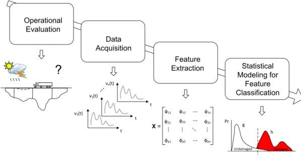
recognition (SPR) problem. Thus, the SPR paradigm for the development of SHM so-lutions can be described as a four-phase process (FARRAR; DOEBLING; NIX, 2001): (1) operational evaluation, (2) data acquisition, (3) feature extraction, and (4) statistical modeling for feature classification.

Particularly, in the feature extraction phase, damage-sensitive features (e.g., nat-ural frequencies, autorregresive model parameters) are derived from the raw data, being correlated with the severity of damage present in the monitored structure. Data com-pression is also an inherent part of most feature extraction procedures. Unfortunately, operational and environmental variations (e.g. temperature, operational loading, humid-ity and wind speed) often arise as undesired effects in the damage-sensitive features and usually mask changes caused by damage, which might negatively influence the proper identification of damage (SOHN, 2007).

In that regard, data normalization procedures are required to surpass the effects of operational and environmental variability, as an effort to improve the damage assessment (CATBAS; GOKCE; GUL, 2012). This procedure is fully connected to the data acqui-sition, feature extraction, and statistical modeling phases of the SHM process, including a wide range of steps for mitigating (or even removing) the effects of normal variations on the extracted features as well as for separating changes in damage-sensitive features caused by damage from those caused by varying operational and environmental conditions (SOHN; WORDEN; FARRAR, 2002; KULLAA, 2011). Without such data normalization procedures, varying operational and environmental conditions will produce false-positive indications of damage and quickly erode confidence in the SHM system. In general, the treatment of such influences starts in data collection (by choosing less sensitive physical parameters to varying normal condition), appears in feature extraction (by selection of features with high sensitivity to damage and insensitive to normal variations), and fin-ishes in the statistical modeling (remaining effects are accounted by automated procedures inspired in machine learning field) (FARRAR; SOHN; WORDEN, 2001).

The most traditional unsupervised approaches used in SHM field are, no doubt, the ones based on Mahalanobis squared distance (MSD) and principal component anal-ysis (PCA) (WORDEN; MANSON; FIELLER, 2000; MALHI; GAO, 2004; YAN et al., 2005c; PURARJOMANDLANGRUDI; GHAPANCHI; ESMALIFALAK, 2014; XIANG; ZHONG; GAO, 2015). They are linear algorithms adapted to act as data normalization and damage detection techniques used to model, mainly, effects of linear variations. How-ever, the linear behavior imposed for these techniques has limited their applicability in SHM. If nonlinearities are present in the monitoring data, the MSD and PCA might fail in modeling the normal condition of a structure because the former assumes the baseline data follow a multivariate Gaussian distribution (or only one data cluster) and the princi-pal components in the latter are independent only if the baseline data is jointly normally distributed.

To extend the capabilities of the traditional methods, improved approaches based on the auto-associative neural network (AANN), kernel PCA and Gaussian mixture mod-els (GMMs) were proposed to deal with real-world structures and more complex SHM applications such that the nonlinear influences on the damage-sensitive features could be accounted for (HSU; LOH, 2010; MALHI; YAN; GAO, 2011; SHAO et al., ; REYN-DERS; WURSTEN; ROECK, 2014; SANTOS et al., 2015; FIGUEIREDO; CROSS, 2013). However, the required input parameters, as well as the usual constraints related to data distribution, make these approaches hard to employ in real-world monitoring campaigns. In some cases, despite of their model complexity and high computational cost, the training procedures do not guarantees a proper modeling of normal conditions, resulting in poor damage detection performance.

1.2

Related work

1.2.1 Traditional approaches for damage detection

Principal component analysis is a common method to perform data normaliza-tion and feature classificanormaliza-tion without directly measure the sources of variability. Yan et al. (YAN et al., 2005a) present a PCA-based approach to model linear environmental and operational influences using only undamaged feature vectors. The number of principal components of the vibration features is implicitly assumed to correspond to the number of independent factors related to the normal variations. A further extension of the proposed method is presented in (YAN et al., 2005b). In this case, a local extension of PCA is used to learn nonlinear relationships by applying a local piecewise PCA in a few regions of the feature space. Although both approaches demonstrate adequate damage detection perfor-mance, the use of PCA imposes serious limitations in the employment of the proposed approaches, such as: only linear transformations can be performed through the orthogonal components; as larger the variance of the component, the greater its importance (in some cases this assumption is untrue); and scale variant (SHLENS, 2002).

To overcome the PCA limitations and detect damage in structures under chang-ing environmental and operational conditions, an output-only vibration-based damage detection approach was proposed by Deraemaeker et al. (DERAEMAEKER et al., 2008). Two types of feature extraction based on automated stochastic subspace identification and Fourier transform are used as damage sensitive-features, as well as the environmental effects and the damage detection are carried out by factor analysis (FA) and a statisti-cal process control, respectively. The results demonstrate that when FA is applied to deal with normal variations both type of features provide reliable damage classification results. However, this approach has been tested only using a numerical model of bridge, which does not ensure its performance in real monitoring scenarios. Furthermore, the FA is also able to learn linear influences as linear PCA.

on the type of features extracted.

The aforementioned drawbacks lead the research efforts to kernel-based machine learning algorithms, which have been widely used in structure monitoring. The ones based on support vector machines (SVM) have demonstrated high reliability and sensitivity to damage. A supervised SVM method to detect damage in structures with a limited number of sensors was proposed in (MITA; HAGIWARA, 2003). Khoa et al. (KHOA et al., 2014) proposed an unsupervised adaptation to dimensionality reduction and damage detection in bridges. Santos et al. (SANTOS et al., 2016b) carried out a comparison study on kernel-based methods. The results demonstrated that those SVM-based approaches has been outperformed by kernel PCA (KPCA), in terms of removing environmental and operational effects and classification performance.

The KPCA is an alternative approach to perform NLPCA. The kernel-trick allows to mapping the feature vectors to high dimensional spaces, which provides nonlinear strengths to linear PCA. Cheng et al. (CHENG et al., 2015) applied KPCA to detect damage on concrete dams subjected to normal variations. Similarly, novelty detection methods were proposed in (OH; SOHN; BAE, 2009; YUQING et al., 2015) by applying KPCA as a data normalization procedure. In these approaches, the problems related to the choice of suitable damage index and estimation of some parameters are addressed. However, the issues related to the choice of an optimal kernel bandwidth and the number of retained components were not fully addressed. Reynders et al. (REYNDERS; WURSTEN; ROECK, 2014) developed an alternative approach to detect damage and eliminate the environmental and operational influences in terms of retained components, and presents a complete scheme to assess the previous issues. However, this approach is not able to completely remove the normal effects, as it deals with a fraction of the environmental and operational effects.

1.2.2 Cluster-based approaches for damage detection

A two-step damage detection strategy based on GMMs has been developed in (FIGUEIREDO; CROSS, 2013; FIGUEIREDO et al., 2014b; SANTOS et al., 2016a) and applied to long-term monitoring of bridges. In the first step, the GMM-based ap-proach models the main clusters that correspond to the normal and stable set of un-damaged conditions, even when normal variations affect the structural response. To learn the parameters of GMMs, the classical maximum likelihood (ML) estimation based on the expectation-maximization (EM) algorithm is adopted in (FIGUEIREDO; CROSS, 2013). This approach applies an expectation step and a maximization step until the log-likelihood converges to a local optimum. Thus, the convergence to the global optimum is not guaranteed.

To overcome the limitations imposed by EM, in (FIGUEIREDO et al., 2014b) the parameter estimation is carried out using a Bayesian approach based on a Markov-chain Monte Carlo method. In (SANTOS et al., 2016a), a genetic-based approach is employed to drive the EM searching towards the global optimum. In these approaches, as the parameters have been learned, a second step is performed to detect damage on the basis of a MSD outlier formation considering the chosen main groups of clusters. The problems concerning these algorithms is related to the number of required parameters to be tuned, as well as their parametric behavior.

Silva et al. (SILVA et al., 2008) proposed a fuzzy clustering approach to detect damage in an unsupervised manner. The principal component analysis and auto-regressive moving average methods are used to data reduction and feature extraction purposes. The normal condition is modeled by two different fuzzy clustering algorithms, the fuzzy c-means clustering and the Gustafson-Kessel (GK) algorithms. The results demonstrated that the GK algorithm outperforms the alternative approach and reveals a better gener-alization performance. However, the damage severity is not properly assessed and both approaches output a significant number of false-negative indications of damage.

1.3

Justification

and knowledge of the structure’s dynamic to decide which method is the most suitable one to each kind of application.

1.4

Motivation

Currently, one of the biggest challenges for transition of SHM technology from research to practice refers to the separation of changes in the feature amplitude caused by damage from those caused by changing operational and environmental conditions. Ac-tually, there are two main approaches to separate those changes. The first implies the direct measure of the sources of variability (e.g., live loads, temperature, wind speed, and/or moisture levels), as well as the structural time-response at different locations of the structure. This input-output approach learns the structural conditions by establishing a direct relation between the normal variations and the actual structural condition. How-ever, such parameterized modeling is hard and complex to deploy in real situations due to the complexity to discover and capture all sources of variability, which still not completely understood (REYNDERS; WURSTEN; ROECK, 2014). The second approach, and the one used in this dissertation, attempts to establish the existence of damage for cases when measurements of the operational and environmental factors that influence the structure’s dynamic response are not available or can not be obtained. Thus, the main purpose is to eschew the measure of operational and environmental variations and physics-based mod-els such as finite element analysis. The present work is motivated by the need of robust unsupervised methods to identify damages in structures subjected to linear/nonlinear variations using only the time-response data from undamaged condition.

1.5

Objectives

The main objectives of this work is to review, develop, and apply several machine learning algorithms to data normalization purposes in the context of the SPR paradigm, capable to detect damage on structures under unmeasured operational and environmental factors. Furthermore, the focus of this work is on the implementation of algorithms that analyze and learn the distributions of the extracted damage-sensitive features from the raw data, in an effort to determine the structural health condition. To achieve these goals, the particular objectives are listed below:

2. Enhance the literature of SHM concerned to damage assessment and identification by comparing the proposed methods with traditional ones.

3. Apply the proposed methods on data sets from real-world structures subjected to rigorous linear/nonlinear effects, as a means of testing their performance and estab-lish comparisons.

Note that even though these procedures might be applied to infrastructure of arbitrary complexity (such as mechanical, aeronautical and naval structures), in this case the procedures are specially posed in the context of bridge applications.

1.6

Original contributions

Many research works have been proposed to improve the damage detection and identification. However, some issues still not completely addressed and treated. In that regard, the main original contributions of this work are the following:

1. Fulfil the gap in literature for robust methods able to remove linear/nonlinear vari-ations for damage detection purposes by proposing two non-parametric algorithms based on deep neural networks and agglomerative clustering, highlighting the fact that the cluster-based method was the one totally designed by the author.

2. The deep neural network can be faced as the first application of deep stacked au-toencoders (DSA) as a data normalization procedure in the context of SHM, which it is intended to overcome the limitations related to the traditional PCA-based approaches.

3. The novel agglomerative concentric hypersphere (ACH) algorithm aims to model the normal conditions of a structure by clustering similar observations related to the same structural state at a given period of time. This straightforward method does not require any input parameter, except the training data matrix, as well as none assumptions related to data distribution are made.

4. Two deterministic initialization procedures rooted on eigenvectors/eigenvalues de-composition and an uniform data sampling are presented. Furthermore, a random initialization is also introduced. These mechanisms are intended to support the ini-tial guess for the clustering procedure.

The results indicate that the proposed approaches has overcome the traditional ones in terms of damage classification and robustness to deal with nonlinear effects caused by normal variations. Furthermore, the proposed cluster-based algorithm demonstrates to be capable to provide physical interpretations about structural conditions, allowing a better understanding of operational and environmental sources of variability.

1.7

Organization of dissertation

2 Statistical pattern recognition for

struc-tural health monitoring

The SHM research community agree that all approaches to SHM can be seen in the context of a pattern recognition problem, which aims to provide not only rea-sonable answers for all possible inputs, but also infer explanation and formalization of the relationships deriving that answers. Thus, the SPR paradigm for the development of SHM applications is usually described as a four phase process, as illustrated in Figure 1 (FIGUEIREDO, 2010; FARRAR; WORDEN, 2013). These phases are briefly described below, giving more attention to the fourth phase, which is the main focus of this work.

?

ν1(t) ν2(t)

νn(t)

...

X =

φ11 φ21

φ12

φ22 φ2n φ1n

φpn φp1 φp2

... ...

... ... ... ... ...

Figure 1 – Flowchart of SPR paradigm for SHM (FIGUEIREDO, 2010).

2.1

Operational evaluation

The main goal of operational evaluation phase it provide answers to four questions regarding the implementation of a monitoring system:

1. What is the life-safety and/or economic justification for performing the structural health monitoring?

3. What are the conditions, both operational and environmental, under which the system to be monitored functions?

4. What are the limitations on acquiring data in the operational environment?

In that regard, operational evaluation seeks to set the boundaries and limitations on the kind of monitored parameters, aiming to determine how the monitoring will be ac-complished. It enables to reduce time and cost efforts during posterior phases, allowing to determine the appropriate features to be extracted from the system being monitored and attempts to exploit unique features of the damage that is to be detected. Otherwise, later phases would be carried out without any reliability in the monitoring system designed.

2.2

Data acquisition

The data acquisition portion of the SHM process involves selecting the exci-tation methods, the sensor types, number and locations, as well as the data acquisi-tion/storage/transmittal hardware. This portion of the process will be application-specific. Economic factors play the major role during acquisition of the hardware to be used for the SHM system. The sensor sensitivity to low level excitation, the data interrogation procedures, as well as the interval at which data should collected are other issues that must be addressed. For example, in applications where life-safety is a critical effort, such as earthquake monitoring, it may be prudent to collect data immediately before and at periodic intervals after a large event. On the other hand, if identify slightly changes in stiffness and geometric properties is the main concern, then it may be necessary to collect data almost continuously at relatively short time intervals once some critical crack has been identified. The kind of strategy is highly dependent of the questions addressed dur-ing operational evaluation. All these contents can affect more or less directly the readdur-ings collected, regarding the presence and location of damage.

2.3

Damage-sensitive feature extraction

type of feature differs from the kind of structure and the objective of monitoring. Fun-damentally, the feature extraction process is based on fitting some model, either physics-or data-based, to the measured response data. The parameters of these models, physics-or the predictive errors associated with them, become the damage-sensitive features. Generally, a degree of signal processing is required in order to extract effective features.

2.4

Statistical modeling for feature classification

Undoubtedly, the portion of the SHM process with least attention in the tech-nical literature is concerned to the development of statistical models for discrimination between features from the undamaged and damaged structures. Statistical modeling for feature classification is concerned with the implementation of algorithms that analyze the distributions of the extracted features in an effort to determine the structural condition at a given period of time. The functional relationship between the selected features and the damage state of the structure is often difficult to define based on physics-based engineering analysis procedures. Therefore, the statistical models are derived using machine learning techniques. These algorithms usually fall into three categories: (i) group classification, (ii) regression analysis, and (iii) outlier or novelty detection. The appropriate algorithm to use depends on the ability to perform supervised or unsupervised learning. In the context of SHM applications, supervised learning is referred to the case where examples of data from damaged and undamaged conditions are available; group classification and regression analysis are often used for this purpose. On the other hand, unsupervised learning arises when only data from the undamaged structure are available for training, where outlier or novelty detection methods are the primary class of algorithms used in this situation. However, for high capital expenditure infrastructures, such as civil ones, the unsupervised learning are often required because only data from the undamaged condition are available.

In SHM, for general purposes, the training matrix X ∈ R𝑛×𝑚 is composed of

𝑛 observations under operational and environmental variability when the structure is

2.4.1 Linear principal component analysis

An output-only technique that has been applied for eliminating environmental influences on features is linear principal component analysis. This multivariate statistical procedure aims to estimate a linear static relationship between the extracted features and the unknown normal influences by reducing the dimensionality of the original input data through a linear projection onto a lower dimensional space. This linear map allows one to remove the normal variations in terms of retained components. In the SHM field, PCA has been used for several purposes (feature selection, feature cleansing and visualization). Herein, PCA is used as a data normalization method.

Assuming the training data matrix X decomposed in the form of (JOLLIFFE,

2002)

X=TU𝑇 = 𝑚

∑︁

𝑖=1

t𝑖u𝑇𝑖 , (2.1)

where T is called the scores matrix and U is a set of 𝑚 orthogonal vectors, u_𝑖, also

called the loadings matrix. The orthogonal vectors can be obtained by decomposing the covariance matrix ofXin the form of Σ = UΛU𝑇, where Λ is a diagonal matrix containing

the ranked eigenvaluesÚ𝑖, andUis the matrix containing the corresponding eigenvectors.

The eigenvectors associated with the higher eigenvalues are the principal components of the data matrix and they correspond to the dimensions that have the largest variability in the data. Basically, this method permits one to perform an orthogonal transformation by retaining only the principal components 𝑑 (⊘𝑚), also know as the number of factors.

Precisely, choosing only the first𝑑 eigenvectors, the final matrix can be rewritten without

significant loss of information in the form of

X=T_𝑑U𝑇_𝑑 +E= 𝑑

∑︁

𝑖=1

t_𝑖u𝑇_𝑖 +E, (2.2)

where E is the residual matrix resulting by the 𝑑 factors. The coefficients of the linear

transformation are such that if the feature transformation is applied to the data set and then reversed, there will be a negligible difference between the original and reconstructed data.

In the context of data normalization, the PCA algorithm can be summarized as follows: the loadings matrix is obtained from X, the test matrix Z is mapped onto the

feature space R𝑑 and reversed back to the original space R𝑚, the residual matrix E is

computed as the difference between the original and the reconstructed test matrix

and finally in order to establish a quantitative measure of damage, the structural health condition is discriminated by generating a damage indicator (DI) and classifying through a threshold. For the 𝑙 feature vector (𝑙 = 1,2, ..., 𝑣), a DI is adopted in the form of the

squared root of the sum-of-square errors (Euclidean norm):

DI(𝑙) = ‖𝑒𝑙 ‖. (2.4)

If 𝑙 feature vector is related to the undamaged condition, 𝑧𝑙 ≡ 𝑧ˆ𝑙 and 𝐷𝐼 ≡ 0.

On the other hand, if the feature vector comes from the damaged condition, the residual errors increase, and the DI deviates from zero, thereby indicating an abnormal condition in the structure.

Therefore, the classification is performed using a linear threshold for a certain level of significance. In this work, the threshold is defined for 95% of confidence on the DIs tak-ing into account only the baseline data used in the traintak-ing process. Thus, if the approach has learned the baseline condition, then it is statistically guaranteed approximately 5% of misclassifications in the DIs derived from undamaged observations not used for training.

2.4.2 Auto-associative neural network

The AANN is trained to characterize the underlying dependency of the extracted features on the unobserved operational and environmental factors by treating that unob-served dependency as hidden intrinsic variables in the network architecture. The AANN architecture consists of three hidden layers: the mapping layer, the bottleneck layer, and de-mapping layer.

While PCA is restricted to mapping only linear correlations among variables, AANN can reveal the nonlinear correlations present in the data. If nonlinear correlations exist among variables in the original data, the AANN can reproduce the original data with greater accuracy and/or with fewer factors than PCA. This NLPCA can be achieved by training a feed-forward neural network to perform the identity mapping, where the network outputs are simply the reproduction of network inputs. Thus, this architecture is a special case of autoencoder (Figure 2).

In the context of data normalization for SHM, the AANN (SOHN; WORDEN; FARRAR, 2002) is first trained to learn the correlations between features from the train-ing matrix X. Then, the network should be able to quantify the unmeasured sources of

Figure 2 – Schematic representation of an AANN (SOHN; WORDEN; FARRAR, 2002).

the structural response. Second, for the test matrix Z, the residual matrixE is given by

E=Z⊗Zˆ, (2.5)

where ˆZcorresponds to the estimated feature vectors that are the output of the network.

The DIs are calculated using the Equation (2.4) on the residuals from E. The threshold

is defined in accordance to described in Section 2.4.2.

2.4.3 Kernel principal component analysis

An improved approach to perform NLPCA is based on kernel PCA. Proposed by Reynders (REYNDERS; WURSTEN; ROECK, 2014) for eliminating environmental and operational influences from damage-sensitive features, this technique has demonstrated ability to learn more slight nonlinear dependencies than the AANN.

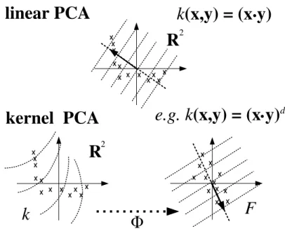
The main intuition behind this method is related to the realization of the linear PCA in some high dimensional feature space ℱ. Since ℱ is nonlinear in relation to input

space, the contour lines of constant projections onto the principal eigenvector become nonlinear in input space. Crucial to KPCA is the fact that there is no need to carry out the map into ℱ. All necessary computations are carried out by the use of a kernel

function 𝑄in the input space. Figure 3 compares the space projection on the linear PCA and KPCA.

linear PCA

kernel PCA

k

(x,y) = (x y)

R

R

k

e.g. k

(x,y) = (x y)

Φ

F

·

·

Figure 3 – The basic idea behind KPCA (SCHOLKOPF; SMOLA; MULLER, 1998).

attributes is nonlinear. The RBF kernel can be expressed by (CHANG; LIN, 2011)

𝑄(x𝑖,x𝑦) = exp (⊗Ò ‖x𝑖⊗x𝑗 ‖2), Ò >0, (2.6)

where Ò is a kernel parameter that controls the bandwidth of the inner product matrix 𝑄. An optimal value of Ò can be estimated by requiring that the corresponding inner

product matrix is maximally informative as measured by Shannon’s information entropy. The detailed steps to estimate the optimal value of Ò can be found in (REYNDERS;

WURSTEN; ROECK, 2014).

In the context of SHM, the input training matrix X is mapped by ã: X ⊃ ℱ

to a high dimensional feature space ℱ. The linear PCA is applied on the mapped data

𝒯Φ =¶ã(x1), ..., ã(x𝑛)♢. The computation of the principal components and the projection

on these components can be expressed in terms of dot products, thus the RBF kernel function can be employed. The KPCA trains the kernel data projection

U=𝐴𝑇𝑄(x) +𝑏, (2.7)

where 𝐴 is the projection matrix, 𝑏 is the bias vector and 𝑄(x) is the kernel function

centered in the training vectors. The kernel mean squared reconstruction error, which must be minimized, is defined such that

𝜀𝐾𝑀 𝑆(𝐴, 𝑏) =

1

𝑛

𝑛

∑︁

𝑖=1

where the reconstructed vector ˜ã(x) is given as a linear combination of the mapped data

𝒯Φ

˜

ã(x) =

𝑛

∑︁

𝑖=1

Ñ𝑖ã(x𝑖), Ñ =𝐴(u𝑖⊗𝑏). (2.9)

In contrast to the linear PCA, the explicit projection from the feature spaceℱ to

the input space usually does not exist (SCHOLKOPF; SMOLA, 2001).

For the test matrix Z, the residual matrix E is given by

E=ã(Z)⊗ã˜(Z), (2.10)

where ã(Z) corresponds to the high dimensional feature vectors and ˜ã(Z) their

corre-sponding reconstruction after linear PCA. The DIs are calculated using the Equation (2.4) on the residuals from E. The threshold is defined in accordance to described in

Section 2.4.2.

2.4.4 Mahalanobis squared-distance

Another well-known method for performing data normalization without any in-formation regarding the environmental and operational influences is based on the Maha-lanobis squared-distance (MSD) (WORDEN; MANSON; ALLMAN, 2003; FIGUEIREDO, 2010). The Mahalanobis distance differs from the Euclidean distance because it takes into account the correlation between the variables and it does not depend on the scale of the features. However, this model assumes that data follows a unique multivariate Gaussian distribution, i.e., the data can be modeled by only one Gaussian cluster.

Considering the training data matrixX, a mean feature vector µ and covariance

matrixΣare estimated. In the context of data normalization, the mean vector and

covari-ance matrix should encode all normal variations represented by the baseline data. Thus, for a test data z_𝑙, the MSD is used as a standard outlier analysis procedure, providing

DIs by (WORDEN, 1997)

DI(𝑙) = (z𝑙⊗µ)Σ⊗1(z𝑙⊗µ)𝑇. (2.11)

2.4.5 Gaussian mixture models

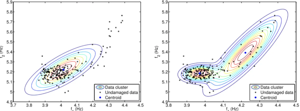
To overcome the limitations imposed by MSD, Gaussian mixture models are usu-ally employed. This algorithm carries out a model-based clustering, using multivariate finite mixture models, that aims to capture the main clusters (or components) of features that correspond to the normal and stable state conditions of a structure under operational and environmental conditions. Compared to MSD, the GMM assumes that the data can be modeled by a set of multivariate Gaussian distributions, allowing to learn nonlinear relationships (Figure 4).

f₁ (Hz)

f2

(Hz)

3.7 3.8 3.9 4 4.1 4.2 4.3 4.4 4.5 4.9 5 5.1 5.2 5.3 5.4 5.5 5.6 5.7 5.8 5.9 Data cluster Undamaged data Centroid

f₁ (Hz)

f2

(Hz)

3.8 3.9 4 4.1 4.2 4.3 4.4 4.5 4.9 5 5.1 5.2 5.3 5.4 5.5 5.6 5.7 5.8 5.9 Data cluster Undamaged data Centroid

Figure 4 – Comparison between MSD (left) and GMM (right) models (FIGUEIREDO et al., 2014a).

Therefore, a finite mixture model, 𝑝(x♣Θ), is the weighted sum of 𝐾 > 1

compo-nents 𝑝(x♣θ_𝑘) in _R𝑚,(MCLACHLAN; PEEL, 2000)

𝑝(x♣Θ) =

𝐾

∑︁

𝑘=1

Ð𝑘𝑝(x♣θ𝑘), (2.12)

whereÐ𝑘 corresponds to the weight of each component. These weights are positiveÐ𝑘 >0

with ∑︀𝐾

𝑘=1Ð𝑘 = 1. For a GMM, each component 𝑝(x♣θ𝑘) is represented as a Gaussian

distribution,

𝑝(x♣θ𝑘) =

exp{︁

⊗1₂(x⊗µ_𝑘)𝑇 Σ⊗1_𝑘 (x⊗µ_𝑘)}︁

(2Þ)𝑚/2√︁det (Σ𝑘)

, (2.13)

being each component denoted by the parameters, θ𝑘 =¶µ𝑘,Σ𝑘♢, composed of the mean

vector, µ_𝑘 and the covariance matrix, Σ𝑘. Thus, a GMM is completely specified by the

set of parameters Θ=¶Ð1, Ð2, . . . , Ð𝐾,θ1,θ2, . . . ,θ𝐾♢.

alternately applied until the log-likelihood (LogL), log𝑝(X♣Θ) = log√︂𝑛

𝑖=1𝑝(x𝑖♣Θ),

con-verges to a local optimum (DEMPSTER; LAIRD; RUBIN, 1977). The performance of the EM algorithm depends directly on the choice of the initial parameters Θ, which may

implies many replications of this method during an execution (FIGUEIREDO; JAIN, 2002). To select the best GMM by means of goodness-of-fit and parsimony, the Bayesian information criterion (BIC) is used and minimized,(BOX; JENKINS; REINSEL, 2008)

BIC =⊗2 log𝑝(X♣Θ) +

⎭ 𝐾𝑚

⎦⎤𝑚+ 1

2

⎣

+ 1⎢+𝐾⊗1

⎨

log (𝑛). (2.14)

Similar to Akaike information criterion (AIC), BIC uses the optimal LogL function value and penalizes for more complex models, i.e., models with additional parameters. The penalty term of BIC is a function of the training data size, and so it is often more severe than AIC.

For the damage detection process, and for each observation z𝑙, one needs to

esti-mate 𝐾 DIs. Basically, for each component 𝑘 discovered during training phase

DI𝑘(𝑙) = (z𝑙⊗µ𝑘)Σ⊗1𝑘 (z𝑙⊗µ𝑘) 𝑇

, (2.15)

where µ_𝑘 and Σ_𝑘 represent the parameters from all the observations of the 𝑘-th

com-ponent, when the structure is undamaged even though under varying operational and environmental conditions. Note that, each component is related to a specific source of variability (e.g., traffic loading, wind speed, temperature and boundary conditions), which allows to provide physical meanings for each component. Finally, for each observation, the DI is given by the smallest DI estimated on each component

DI(𝑙) = min (DI1,DI2,≤ ≤ ≤ ,DI𝐾). (2.16)

3 Proposed machine learning algorithms for

data normalization

In SHM, the purpose of machine learning algorithms is to enhance the damage de-tection in structures subjected to the presence of varying operational and environmental conditions under which the system response is measured. The previous chapter was ded-icated to the description of the SPR paradigm and the main statistical methods for data normalization reported in literature. Herein, two novel machine learning algorithms for statistical modeling are proposed. These approaches intend to improve the performance of traditional methods based on PCA and cluster analysis.

3.1

Deep learning algorithms

Deep learning methods aim at learning feature hierarchies of features from higher levels of the hierarchy formed by the composition of lower level features. They include learning methods for a wide range of deep architectures using graphical models with many levels of hidden variables (HINTON; SALAKHUTDINOV, 2006; BENGIO, 2009; ERHAN et al., 2010). However, the main trend of this field is based on neural networks with massive amount of hidden layers (BENGIO et al., 2007; RANZATO et al., 2007; VINCENT et al., 2008; WESTON et al., 2012).

The big challenge for development of this field concerns to the training algorithms used to build deep architectures. In virtually all instances of deep learning, the objective function is a highly non-convex function of the parameters, with the potential for many distinct local minima in the model parameter space. The main problem is that not all of these minima provide equivalent results, due to the standard training algorithms (based on random initialization) guide the searching towards areas with poor generalization per-formance (BENGIO et al., 2007).

This novel training scheme has dramatically increased the performance of such methods, driving intense research efforts to the field (ERHAN et al., 2010), mainly to the unsuper-vised branch. In this context, methods based on stacked autoencoders has demanded the main attention on the last years.

3.1.1 Autoencoders

An autoencoder is a neural network that is trained to attempt to copy its input to the output. Internally, it has a hidden layer h that describes a code used to represent

the input. The network may be viewed as consisting of two parts: an encoder function

h = 𝑓(x) and a decoder that produces a reconstruction ˆx = 𝑔(h). This architecture is

presented in Figure 5. If an autoencoder succeeds in simply learning to set 𝑔(𝑓(x)) =x

everywhere, then it is not especially useful. Instead, autoencoders are designed to be unable to learn perfectly the input patterns. This is made by adding constraints to perform only approximate copies of the input patterns into the output. Thus, the model is forced to prioritize the most important characteristics of the data, allowing to learn useful properties (GOODFELLOW; BENGIO; COURVILLE, 2016).

Figure 5 – General scheme of a simple autoencoder (GOODFELLOW; BENGIO; COURVILLE, 2016).

Traditionally, autoencoders were used for dimensionality reduction or feature learn-ing. Recently, theoretical connections between autoencoders and latent variable models have brought autoencoders to the forefront of generative modeling. A common manner to obtain useful representations is to constrainhto have smaller dimension thanx. The case

where h have a greater dimension than x has not demonstrated to result in something

The learning process is described simply as minimizing a loss function

𝐿(x, 𝑔(𝑓(x))) = 1

Ú𝑛 ∑︁

∀x_∈X

‖𝑔(𝑓(x))⊗x‖2, (3.1)

where𝐿is a loss function penalizing𝑔(𝑓(x)) for being dissimilar fromx, such as the mean

squared error, andÚis a hyperparameter which controls the asymptote slope. In this case,

an undercomplete autoencoder learns to span the principal subspace of the training data, i.e., the same subspace as PCA. Autoencoders with nonlinear encoder functions 𝑓 and

nonlinear decoder functions 𝑔 can thus learn a more powerful nonlinear generalization

than KPCA, and even better than AANN.

3.1.2 Stacked autoencoders

Multilayer autoencoders are feed-forward neural networks with an odd number of hidden layers (DEMERS; COTTRELL, 1992; HINTON; SALAKHUTDINOV, 2006) and shared weights between the encoder and decoder layers (asymmetric network structures may be employed as well). The middle hidden layer has a number of nodes equal to the number of factors to be retained, 𝑑, as in PCA. The network is trained to minimize the

mean squared error between the input and the output of the network (ideally, the input and the output are equal).

The goal of training is to perform, in the middle hidden layer (i.e., the bottleneck layer), a lower dimensional representation of the input data, in such manner that it pre-serves as much data structure as possible. The lower dimensional representation can be obtained by extracting the node values in the middle hidden layer for a given point used as input. In order to allow the autoencoder to learn a nonlinear mapping between the high-dimensional and low-dimensional data representation, sigmoid activation functions are generally used (except in the middle layer, where a linear activation function is usually employed).

The termstacked autoencoders relates to the concept of stacking simple modules of

functions or classifiers, as proposed and explored in (WOLPERT, 1992; BREIMAN, 1996; BENGIO et al., 2007), to compose a strong model. These simple models are independently trained to learn specific tasks, and then they are “stacked” on top of each other in order to learn more complex representations of the input patterns. Experimentally, stacked autoencoders yield much better dimensionality reduction than corresponding shallow or linear autoencoders (HINTON; SALAKHUTDINOV, 2006).

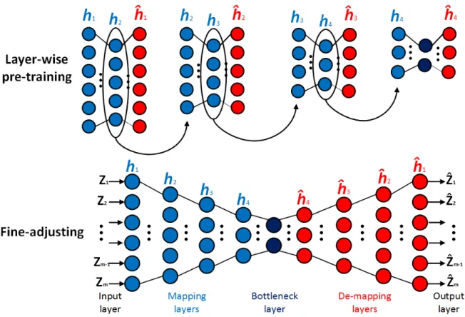
overcome these problems. An example of the two-phase training is shown schematically in Figure 6.

Figure 6 – Unsupervised layer-wise pre-training and fine adjustment of a nine-layer deep architecture.

In the context of SHM, the DSA allows to learn more reliable representations of the input vectors due to successively nonlinear transformations applied. The robust training tends to generate a more powerful model capable to generalize the normal conditions from training to the test data, performing better filtering of environmental and operational variations. Furthermore, the problems related to traditional PCA-based approaches are circumvented by this algorithm (i.e., assumptions of data normality and definition of hyper parameters are not performed). The criterion to automatically define the number of hidden nodes in each layer, as well as more details about the proposed architecture, can be found in (MAATEN; POSTMA; HERIK, 2009).

Herein, for SHM, a nine-layer DSA is trained to represent, in the bottleneck layer, low level features from training matrixX. These new features must characterize the hidden

factors that changed the underlying distribution of the structural dynamic response. For the test matrix Z, the residual matrix E is built as stated in Equation (2.5), and the

3.1.3 Deep autoencoders and traditional principal component analysis

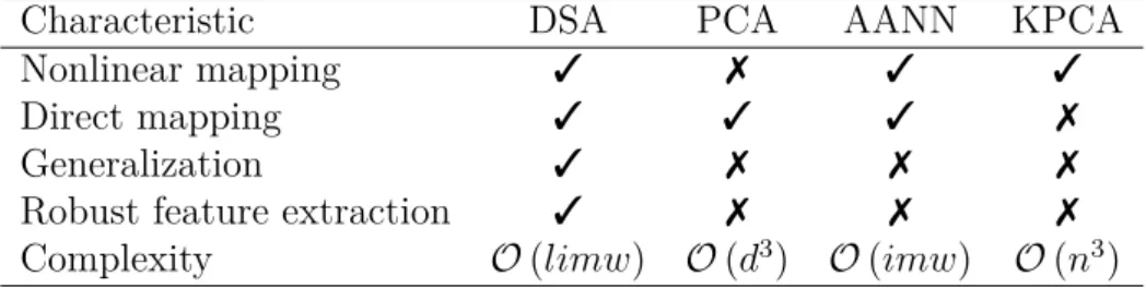
In Table 1, the approaches based on PCA are summarized by five general prop-erties: (1) ability to derive nonlinear mappings and learning nonlinear relationships in the data, (2) direct mapping between the original dimensional and the low dimensional space, (3) strengths to perform adequate learning of linear and nonlinear dependencies, (4) extraction of features that are strongly correlated to the data in original space, and (5) the computational complexity regarding the main procedures of each technique. All properties are discussed below.

Table 1 – Comparison of the different PCA-based approaches.

Characteristic DSA PCA AANN KPCA

Nonlinear mapping ✓ ✗ ✓ ✓

Direct mapping ✓ ✓ ✓ ✗

Generalization ✓ ✗ ✗ ✗

Robust feature extraction ✓ ✗ ✗ ✗

Complexity 𝒪(𝑙𝑖𝑚𝑤) 𝒪(𝑑3_{) 𝒪(𝑖𝑚𝑤) 𝒪(𝑛}3₎

The property 1 is concerned to the learning of nonlinear relationships in the data, which for real monitoring scenarios where structure dynamics is highly influenced by non-linear variations is a crucial issue. In that regard, as non-linear PCA performs only non-linear orthogonal transformations it is not able to learn, properly, nonlinear sources of varying normal conditions, resulting in inaccurate damage detection performance in many appli-cations. On the other hand, the approaches based on DSA, AANN and KPCA can handle this matter by different mechanisms, which ensure different levels of removing normal variations.

From property 2 one can infer that some techniques are not able to specify a direct mapping from the original dimension to the low dimensional space (or vice versa). It can be pointed out as a disadvantage for two main reasons: (1) it is not possible to generalize for held-out or new test data without performing a new mapping, as well as any insights about the amount of normal variability retained from the mapping/demapping operation can not be inferred. From that point of view, the approach based on KPCA is the only one that does not fall into this property, due to the learning and mapping performed in high dimensional space.

That characteristic can be assigned to the robust training phase that allows a high quality feature extraction.

One of the main qualities of deep neural networks is the robust nonlinear map-ping/demapping of data, deriving compressed representation of the input variables. In comparison, the traditional approaches to perform PCA do not allow a proper learning of the relationships between the input variables mainly due to the training algorithms and specific procedures that limit the kind of features to be extracted (e.g., linear PCA applies only orthogonal transformations, as well as the backpropagation algorithm and kernel mapping may not drive the parameter tuning towards global optimum). In that regard, property 4 indicates whether techniques provide robust mapping/demapping to compose strong features.

For property 4, Table 1 provides insight into the computational complexity of the computationally most expensive algorithmic components. The computational complexity is a issue of great importance to its practical applicability. If the memory or compu-tational resources needed are too large, their application become infeasible. Thus, the corresponding computational complexity is determined by the properties of the dataset such as the number of samples and their dimensionality, as well as the input parameters of each algorithm, such as the target dimensionality 𝑑 and the number of iterations𝑖 (for

iterative techniques). In the case of neural networks, 𝑤 indicates the size of the model by

the number of weights and 𝑙 the number of layers. The computationally most demanding

part of PCA is the eigenvalue and eigenvector decompositions, which is performed using a method in 𝒪(𝑑3_{). Due to the kernel projection, KPCA performs an eigenanalysis of an}

𝑛×𝑛 matrix by solving a semi-definite problem subjected to 𝑛 constraints, requiring a

learning algorithm in 𝒪(𝑛3_{). Both DSA and ANN employ backpropagation, which has}

a computational complexity of 𝒪(𝑖𝑚𝑤). However, as DSA has a pre-training phase, its complexity order increases to 𝒪(𝑙𝑖𝑚𝑤).

3.2

Agglomerative clustering

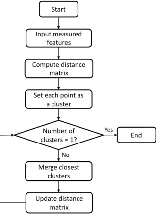
The agglomerative clustering algorithms are part of a hierarchical clustering strat-egy which treats each object as a single cluster, and iteratively merges (or agglomerates) subsets of disjoint groups, until some stop criterion is reached (e.g., number of clusters equal to one) (KAUFMAN, 1990; MAIMON; ROKACH, 2010). These bottom-up algo-rithms create suboptimal clustering solutions, which are typically visualized in the form of a dendrogram representing the level of similarity between two adjacent clusters, allowing to rebuild step-by-step the resulting merging process. Any desired number of clusters can be obtained by cutting the dendrogram properly.

Update distance matrix

End Number of

clusters = 1? Start

Input measured features

Compute distance matrix

Merge closest clusters

Yes

No Set each point as

a cluster

Figure 7 – Flow chart of agglomerative hierarchical clustering.

3.2.1 Agglomerative concentric hyperspheres

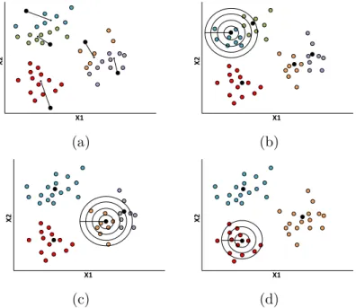
The ACH algorithm is an agglomerative cluster-based technique, working in the feature space, composed of two main steps: (1) an off-line initialization and (2) bottom-up clustering procedure. Depending on the type of initialization mechanism, the algorithm becomes completely deterministic or random. The initialization has a direct influence on the algorithm performance. Hereafter, all clusters are merged, in an iterative manner, by evaluating the boundary regions that limit each cluster through inflation of a concentric hypersphere. These two steps allow to automatically discover the number of clusters and, therefore, no input parameters are required. Note that, none information regarding data distribution is required. The entire clustering procedure is divided into three main phases:

(i) Centroid displacement. For each cluster, its centroid is dislocated to the position

with higher observation density, i.e. the mean of its observations.

(ii) Linear inflation of concentric hyperspheres. Linear inflation occurs on each centroid

by progressively increasing an initial hypersphere radius,

𝑅0 = log10

⎞

‖c𝑖⊗x𝑚𝑎𝑥‖2 + 1

⎡

, (3.2)

where c𝑖 is the centroid of the 𝑖-th cluster, used as a pivot, and x𝑚𝑎𝑥 is its farthest

observation, such that ‖c_𝑖⊗x_𝑚𝑎𝑥‖2 is the radius of the cluster centered in c_𝑖. The

radius grows up in the form of an arithmetic progression (AP) with common differ-ence equal to 𝑅0. The creation of new hyperspheres is set by a criterion based on

the positive variation of the observation density between two consecutive inflations, defined as the inverse of variance; otherwise the process is stopped.

(iii) Cluster merging. If there is more than one centroid inside the inflated hypersphere,

all centroids are merged to create an unique representative centroid positioned at the mean of the centroids’ position. On the other hand, if only the pivot centroid is within the inflated hypersphere, this centroid is assumed to be on the geometric center of a cluster, thus the merging is not performed.

X2

X1

(a)

X2

X1

(b)

X2

X1

(c)

X2

X1

(d)

Figure 8 – ACH algorithm using linear inflation running in a three-component scenario.

infer if the new one is not badly positioned in another cluster or closer to a boundary region.

The Algorithm 1 summarizes the proposed method. Initially, it identifies the clus-ter to which each observation belongs and moves the centroids to the mean of their observations. Then, a hypersphere is built on the pivot centroid and it is inflated until the observation density decreases. Finally, the merges of all centroids within the hypersphere is performed, by replacing these centroids by their mean. The process is repeated until convergence, i.e. there is no centroid merging after the evaluation of all centroids or the final solution is composed by only one centroid.

Note that, the main goal of the clustering step is to maximize the observation density related to each cluster. In other words, to locate the positions with maximum observation concentration, also known as mass center, in such manner that when a hyper-sphere starts to inflate its radius, it reaches the decision boundaries of the cluster. This process is also described by maximizing the cost function

max ∑︁𝐾

𝑘=1

⎠ ∑︁

xi∈ck

‖x𝑖⊗c𝑘‖2 N𝑘

⎜⊗1

,

s.t. 𝑛=

𝐾

∑︁

𝑘=1

N𝑘,

1⊘N𝑘 ⊘𝑛,

(3.3)

where c_𝑘 is the𝑘-th centroid,x_𝑖 the 𝑖-th observation assigned to the𝑘-th cluster andN_𝑘

is the number of observations in the cluster 𝑘. The clustering procedure naturally carries