221 (2010) 423–427
Contents lists available atScienceDirect
Ecological Modelling
j o u r n a l h o m e p a g e :w w w . e l s e v i e r . c o m / l o c a t e / e c o l m o d e l
Modelling environmental stochasticity in adult survival for a long-lived species
Ari Samaranayaka
∗, David Fletcher
Department of Mathematics and Statistics, University of Otago, Dunedin, New Zealand
a r t i c l e
i n f o
Article history: Received 21 July 2009
Received in revised form 3 October 2009 Accepted 7 October 2009
Available online 10 November 2009
Keywords: Beta distribution
Environmental stochasticity Logit-normal
Matrix population model Probit-normal
a b s t r a c t
Stochastic matrix population models are often used to help guide the management of animal populations. For a long-lived species, environmental stochasticity in adult survival will play an important role in deter-mining outcomes from the model. One of the most common methods for modelling such stochasticity is to randomly select the value of adult survival for each year from a distribution with a specified mean and standard deviation. We consider four distributions that can provide realistic models for stochasticity in adult survival. For values of the mean and standard deviation that cover the range we would expect for long-lived species, all four distributions have similar shapes, with small differences in their skewness and kurtosis. This suggests that many of the outcomes from a population model will be insensitive to the choice of distribution, assuming that distribution provides a realistic model for environmental stochas-ticity in adult survival. For a generic age-structured model, the estimate of the long-run stochastic growth rate is almost identical for the four distributions, across this range of values for the mean and standard deviation. Model outcomes based on short-term projections, such as the probability of a decline over a 20-year period, are more sensitive to the choice of distribution.
© 2009 Elsevier B.V. All rights reserved.
1. Introduction
Matrix models are often used to help guide the management of animal populations (Boyce, 1992; Beissinger and Westphal, 1998; Caswell, 2001). When there is environmental stochasticity (here-after referred to simply as stochasticity) in one or more of the demographic parameters, use of a stochastic model will be prefer-able to use of a deterministic one (Shaffer, 1987; Soulé, 1987; Burgman et al., 1993; Caswell, 2001; Engen et al., 2001).
For the population model we consider later (Section 3), preliminary analysis suggested that the results obtained from incorporating stochasticity in one of the parameters (such as adult survival) would not depend greatly on the values of the other parameters. This implied that we could therefore focus on modelling stochasticity in adult survival alone, with all other parameters fixed, as this is the parameter for which a specified amount of stochasticity has the largest impact on the stochastic growth rate for a long-lived species (Tuljapurkar, 1982). Stochas-ticity in adult survival can be modelled in a number of ways, one of the most common methods being to randomly select the value of adult survival for each year from a statistical distribution (Fieberg and Ellner, 2001; Kaye and Pyke, 2003; Dias et al., 2008). The distribution will often be specified in terms of its mean () and
∗ Corresponding author. Current address: Injury Prevention Research Unit, Uni-versity of Otago, Dunedin, New Zealand. Tel.: +64 34797168; fax: +64 34798337.
E-mail address:[email protected](A. Samaranayaka).
standard deviation (). For long-lived species, these values might come from an analysis of mark-recapture data (Gould and Nichols, 1998; Burnham and White, 2002), or from fitting the population model directly to census and mark-recapture data (Buckland et al., 2004, 2007; Thomas et al., 2005). Whatever methods are used, esti-mation ofcan be prone to problems if there are only a few annual estimates and/or these are poorly estimated. In such casesmay need to be arbitrarily specified, perhaps using information from other long-lived species (Breen et al., 2003).
However we determine appropriate values forand, there is some choice as to the form of the distribution to use to model the stochasticity. The purpose of this paper is to consider the extent to which the form of this distribution has an impact on the results from the population model. If two distributions have the same shape they will obviously provide the same results from the popu-lation model. If they have the same mean and standard deviation, any difference between the model results will be due to differ-ences in their higher-order moments, particularly skewness and kurtosis (Slade and Levenson, 1984; Tuljapurkar, 1990; Wiener and Tuljapurkar, 1994). It is therefore of interest to compare the skewness and kurtosis of distributions that might provide realistic models of environmental stochasticity in adult survival.
Previous work in this area has focussed on distributions that were either similar or markedly different in shape (and there-fore in higher-order moments), and the results reported seem to reflect this. ThusFieberg and Ellner (2001)found that the choice of distribution had little effect on the results they obtained from a pop-ulation model that incorporated stochasticity in all the parameters,
424 A. Samaranayaka, D. Fletcher / Ecological Modelling221 (2010) 423–427
and noted that this was not surprising as the distributions they con-sidered were either symmetric or close to symmetric. Conversely,
Slade and Levenson (1984)found that using two distributions with quite different shapes (symmetric or negatively skewed) to model stochasticity in juvenile survival had an effect on the results from their population model. Likewise,Nakaoka (1997)found that use of a truncated-normal or a lognormal distribution to model stochas-ticity in recruitment led to quite different results.Kaye and Pyke (2003)also found that distributions with quite different shapes could lead to different estimates of stochastic population growth rate and population viability.
We argue that any comparison between distributions should involve only those that have the ability to match the shape of the distribution of annual estimates of the relevant parameter, or a shape that is considered appropriate for the population. In the case of adult survival,Dias et al. (2008)suggest that a unimodal distribution will usually be appropriate, and that a J-shaped or U-shaped distribution may sometimes be considered. Although they have been used in the past, it is clear that a truncated distribution cannot provide a realistic model for stochasticity in a demographic parameter (Nakaoka, 1997; Wade, 1998; Higgins et al., 2000). In addition naïve use of truncation can lead to the distribution differ-ing markedly from what was intended (Caswell, 2001; Fieberg and Ellner, 2001; Todd and Ng, 2001; Kaye and Pyke, 2003; Dias et al., 2008).
In comparing the effects of two distributions, it is also impor-tant to consider the type of outcome from the population model. A natural outcome to consider is the stochastic growth rate, defined as
logs= lim
t→∞ 1
t logNt
whereNtis the population size in yeart(Caswell, 2001). It is
com-mon to estimate logsby calculating the mean annual growth rate
over a suitably long period (Tyears), i.e. by
1 T
T−1
t=0
rt
wherert=log
Nt+1/Nt. Estimation of logstherefore involvesuse of a sample of sizeTfrom the distribution for adult survival, whereTis very large. If two distributions for adult survival have similar shapes, the two samples of values for adult survival will be similar, thereby leading to the two estimates of logsbeing close.
Another way of seeing this is to consider a standard approxima-tion to logs(Caswell, 2001, p. 398). For the population model we
consider in Section3, this approximation can be written as
logs≈log−1 2
5−4 2where is the population growth rate for the corresponding deterministic model (i.e. with= 0). This result suggests that two distributions with the same values forandwill lead to similar estimates of logs, any differences being related to the terms
miss-ing from this approximation, which involve higher-order moments such as skewness and kurtosis (Tuljapurkar, 1990; Wiener and Tuljapurkar, 1994).
An alternative type of outcome to consider is one based on short-term projections, such as the probability of a population decline over a 20-year period. This can be estimated by projecting the pop-ulation for 20 years a large number of times and calculating the proportion of these replicate projections for which the population size declined. In this context, the “sample size” taken from the distribution for adult survival is relatively small for each projec-tion, but the overall “sample size” will usually be large, due to the number of replicate projections used in the estimation.
Regardless of the type of model outcome considered, little is currently known about how close such outcomes might be for two realisticdistributions for modelling stochasticity in adult survival for a long-lived species. In Section2we describe four such distri-butions, and compare their skewness and kurtosis over a range of values forandthat are relevant to long-lived species. In Sec-tion3we compare the effect they have on the results from a generic population model for such a species. Section4contain the results and discussion.
2. Candidate distributions
As we have argued above, a realistic distribution for adult sur-vival should allow one to specify a unimodal, J-shaped or U-shaped distribution (the latter corresponding to the case where we wish to use a distribution to model the occurrence of “catastrophic” years). In addition, it is clear that use of a truncated distribution is not appropriate.Dias et al. (2008)make a strong case for the beta dis-tribution as the default choice for modelling stochasticity in any demographic parameter. This has the following probability density function (pdf) on the (0,1) interval:
f(s)=s
˛−1(1−s)ˇ−1
B(˛, ˇ)
0< s <1;˛, ˇ >0
where˛andˇare the parameters andB(˛,ˇ) is the beta function (Johnson et al., 1994). There are many examples of this distribution being used to model stochasticity (e.g. Kendall, 1998; Grevstad, 1999). For the purposes of this paper, we consider the beta dis-tribution as a benchmark against which the others are compared. A natural alternative to the beta distribution is the logit-normal distribution, as its use implies that adult survival has a normal distribution on the logit-scale, an assumption that is often made when analysing mark-recapture data, especially when modelling survival in terms of covariates (Newman, 2003). Using this dis-tribution means that the survival rateScan be generated using S= (1 + e−X)−1, whereX∼N
X, X2
, and the pdf forSis given byf(s)= 1
(2)1/2s(1−s)X exp
−(logit(s)−X)2 2X2
(0< s <1; >0)
A distribution that is closely related to the logit-normal is the probit-normal.Todd and Ng (2001)promoted use of this distribu-tion in the case where one wants to incorporate cross-correladistribu-tion amongst different demographic parameters. Recently, however,
Dias et al. (2008)have shown that the beta distribution can also be used when there is a need to model such correlation, poten-tially obviating the need for the probit-normal. We include it here for the sake of completeness. The probit-normal is based on the assumption that survival will have a normal distribution on the probit-scale, i.e. the survival rateScan be generated usingS=˚(X), whereX∼N
X, X2and˚(.) is the cumulative distribution func-tion for the standard normal distribufunc-tion. The pdf forSis given byf(s)= 1
X
˚−1(s)˚−1(s)− X X
(0< s <1;X>0)
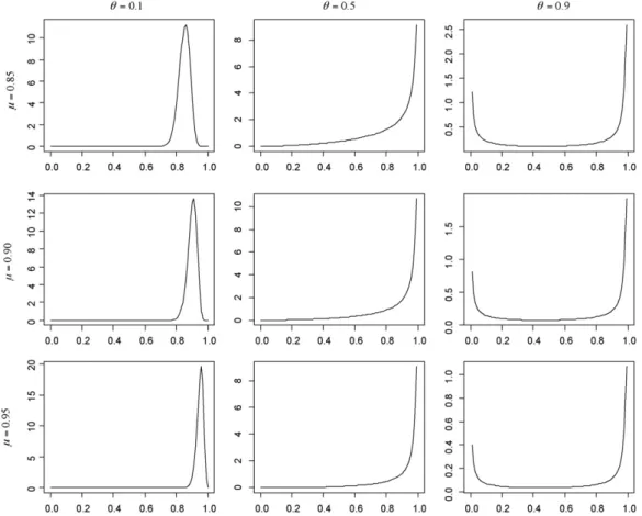
Fig. 1.The beta probability density function, for nine combinations of the mean () and=/ (1−), whereis the standard deviation.
whereX∼N
0, X2and 0 < < 1, and the pdf forSis given byf(s)= 1
(2)1/2sln
s−1X
exp
−1 22 X
ln
ln(s) ln( ) 2(0< s <1;X>0)
Suppose we estimateandin a preliminary analysis, i.e. we do not fit a population model directly to data (Section1). Use of the beta distribution then has the advantage that we can specify the parameters directly in terms ofand:
˛=
(1−)2 −1
, ˇ= (1−)˛
For the logit-normal, probit-normal and lognormal-power, there are no exact expressions forand (nor for any higher-order moments). Note that it might sometimes be convenient to specifyandon the logit-scale, in which case calculation of the parameters for the logit-normal would be exact, while those for the beta would not. We used the following numerical procedure to calculate the parameter values, given target values (TandT) for
and:
(1) Specify initial values for the parameters of the distribution (see below)
(2) Randomly select 106observations from the specified
distribu-tion, and calculate their mean (m) and standard deviation (S) (3) Calculate the sum of the absolute relative errors inand, i.e.
e=
m−T
T
+s−T
T
(4) Repeat Steps 2 and 3 until e is suitably small, using an optimi-sation algorithm to vary the values ofand.
All calculations were carried out inR Version 2.8.0 (2008), and we implemented the procedure using theoptim command. This command makes use of the Nelder–Mead simplex method for optimisation (Nelder and Mead, 1965). In order to speed up con-vergence, we used the same random seed each time Step 2 was invoked. We used Taylor series approximations to specify the initial values for the parameters (Samaranayaka, 2005). For each distribu-tion and for each pair of values (T,T), we replicated the procedure
ten times and used the mean estimate for each parameter.
3. Comparison of model outcomes
We considered an age-classified population model that is appli-cable to many long-lived species. It is based on a pre-breeding census, and age at first reproduction isafor all individuals, i.e. there area−1 juvenile stages, and one adult stage. Adults that survive remain in the final stage, and both fertility and adult survival are assumed to be independent of age. Preliminary analysis suggested that our results would be robust to the choice ofa, which we arbi-trarily set to 5 years. All parameters other than adult survival were assumed to be constant. The projection matrix associated with this model is given by
⎡
⎢
⎢
⎣
0 0 0 0 fs0
s1 0 0 0 0
0 s2 0 0 0
0 0 s3 0 0
0 0 0 s4 sA(t)
426 A. Samaranayaka, D. Fletcher / Ecological Modelling221 (2010) 423–427
Table 1
Estimates of the probability of a population decline over 20, 50 or 100 years for a population model, using four distributions to model stochasticity in adult survival. Each estimate has a standard error of less than 0.002.
Beta Logit-normal Probit-normal Lognormal-power
20 years
0.85 0.1 1.000 1.000 1.000 1.000
0.85 0.5 0.972 0.972 0.973 0.974
0.85 0.9 0.915 0.914 0.916 0.917
0.90 0.1 0.987 0.988 0.987 0.988
0.90 0.5 0.711 0.703 0.706 0.690
0.90 0.9 0.766 0.766 0.765 0.773
0.95 0.1 0.000 0.000 0.000 0.000
0.95 0.5 0.144 0.158 0.151 0.182
0.95 0.9 0.453 0.454 0.457 0.478
50 years
0.85 0.1 1.000 1.000 1.000 1.000
0.85 0.5 0.999 0.999 0.999 0.999
0.85 0.9 0.984 0.984 0.984 0.984
0.90 0.1 1.000 1.000 1.000 1.000
0.90 0.5 0.838 0.832 0.835 0.827
0.90 0.9 0.860 0.861 0.862 0.863
0.95 0.1 0.000 0.000 0.000 0.000
0.95 0.5 0.059 0.071 0.068 0.104
0.95 0.9 0.374 0.378 0.377 0.380
100 years
0.85 0.1 1.000 1.000 1.000 1.000
0.85 0.5 1.000 1.000 1.000 1.000
0.85 0.9 0.999 0.999 0.999 0.999
0.90 0.1 1.000 1.000 1.000 1.000
0.90 0.5 0.924 0.923 0.923 0.919
0.90 0.9 0.943 0.945 0.942 0.943
0.95 0.1 0.000 0.000 0.000 0.000
0.95 0.5 0.016 0.024 0.020 0.045
0.95 0.9 0.351 0.356 0.357 0.364
wherefis the reproductive rate (newborns per adult),Siis the
sur-vival rate from ageitoi+ 1 (i= 0, 1, 2, 3, 4), andSA(t) is the adult
survival rate from yearttot+ 1 (t= 0, 1, 2,. . .).
The preliminary analysis referred to earlier (Section 1) sug-gested that our results would be robust to the choices of f and Si (i= 0, 1, 2, 3, 4), so we arbitrarily set f= 0.3,S0= 0.7 and
Si= 0.8 (i= 1, 2, 3, 4). We considered three values for the mean
of the adult survival rate (), covering the range we would expect for long-lived species: 0.85, 0.90 and 0.95. In choosing suitable values for the standard deviation of the survival rate (), we used the fact that it cannot exceed (1−) (Dias
et al., 2008). Thus we set = (1−) with = 0.1, 0.5 or 0.9, corresponding to low, medium and high levels of stochas-ticity, respectively. These three values of lead to the beta distribution being unimodal, “J-shaped” and “U-shaped”, respec-tively.
We considered two types of outcome from the population model. The first was the long-run stochastic growth rate, logs,
defined in Section1. The standard error of the estimate of logs
was calculated as V/T, whereVis the sample variance of the rt (t= 0, 1,. . .,T−1) (Caswell, 2001). We usedT= 106, as this led to the standard error being less than 0.0001 for each of the sce-narios we considered. We arbitrarily setN0= 1, and the initial age
distribution was set equal to the stable age distribution for the cor-responding deterministic model. The second type of outcome we considered was the probability of a decline in population size in the short-term, i.e. after 20, 50 and 100 years. We estimated these probabilities by repeatedly projecting the model over the relevant time period, using the same initial conditions as for estimation of the long-run growth rate. We chose to use 105replicates for this
purpose, in order to ensure that the binomial standard error of the estimated probability would be less than 0.002.
4. Results and conclusions
For the range of values considered forand, the four distri-butions have similar shapes. For all four distridistri-butions,= 0.1, 0.5 and 0.9 correspond to unimodal, “J-shaped” and “U-shaped” distri-butions, respectively.Fig. 1shows the beta distribution for each combination ofand: the other three distributions are close enough in shape to the beta that we have not plotted them, for ease of presentation. The degree of similarity across the four distribu-tions can be gauged by considering the relative absolute difference between the first four moments of the beta distribution and those for the other three distributions, using the samples of size 106that
were generated in order to estimate logs: across the range of
val-ues considered forand, these relative differences are all less than 0.0005.
For each of the nine combinations ofand, the estimates of the long-run stochastic growth rate (logs) were identical for the
four distributions (to three decimal places). As predicted, this esti-mate is thus extremely robust to the choice of distribution. The differences between the distributions might be explained by dif-ferences in their higher-order moments, but could also be due to numerical differences in their means and standard deviations, as a result of the numerical procedure used to estimate the param-eters for the logit-normal, probit-normal and lognormal-power distributions. A general linear model for the estimate of logsin
terms of the realised mean and standard deviation of the corre-sponding distribution (i.e. from the sample of size 106) fitted better
than one involving all of the first four moments (the difference in AIC being 2.25). This implies that differences in the mean and standard deviation, caused by errors in estimating the parameters for the logit-normal, probit-normal and lognormal-power, were more influential than differences in skewness and kurtosis (c.f.
Estimates of the probability of population decline over 20, 50 and 100 years are given inTable 1. These are also fairly robust to the choice of distribution, with the estimates for the logit-normal, probit-normal and lognormal-power all being within five percent-age points of the corresponding estimate for the beta distribution. The largest differences are for the lognormal-power, especially when the distribution is J-shaped or U-shaped (= 0.5 or 0.9). If the distribution is unimodal (= 0.1) the differences are negligible. Overall, our results suggest the outcomes from a stochastic matrix population model for a long-lived species will be robust to the choice of distribution used to represent stochasticity in adult survival, as long as that distribution provides a realistic model for such stochasticity. As adult survival is the parameter for which a specified amount of stochasticity has the largest impact on the stochastic growth rate, we would expect similar results for the survival rates of other age classes.
References
Beissinger, S.R., Westphal, M.I., 1998. On the use of demographic models of population viability in endangered species management. Journal of Wildlife Management 62, 821–841.
Boyce, M.S., 1992. Population viability analysis. Annual Review of Ecology and Sys-tematics 23, 481–506.
Breen, P.A., Hilborn, R., Maunder, M.N., Kim, S.W., 2003. Effects of alternative control rules on the conflict between a fishery and a threatened sea lion (phocarctos hookeri). Canadian Journal of Fisheries and Aquatic Sciences 60, 527–541. Buckland, S.T., Newman, K.B., Thomas, L., Koesters, N.B., 2004. State-space models for
the dynamics of wild animal populations. Ecological Modelling 171, 157–175. Buckland, S.T., Newman, K.B., Fernández, C., Thomas, L., Harwood, J., 2007.
Embed-ding population dynamics models in inference. Statistical Science 22, 44–58. Burgman, M.A., Ferson, S., Akcakaya, H.R., 1993. Risk Assessment in Conservation
Biology. Chapman and Hall, London.
Burnham, K.P., White, G.C., 2002. Evaluation of some random effects methodology applicable to bird ringing data. Journal of Applied Statistics 29, 245–264. Caswell, H., 2001. Matrix Population Models, Construction, Analysis, and
Interpre-tation, second ed. Sinauer Associates Inc.
R Development Core Team, 2008. R: A Language and Environment for Statistical Computing. R Foundation for Statistical Computing, Vienna, Austria. ISBN 3-900051-07-0, URLhttp://www.R-project.org.
Dias, C.T.D.S., Samaranayaka, A., Manly, B., 2008. On the use of correlated beta ran-dom variables with animal population modelling. Ecological Modelling 215, 293–300.
Engen, S., Saether, B.E., Moller, A.P., 2001. Stochastic population dynamics and time to extinction of a declining population of barn swallows. Journal of Animal Ecology 70, 789–797.
Fieberg, J., Ellner, S.P., 2001. Stochastic matrix models for conservation and management: a comparative review of methods. Ecology Letters 4, 244–266.
Gould, W.R., Nichols, J.D., 1998. Estimation of temporal variability of survival in animal populations. Ecology 79, 2531–2538.
Grevstad, F.S., 1999. Factors influencing the chance of population establishment: implications for release strategies in biocontrol. Ecological Applications 9 (4), 1439–1447.
Higgins, S.I., Picket, S.T.A., Bond, W.J., 2000. Predicting extinction risk for plants: environmental stochasticity can save declining populations. TREE 15, 517– 521.
Johnson, N.L., Kotz, S., Balakrishnan, N., 1994. Continuous Univariate Distributions-V2. John Wiley & Sons Inc., New York.
Kaye, T.N., Pyke, D.A., 2003. The effect of stochastic technique on estimates of population viability from transition matrix models. Ecology 84, 1464– 1476.
Kendall, B.E., 1998. Estimating the magnitude of environmental stochasticity in sur-vivorship data. Ecological Applications 8, 184–193.
Nakaoka, M., 1997. Demography of marine bivalve Yoldia notabilis in fluctuat-ing environments: an analysis usfluctuat-ing a stochastic matrix model. Oikos 79, 59– 68.
Nelder, J.A., Mead, R., 1965. A simplex algorithm for function minimization. Com-puter Journal 7, 308–313.
Newman, K.B., 2003. Modelling paired release-recovery data in the presence of sur-vival and capture heterogeneity with application to marked juvenile salmon. Statistical Modelling 3, 157–177.
Samaranayaka, A., 2005. Environmental Stochasticity and Density Dependence in Animal Population Models. Ph.D. Thesis. University of Otago, Dunedin. Shaffer, M.L., 1987. Minimum viable populations: coping with uncertainty. In: Soulé,
M.E. (Ed.), Viable Populations for Conservation. Cambridge University Press, New York.
Slade, N.A., Levenson, H., 1984. The effect of skewed distributions of vital statis-tics on growth of age-structured populations. Theor. Popul. Biol. 26, 361– 366.
Soulé, M.E., 1987. Viable Populations for Conservation. University of Cambridge, Cambridge.
Thomas, L., Buckland, S.T., Newman, K.B., Harwood, J., 2005. A unified framework for modelling wildlife population dynamics. Australian and New Zealand Journal of Statistics 47, 19–34.
Todd, C.R., Ng, M.P., 2001. Generating unbiased correlated random survival rates for stochastic population models. Ecological Modelling 144, 1–11.
Tuljapurkar, S.D., 1982. Population dynamics in variable environments. II. Correlated environments, sensitivity analysis and dynamics. Theoretical Population Biology 21, 114–140.
Tuljapurkar, S.D., 1990. Population Dynamics in Variable Environments. Lecture Notes in Biomathematics, Number 85. Springer, New York.
Wade, P.R., 1998. Calculating limits to the allowable human-caused mortality of Cetaceans and Pinnipeds. Marine Mammal Science 14, 1–37.