Simulation-based smoothing and filtering in factor stochastic volatility models : two econometric applications

(1)

Time-Varying Covariance Structures in Currency Markets

Hedibert Freitas Lopes

Universidade Federal do Rio de Janeiro

Ornar Aguilar

Merryl Lynch Quantitative Research

Mike West

Duke University

July 2000

Abstract

In this article we use factor models to describe a certain class of covariance structure for financiaI time series models. More specifical1y, we concentrate on situations where the factor variances are modeled by a multivariate stochastic volatility structure. We build on previous work by allowing the factor loadings, in the factor mo deI structure, to have a time-varying structure and to capture changes in asset weights over time motivated by applications with multi pIe time series of daily exchange rates. We explore and discuss potential extensions to the models exposed here in the prediction area. This discussion leads to open issues on real time implementation and natural model comparisons.

Keywards: Bayesian inference, latent factor models, time-varying loadings, non-Gaussian dynamic models, stachastic volatility components.

1 Introduction

Factor models have received great academic attention since the early days at the beginning of the century with the work of Spearman (Bartholomew, 1995). However, until recent1y, with the advent of powerful and fast computer machinery, factar models have received less than full attention of practitioners. These models are now emerging in problems in the fields as diverse as geology, credit analysis, and financiaI markets among others. This paper applies factor mo deIs to characterize covariance structures in certain classes of multivariate stochastic volatility models, or more specifically, factor stochastic volatility mo deIs (FSV), with a particular view to applications in economics and finance.

(2)

and Kim et alo (1998). Although generalizations to multivariate situations are theoretically

and conceptually simple, academics and practicioners experienced computational problems with the statistical inference. Many attempts have been made to overcome dimensionality problems and factor mo deIs opened the possibility to solve the problems for the same reasons stressed above.

Diebold and Nerlove (1989) introduce the latent factor ARCH models, which is further explored and compared with other variance models in Sentana (1998) and Giakoumatos et alo (1999). The former studied the differences between Diebold and Nerlove's latent factor

ARCH mo deIs and Engle (1987)'s factor ARCH models, while the latter compared a latent one-factor ARCH model with Shephard's unobserved ARCH model.

The works of Harvey

et

alo (1994) followed by Jacquier

et

alo (1995) and Kim

et

alo

(1998), and more recently by Aguilar and West (2000) and Pitt and Shephard (1999), form the basis for the model developments we consider. They basically model the leveIs of a set of time-series by a factor mo deI where both the common factor variances and the specific (or idiosyncratic) variances follow multivariate and univariate first order stochastic volatility structures respectively.

We build on these works in some theoretical and practical directions by allowing the factor loadings to evolve in time. The rationale behind these extensions is that by allowing the factor loadings to change over time we maintain the factor scores interpretability virtually the same across time and give more felixibility to the model. In other words, our model incorporates the idea that the weight that some factors have on a particular time series might change with time, mimicking real financial/ economic scenarios. A simple example is when a country (or countries) enter/leave a particular market, and when such a market is

been represented by a group of stable latent factors. Moreover, in a more general framework and with the current global market integration, financiaI and economic indicators tend to be driven by latent factors which importance is constantly changing. This is dear in currency markets and in some equity markets as well, specially in the euro-zone.

The rest of the article is organized as follows. Section 2 sets up the mo deI which has two major components. In the first component, a factor model is used to represent the leveI of time series dependence structure where we allow the loadings matrix to change overtime by specifying a stochastic evolution processo In the second component, we follow previous work on multivariate stochastic volatily mo deIs by specifying multi pIe time series mo deIs for the log volatilityes of the common factors. In this section, we also setup the environmet for Bayesian inference and we lay down the prior distributions for the model's parameters.

(3)

2 Model and Prior

As is traditional in the factor analysis context, we assume that Yt is a m-dimensional vector of time series, whose leveIs follow a k-factor model,

(1)

where, again, "Yt is the m-dimensional mean leveI vector, {3t is the m x k factor loading matrix,

f

t is the k x 1 vector of common factors and :Et is the m x m diagonal matrix with the specific or idiosyncratic variances. The main departures from stantard factor analysis lie in the time structure of the parameters in "Y, {3,:E and the variances of

f.

We assume that the mean leveI, "Yt follows a simple multivariate random walk process of the following form,

(2)

to capture constant local (myopic) leveIs in the series. We will further assume that the evolution matrices

Wl

are completely specified by a single and known discount factor 8"( E

(0,1), see West and Harrison (1997) for further details. We also assume the common factors are independent and normally distributed over time, conditional on Ht,

(3)

with H t

=

diag(hlt , ... , hkt ). Following Aguilar and West (2000) model, the log-volatilities

Àit = log(hit), can be described by a multivariate first-order autoregressive (VAR) model

with correlated innovations,

(4)

for Àt

=

(À_{lt , ... ,}À_{kt )',}a

=

(aI, ... , ak)', and cp

=

diag(qh, ... , <Pk).

We also assume that the persistance parameters O

<

<Pi

<

1 for i

=

1, ... ,k, to guarantee non-explosive behaviour in the final time series variances and covariances and representing real life volatility clusters. These assumptions also imply that changes in variances in a period of time are most certainly followed by consecutive changes in the same direction in the near future, an assumption that is fairly reasonable and observed quite oftenly in practice. Moreover, by allowing correlated innovations in the time series model we are capturing the potential high leveIs of correlations observed in periods of high financial stress and volatility peaks, Aguilar and West (2000). Under such assumptions, it is easy to see that ÀI rv N(IL, W), where W satisfies W

=

cpWcjJ+

u.

On the other hand, univariate stochastic volatility structures are asumed for the non-zero elements of :Et = diag(art, . .. ,

a~t) in the same fashion as in Jacquier et alo (1995), Pitt and Shephard (1999) and Aguilar and West (2000). More specifically, the idiosyncratic log-volatilities, TJit = log(a;t) follow

standard first-order autoregressive models,

('Tltl'Tlt-l, õ, p, S) rv N(õ

+

P('Tlt-1 - õ); S) (5)

(4)

The major component of this work and a huge departure from traditional factor models and for current stochastic volatility models is to allow the loadings to change overtime and hence capturing the changes in importance of the latent factors in a more realistic fashion. In particular, due to identification contraints, the loading matrices, (3t, are block lower triangular, i.e. /3ij,t

=

O for alI j

>

i and ones in the main diagonal. To setup the evolution for the ~nconstrained elements of (3t we stacked them up in a d = mk-k(k-1)j2 dimensional vector f3t = (/321,t, /331,t, ... ,/3n,k,t), that follows a first-order autoregression evolution for the

unconstrained loadings,

(6)

with ,

=

((1, ... ,(d), ~

=

diag(61 , ... , 6d).

We will further assume that the evolution matrices

wf

are completely specified by a single and known discount factor 6{3 E (0,1). Basically, a discount factor will measure the decay or loss of information incurred in the updating mechanism. Discount factors dose to one wiIl tend to model relatively small changes in the state vector, in our case, the loadings. On the other hand, big changes in the evolution of the state vector are better described by smaIler discount factors. See West and Harrison (1997) for further details.

Note that by allowing time-varying structures in the loadings matrix we are extending previous model structures that can be summarized as follows,

1. 6,

=

6{3

=

1: Aguilar and West's dynamic factor model;

2. Uij

=

O for i

=I

j, 6,

=

6{3

=

1: Pitt and Shephard's factor stochastic volatility model;

3. U = O, S = O recovers the traditional static factor model (Geweke and Zhou, 1996).

In order to complete the requisites for the Bayesian analysis, prior distributions must be defined and we will restrict our analyses to conditionaIly conjugate prior distributions to facilitate the already complicated posterior analysis. To begin with, the prior distribution for the time series mean leveI at time

t

=

1 is ;1 f"V N(;o, Eo), for ;0 and Eo known hyperparameters. Analogously, the prior distribution for the unconstrained loadings at time t = 1 is (jo f"V N(mo, Co), with mo and Co known hyperparameters. The prior distributions for components of' and the nonzero components ~ are ( j f"V N((oj, COj ) and 6_j f"V N(6oj , VOj ) , respectively, for j = 1, ... , d.

For the parameters that define both the factors's log-volatility equations,

0:,4>,

U, and the idiosyncratic factors's log-volatility, li , p, s, we follow Aguilar and West (2000) sugges-tions. They assume independent normal priors for the univariate terms of o: and li and independent truncated normal priors for the terms in

4J

and p. Inverted Wishart and in-verted gamma distributions are assigned to U and to the diagonal elements of S, respectively. More specifically, U f"V IW(ro, roRo) and Si f"V IG(vod2, vOi S5d2), para i = 1, ... , m with

ro,

Ro,

VOi and S5i given hyperparameters.

Posterior analysis is attained by applying an hybrid Markov chain Monte Carlo sampler that was tailored for the model presented. The sampler combines methodology developed by various authors that dealt with similar models. See Aguilar and West (2000), Pitt and Shephard (1999) and Lopes (2000) for technical details and further references.

(5)

3 Daily exchange rate returns

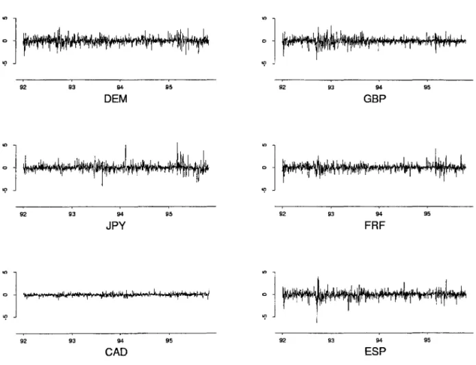
We analyse the sarne dataset used in Aguilar and West (2000), narnely the returns on week-day closing spot prices for six currencies relative to the US dollar. The dataset eontains 2872 observations that range from 12/31/1987 to 01/01/1999. We will foeus most of our analysis to the stretch of 1000 observations that goes from 1/1/1992 to 10/31/1995. AIso, the observations will be transformed in order to use one-day-ahead returns. Figure 1 shows the transformed time series in the order used by Aguilar and West (2000): German Mark (DEM), British Pound (GBP), Japanese Yen (JPY), Freneh Frane (FRF), Canadian Doliar (CAD) and Spanish Peseta (ESP).

3.1 Exploratory analysis

The naive fit of a 3-factor model to the data yields the following esimates for the loading matrix and for the idiosyneratic varianees:

1.00 0.00 0.00 2.92

0.74 1.00 0.00 9.96

(3= 0.72 -0.39 1.00 and 106~ = diag 2.66

0.96 0.05 0.00 2.34

-0.05 0.24 -0.08 8.54

0.87 0.39 -0.08 12.69

These are erude estimates whieh do not take into eonsideration any time-varying strueture for the time series eovarianee. Nevertheless, they point out some interesting direetions. Firstly, it seems that GBP, DEM, FRF and ESP are fairly eorrelated. Seeondly, CAN does not seem to be eorrelated to any of the other returns, while JPY time seems to be eorrelated with DEM, FRF and ESP. Thirdly, the first factor weights (first eolumn of the factor loading matrix) has basically the same strueture when one, two or three factor models are fitted to the data, in which DEM, GBP, FRF and ESP have dominating influenee, with JPY having minor influenee and CAD plaeing no influenee at alI. Finally, the seeond and third factors seem to be less important and represent an unique time series each, GBP and JPY, respeetively. Even though these results are based on statie assumptions, they point out to some stylized faets about factor mo deIs and the need for dynarnic structures.

3.2 Bayesian analysis

Relatively vague prior were implemented for ali model pararneters following Aguilar and West (2000). The prior for ãi, Pi are relatively vague, while for Si an inverse gamma with mean 0.0004 and 25 degrees of freedom is assigned. The hyperparameters for the time series mean leveI, li' are IOi = O and :E_o= _{100,00016, deseribing quite vaguely the information about the} time series locations. The uneonstrained elements of (30 are normally distributed with zero mean and unit variance. Finally, the prior for the stoehastie volatility regression parameters,

ai, <Pi are N(0,25) and 2Be(20; 1.5) - 1, respeetively. For U we ehose

Ro

=

0.001513

(6)

tested resulting in most of the parameters being unaffected, apart from those concerning the stochastic volatility equations. The discount factors Õf3 and Õ"( were both set equal to 0.9975 representing slight moves on the leveIs of the series and on the factor loadings, respectively. Similar results were achieved with lower values for the discount factors, such as 0.99. The MCMC was run for 35,000 iterations, being the last 5,000 used for perform the analysis. Different starting values were tried as well as different MCMC burn-in lengths. In general the results were pretty much the same, with the chain pratically converging after 20,000 iterations.

Tables 1 and 2 present the time series leveIs and idiosyncratic variances posterior esti-mates for some periods of time. AIso, the following exhibit shows point estiesti-mates (posterior means) for

f3

_tfor

t

= 1,500,1000,

t = l t = 500 t = 1000 1.00 0.00 0.00 1.00 0.00 0.00 1.00 0.00 0.00 0.80 1.00 0.00 0.70 1.00 0.00 0.58 1.00 0.00

f3

t = 0.53 0.34 1.00 0.63 0.03 1.00 0.79 -0.06 1.00 0.96 0.03 -0.01 0.95 0.02 -0.01 0.95 0.02 -0.01 0.04 0.11 -0.03 -0.05 0.02 -0.09 -0.09 -0.01 -0.09 0.92 0.13 0.03 0.92 0.05 -0.02 0.89 0.06 -0.03

The inferences for parameters defining the stochastic volatility equations for both the common factor variances and for the idiosyncratic variances are summarized in the Tables 3 and 4, respectively.

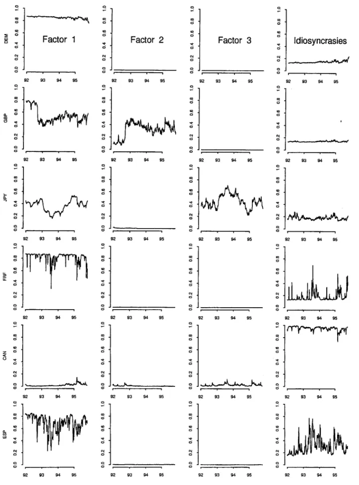
Graphical summaries are presented in Figures 2 to 4. Figure 2 shows the posterior means for the factor loadings through time, while Figure 3 presents the posterior means for the common factors itself and their standard deviations. Finally, Figure 4 present the proportion of the time series variances explained by each of the factors, common and specific. Before considering the potential sequential benefits of these mo deIs , a few interesting general comments are appropriate. To begin with, allowing the idiosyncratic variances to follow stochastic volatility models has little or impact on the point estimates for most of the parameters. Apart from some of the entries in

f3

_{t ,}most of the quantities of interest remains virtually at the same estimates. Secondly, the extended model just exarcebates our previous comment about the necessity of fewer common factors. Previously, a common factor that represented only one the variables could be understood as a adaptation of the model to allow some of the series to have specific variances that varied with time. Now, however, byallowing the specific variances of the series to follow independent stochastic volatility models, we force the factors to fully represent real interactions (possibly dynamic) between the time series at hand.

(7)

The previous comment is exacerbated when comparing Figure 4 to its counterpart ob-tained when fitting our new model with static idiosyncratic variances. The proportion of the variance explained by the first common factor is virtually unchanged, the same being said about the second common factor. The third factor is the one that sheds more light on our previous comments. For instance, in the simpler model the variability of the Japanese currency was explained by the first common factor (40%), the third common factor (40%), and by its idiosyncratic factor (20%), for most of the time período In our new model, all the weight attributed to the third factor is relocated to its specific factor, indicating that, in fact, the third factor is unimportant. The Spanish Peseta has a similar behaviour too.

Following the previous discussion we have considered a one and two-factor model. In the one-factor model, the posterior distríbution for the parameters defining the factor stochastic volatility are such that: E(a) = -9.904, SD(a) = 0.313, E(</» = 0.9891,SD(</» = 0.0057

and E(U) = 0.0037, SD(U) = 0.0015. Also, the following exhibit shows point estimates

(posterior means) for

f3

_tfor

t

=

1,500,1000

t = l t = 500 t = 1000 1.00

0.84

l3t=

0.46

0.96 0.05 0.93

for the one-factor model and,

1.00 0.74 0.55 0.96 -0.04 0.92

t

= 500 1.00 0.00 0.73 1.00 0.54 0.00 0.96 0.03 t = l

1.00 0.00 0.73 1.00 0.41 0.32 0.96 0.03 0.03 0.12 0.91 0.15

-0.05 0.04 0.92 0.06

1.00 0.65 0.69 0.96 -0.10 0.90

t

=

1000 1.00 0.00 0.73 1.00 0.67 -0.11 0.96 0.03 -0.10 0.01 0.90 0.08

for the two-factor model. As we expected, the time seríes variances explained by the second and third factors moves to the idiosyncratic components in the one-factor model. The second and third factors are basically responsible for part of the variances of GBP and JPY, respectively, and are those two currencies that have their idiosyncratic variances changed as the number of factors is decreased from three to one. Changes on DEM, FRF, CAN and JPY's idiosyncratic variances are immaterial, suggesting that an one-factor model is enough to explain the co-movements in those currencies. We will discuss further this issue later on in the next chapter when conducting sequential predictive and portfolio comparisons amongst alternative models.

(8)

4 Conclusions

We extended the existing factor stochastic volatility models by allowong the loadings matrix to evolve over time and capture structural changes in the market conditions. In order to perform estimation and forecasting in the generalized models, new MOMO algorithms were proposed and customized. A summary of our most interesting finding follow:

• One of the most important empirical results, we believe, is the relationship between the number of factors, and therefore, common stochastic variances, and whether or not the idiosyncratic variances are modeled by stochastic volatility models. We have found the rather intuitive result that more factors are necessary when the idiosyncratic variances does not follow stochastic volatility models. Those extra factors basically influenced just one of the time series involved in the analysis, therefore using the factor model without its most appealing characteristic, which is to explain co-movements between the time series.

• AIso related to the previous comment is the fact that an indeterminacy may occur when one of the common factors influences just one of the time series and the idiosyncratic variances follow stochastic volatility processes. In this case it is impossible to identify in the likelihood which term is the common factor and which is the idiosyncratic factor and the posterior distribution of the parameters related to those processes are bound to exhibit multimodality. Possible solutions are to restrict the prior distributions to avoid such indeterminacy and assign higher prior probability to models with lower number of common factors.

• More complex structures for the factor loadings, such as higher order auto-regressions, are possible extensions of the models we have studied. AIso, the loadings discount factor, which plays an important role in the estimation process, deserves more atten-tion. For instance, replacing the discount factor by a constant variance matrix for the factor loadings would be an alternative solution, even though the discount factor has a natural appeal in expressing the amount of information retained by the model through time.

• Finally, the structure of the models presented here opens the possibility for on-line estimates and sequential updates of their posterior distributions. This challenging problem represents the most appealing application of these models since it will deliver on-line estimates of the predictive distribution that will help on the decision making processo

Bibliography

Aguilar, O. and West, M. (2000) Bayesian dynamic factor mo deIs and variance matrix discounting for portfolio allocation. Journal of Business and Economic Statistics (June

(9)

Bartholomew, D.J. (1995) Spearman and the origin and development of factor models.

British Journal of Mathematical and Statistical Psychology, 48, 211-220.

Diebold, F. X. and Nerlove, M. (1989) The dynamics of exchange rate volatility: A

multi-variate latent factor ARCH model. Journal of Applied Econometrics, 4, 1-21.

Engle, R. (1987) Multivarite ARCH with factor structures - cointegration in variance. Technical Report. University of California at San Diego.

Geweke, J.F. and Zhou, G. (1996) Measuring the pricing error of the arbitrage pricing

theory. The Review of Financial Studies, 9, 557-587.

Giakoumatos, S.G., Dellaportas, P. and D.D., Politis (1999) Bayesian analysis of some multivariate time-varying volatility models. Technical Report. Department of Statistics, Athens University of Economics and Business, Greece.

Harvey, A.C., Ruiz, E. and Shephard, N. (1994) Multivariate stochastic variance models.

Review of Economic Studies, 61, 247-264.

Jacquier, E., Polson, N.G. and Rossi, P. (1995) Models and priors for multivariate stochastic

volatility. Discussion Paper. Graduate School of Business, University of Chicago. '

Kim, S.N., Shephard, N. and Chib, S. (1998) Stochastic volatility: likelihood inference and

comparison with ARCH models. Review of Economic Studies, 65, 361-393.

Lopes, H. (2000) Bayesian analysis in latent factor and longitudinal models. Ph.D. Thesis. Duke University.

Pitt, M.K. and Shephard, N. (1999) Time varying covariances: A factor stochastic volatility

approach (with discussion). In Bayesian statistics 6 (eds J.M. Bernardo, J.O. Berger, A.P.

Dawid and A.F.M. Smith), pp. 547-570. London: Oxford University Press.

Sentana, E. (1998) The relation between conditionally heteroskedastic factor models and

factor ARCH models. Econometrics Journal, 1, 1-9.

Shephard, N. (1996) Statistical aspects of ARCH and stochastic volatility. In Time Series

Models in Econometrics, Finance and Other Fields (eds D.R. Cox, D.V. Hinkley and O.E.

Barndorff-Nielsen). London: Chapman and Hall.

West, M. and Harrison, P.J. (1997) Bayesian Forecasting and Dynamic Model. New York:

(10)

t

DEM GBP JPY

FRF

CAD

ESP

1 2.41 1.49 0.25 2.87 -1.81 2.06 100 2.48 1.50 0.32 2.87 -1.82 1.70 300 2.62 1.50 0.43 2.85 -1.38 1.53 500 2.68 1.50 0.37 2.84 -1.18 1.48 700 2.76 1.49 0.31 2.83 -0.55 1.58 900 2.76 1.48 0.23 2.84 -0.20 1.58 1000 2.77 1.48 0.20 2.84 -0.19 1.56

Table 1: Three-factor model: retrospecti ve posterior means for t9t ( x 10-4 ),

t

-1,100,300,500,700,900 and 1000 when the idiosyncrasies have stochastic volatility struc-tures (1/1/1992 to 10/31/1995)

t

DEM GBP JPY

FRF

CAD

ESP

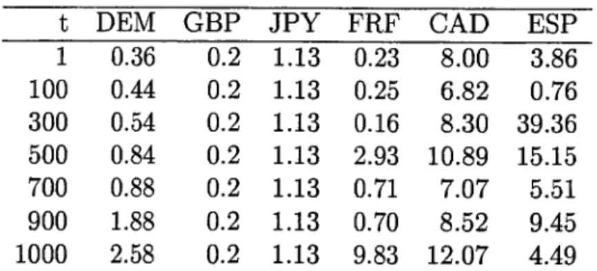
1 0.36 0.2 1.13 0.23 8.00 3.86 100 0.44 0.2 1.13 0.25 6.82 0.76 300 0.54 0.2 1.13 0.16 8.30 39.36 500 0.84 0.2 1.13 2.93 10.89 15.15 700 0.88 0.2 1.13 0.71 7.07 5.51 900 1.88 0.2 1.13 0.70 8.52 9.45 1000 2.58 0.2 1.13 9.83 12.07 4.49

Table 2: Three-factor model: retrospective posterior means for 0"[(x10-6₎_{when the}

idiosyn-crasies have stochastic volatility structures (1/1/1992 to 10/31/1995).

1 -10.191(0.376) 2 -11.828(1.351) 3 -10.942(0.866)

0.978(0.008) 0.991(0.004) 0.988(0.005)

0.053(0.015) 0.076(0.020) 0.115(0.030)

u

0.990(0.005)

0.060(0.016) 0.089(0.023)

0.990(0.008) 0.994(0.004)

0.078(0.024)

Table 3: Three-factor model: retrospective posterior means and standard deviations (in parenthesis) for the stochastic volatility parameters when the idiosyncrasies have stochastic volatility structures . The upper diagonal entries for U represent correlations (1/1/1992 to

(11)

1 ci_i _Pi _Si 1 -13.665(1.507) 0.999(0.001) 0.001(0.000) 2 -15.446(0.212) 0.843(0.105) 0.000(0.000) 3 -13.758(0.323) 0.879(0.093) 0.000(0.000) 4 -14.351(0.411) 0.922(0.023) 0.648(0.181) 5 -11.651(0.190) 0.992(0.005) 0.001(0.000) 6 -11.967(0.248) 0.937(0.020) 0.201(0.061)

Table 4: Three-factor model: retrospective posterior means and standard deviations (in parenthesis) for the stochastic volatility parameters when the idiosyncrasies have stochastic volatility structures (1/1/1992 to 10/31/1995).

92 93 94 95 92 93 94 95

DEM GBP

: 1

92 93 94 95 92 93 94 95

JPY FRF

: 1

92 93 94 95 92 93 94 95

CAD ESP

(12)

(13)

92 93 94 Firstfaclor

92 93 94

Second iactor

92 93 94

Third tactor

95

'"

o

92 93 94 95

First faclor's slancfard deviBlion

92 93 94 95

second factor's standard deviation

92 93 94 95

Third factors standard deviation

Figure 3: Retrospective posterior means for the common factors,

J

t, and their standard

deviations (x 100), the square root of the diagonal elements of Ht, when the idiosyncrasies

(14)

o '"

~

:: .,; '" .,; o .,; co .,; o .,; '" .,; o .,; co .,; '"

z .,;

(j "":

o

'"

.,;

Factor 1

92 93 94 95

â~

~

92 93 94 95

:~

.,; .,. .,; '" .,; o .,;

92 93 94 95

co .,; '" .,;

..

.,; '" .,; o .,; o o co .,; '" .,;

..

o '" .,;

Factor 2

92 93 94 95

â ;:::~

==:;:=::::::;::=:;---co

o

'" o

..

o

'" .,;

92 93 94 95

..

.,; '" o

..

.,; '" .,; o .,; co .,;

Factor 3

92 93 94 95

=~

.,; '" .,; o .,; o co .,; '" .,;

..

o

'" .,; o .,; co o '" .,;

..

o '" .,;

92 93 94 95

o~

.,;

92 93 94 95

..

.,; '" o .,. o '" o o .,;

..

o

'" o

'" .,; o o co o "' o .,. o o o co o Idiosyncrasies

___

-_w ...

~

92 93 94 95

=wlJJ

.,; '" o o o '" o .,. o '" o o o o co

92 93 94 95

:~

o

..

o '" o o o

92 93 94 95

Figure 4: Proportion of the time series variances explained by each of the factors

(15)