Numerical investigation of diffuse instability in sandy soil using
discrete element method under proportional strain path loading
Abstract
The Loose sandy soil can manifest static liquefaction phenomenon under un-drained condition, in which the onset of instability is within the failure line, and there is no obvious shear band. This type of failure mode, very different from localized instability that occurs in dense sand, is called the diffuse instability. In this paper, a series of proportional strain tests and fully drained tests under dif-ferent initial void ratio were simulated using the discrete element method. The influence of strain increment ratio and the initial void ratio affecting the insta-bility of sandy soil were discussed in detail. The development mechanism of pore water pressure in proportional strain tests was analyzed by comparing with the volumetric curve of fully drained test. Finally, a unified mechanism of dif-fuse instability of sandy soil in proportional strain tests was explained. Numeri-cal results indicate that the strain increment ratio and the initial void ratio work together affecting the instability of specimen. The occurrence of diffuse insta-bility is the result of effective stress reduction due to the development of pore water pressure, which depends on the difference of volumetric strain between fully drained tests and proportional strain tests. The increment of pore water pressure is determined by the difference of strain increment ratio, which can be used as an index to reflect the liquefaction potential of sandy soil.
Keywords
Sandy soil; Proportional strain path; diffuse instability; discrete element method.
1 INTRODUCTION
The instability of soil can be considered as a stress state that is reached before the failure line from mechanical per-spective. Any small stress increment under this state will lead to a large plastic strain. Soil instability can be roughly divided into two types: internal instability and external instability (Goddard, 2003). Internal instability refers to the loss of the inherent strength of the soil, and the external instability means that the interaction between the soil and the sur-rounding environment is beyond the bearing limit. The internal instability including localized instability with shear bands and diffuse instability without shear bands. The differences between these two types of instability are discussed in detail by Lade, 1990 and Lancelot et al. (2004). This paper mainly discussed the diffuse instability. The traditional idea holds that soil will not unstable before the effective stress reaches the failure line. But Castro (1969) found that loose sand may manifest liquefaction phenomenon under undrained condition without obvious shear band and the onset of instability is within the failure line. Instability of liquefaction is one of the major reasons which results in the failure of earth structures such as dam. “Liquefaction” is used for the first time by Hazen (1920), describing the failure of the Ca-laveras dam’s failure. Casagrande defined the critical void ratio (CVR) concept in his early paper. Seed and Lee (1966) proposed the concept of “initial liquefaction” and Casagrande (1975) proposed the concept “steady state strength”, which is used to estimate sand liquefaction failure. Later several concepts such as “steady state line”, “flow structure” were proposed to describe the liquefied deformation mechanism by several researchers (Poulos, 1982; Poulos et al, 1985; Prevost,1985; Lade and Pradel, 1990; Bazier and Dobry,1995). More recently, other researchers have carried out exper-imental research of the instability of sand under undrained conditions (Laouafa and Darve, 2002; Daouadji et al, 2009; Daouadji et al, 2011) and developed corresponding constitutive models to explain and predict this type of instability (Mr óz and Boukpeti, 2003; Desai et al, 2005; Rahman et al, 2014; Najma and Latifi, 2017; Chandrakant and Desai, 2016; Liu et al, 2016). These studies provide an important theoretical basis for the analysis of diffuse instability.
In recent years, some studies have shown that diffuse instability can occurs under fully drained conditions (Eck-ersley, 1990, Olson et al., 2000). Therefore, the research on the instability mechanism of soil under different drainage conditions has attracted the attention of many scholars (Sasitharan et al., 1993; Anderson and Riemer, 1995; Chu et al.,
Meng Fana Yang Liua* Jianqiu Hanb Kai Yangb
a Department of Civil Engineering, University of
Science and Technology, Beijing, 100083, China. E-mail: [email protected],
b. Power China Road Bridge Group Co., Ltd.
E-mail: [email protected], [email protected]
*Corresponding author
http://dx.doi.org/10.1590/1679-78255240
e
α− plane was obtained. Furthermore, a unified mechanism of diffuse instability of sandy soil in proportional strain tests is explored by analyzing the development of pore water pressure.
2 NUMERICAL MODEL AND LOADING CONTROL
2.1 NUMERICAL MODEL
The numerical model was established by the three-dimensional discrete element program PFC3D, as shown in Fig-ure 1. Ni et al. (2000) found that increasing the number of particles beyond 15,000 in a 3D DEM simulation raised the computational expense with a relatively small effect on the model results. In addition, according to Wang and Li (2014), who compared the results obtained with 1000, 5000, 10,000, and 20,000 particles, there is no significant difference be-tween the results obtained with 5000, 10,000, and 20,000 particles. In this study, we choose approximate 5000 particles to conduct simulation, which changes with the initial void ratio. The minimum and maximum particle diameters are 1.0 and 1.8mm, respectively, with a mean particle diameter of 1.4mm.
Different sizes of samples were used in previous DEM simulations or laboratory test but the ratio of height to diam-eter is usually taken as about 2.0. For example, the DEM specimen used by Tang (Tang et al., 2016) has a cylindrical structure with the height of 80.5 mm and the diameter of 38 mm; The triaxial specimen tested by Vaid and Eliadorani (1998) is 126 mm height × 63 mm diameter; The triaxial specimen used by Sivathayalan and Logeswaran (2008), is 125 mm height × 63 mm diameter. Therefore, we choose 2.0 as the ratio of height to diameter, to build numerical model. Then the appropriate diameter of 16 mm can be obtained ( 3
4π×0.7 ×5000 / 3 16≈ ). We choose 20mm as the sample diameter and the height is 40mm considering the influence of initial porosity of the assembly.
Figure 1: Typical numerical sample.
2.2 CALIBRATION OF PARAMETERS AND VERIFICATION WITH TYPICAL EXPERIMENTAL RESUTLS
The linear contact model was adopted here and three micromechanical parameters, i.e, normal contact stiffness kn,
contact stiffness ratio kn/ks and inter-particle friction
µ
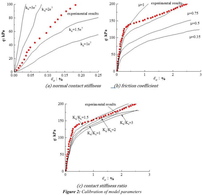
are to be determined. Usually, the normal contact stiffness knWe tried five kn values to conduct a series of simulations with empirical values of µ=0.5 and kn/ks=1.0. The
simula-tion results were compared with the experimental data, as shown in Figure 2. The initial slopes of the stress-strain curve (initial stiffness) were compared with the simulating results from DEM. One can see from Figure 2 that the numerical result of kn=1.5×10⁷ N/m is best fit for the initial stiffness of stress-strain curve, which is then be chosen as the
simula-tion parameters.
After that, we tried four friction coefficient values to conduct simulations with kn=1.5e7 and kn/ks=1.0. The
simula-tion results were compared with the experimental data again, as shown in Figure 3. One can see that the numerical result of µ=0.75 is most consistent with the peak strength of sample. Finally, we adjusted the values of contact stiffness ratio kn/ks to fit experimental results, as shown in Figure 4, and the value of kn/ks=1.5 is then be determined.
Figure 2: Calibration of model parameters
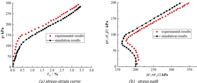
Simulation was then carried out using the selected parameters calibrated from fully undrained test. A typical exper-iment under partial drainage condition (α =0.1) were selected to assess preliminarily the ability of the developed DEM model and acceptability of chosen parameters. Figure 3 shows the comparison of simulation results with experimental results. One can see from Figure 3 the simulated macro-response from DEM has a good agreement with the results of laboratory tests.
Figure 3: Results verification with the experimental results. under partial drainage condition α=0.1
2.3 NUMERICAL SIMULATION SCHEME
The loading program is described by the following conditions for the imposed proportional strain test:
1 0
dε > (1)
2 3
dε =dε (2)
1 v
d d
α = ε ε (3)
where dε1, dε3is the increment of axial strain and radial strain respectively; dεv is the increment of volumetric strain. Using the common sign convention used in geomechanics, axial compression and volume outflow are considered as positive. Therefore, a positive α value corresponds to volumetric contraction and a negative α value corresponds to volumetric expansion. Depending on the value and sign of the parameter α the test can be classified into three types: (1)
α
=0 represents undrained test; (2)α
>0 corresponds to contractive test; (3)α
<0 means expansive test.It should be noticed that α =1 corresponds to a one-dimensional test. Although the in-situ conditions are clearly dif-ferent, a constant strain ratio has been chosen for the whole test to study the influence of drainage condition on the insta-bility of sands.
A total of 14 samples with different initial void ratio were selected. The void ratio range is: 0.618~0.98. The mini-mum and maximini-mum strain increment ratio α are -0.5 and 0.5, respectively, with interval value of 0.05. Therefore 21×
14 proportional strain tests were simulated in all. The simulation scheme is shown in table 1.
Table 1: Numerical simulation scheme
e
α 0.618 0.658 0.715 0.748 0.754 0.767 0.779 0.818 0.838 0.862 0.89 0.9 0.912 0.98 -0.5 0.5 A1-U1 A2-U2 A3-U3 A4-U4 A5-U5 A6-U6 A7-U7 A8-U8 A9-U9 A10-U10 A11-U11 A12-U12 A13-U13 A14-U14
3 DIFFUSE INSTABILITY
3.1 DIFFUSE INSTABILITY IN UNDRAINED TESTS (
α
=0)One of the key points to study the diffuse instability is how to determine the instability point. According to Chang et al. (2010), the instability conditions can be divided into two modes:
Mode 1: If the determinant of stiffness matrix is zero. In this case, the sample bifurcates with the occurrence of un-limited displacement rates, which is considered as the onset of localization.
Mode 2: Loss of positiveness of second-order work. In this case, the second-order work could become zero while the determinant of stiffness matrix remains positive.
The diffuse instability belongs to Mode 2 failure. Hill’s second-order work criterion has been widely applied to judge the stability of granular materials (Sibille et al., 2015; Hadda et al., 2015; Darve and Laouafa, 2015; Darve et al., 2004; Nicot et al., 2010; Daouadji et al., 2010; Sawicki and Świdziński, 2010). which states that a material, progressing from one stress state to another, is stable if the second-order work is strictly positive. For triaxial conditions, it can be written as following:
2 '
1 3 v
d w=dqdε +dσ εd (4)
Where ' 1
σ = axial effective stress; ' 3
σ = radial effective stress; ε1= axial strain; ε3= radial strain;
q
=
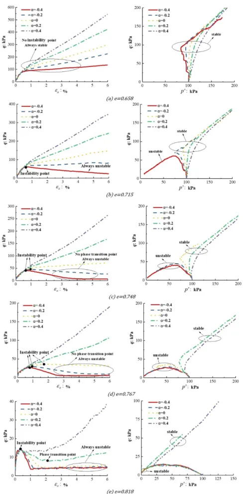
deviatoric stress; and εv = volumetric strain.The results of undrained tests with various initial void ratios are presented in Fig. 4. Corresponding test number is K2, K3, K4, K6, K8. As indicated in Fig. 4(a), For dense sand (e=0.658, e=0.715, e=0.748), the deviatoric stress contin-uously increases, and no maximum peak strength can be observed. For medium-dense sand (e=0.767), the deviatoric stress first reaches a peak, then decreases slightly but finally the strength is recovered. For loose sand (e=0.818), The peak value of deviatoric stress is reached rapidly, which is followed by a rapid decrease of the deviatoric stress down to a minimum strength. The minimum strength can be almost zero for loose sands, which represents the phenomenon called static liquefaction.
during the undrained test dεv =0, the second-order work is therefore given by:
2
1
d w=dqdε (5)
As the axial strain is increased, equation (5) vanishes only if dq=0. The deviatoric stress
q
becomes the control parameter and the peak value of deviatoric stress corresponds to the instability point. The second-order work is computed by equation (5) and plotted in Fig. 5 against the axial strain.It is seen that, for the three dense samples of e=0.658, e=0.715 and e=0.748, the value of second-order work always keeps positive, so it is always in a stable state. The second-order work of the e=0.767 sample drops to a negative value near the strain of 1.4% and then rises to a positive value near the strain of 7.2%. This phenomenon is called partial fail-ure and the stress state of ε1=7.2% is called the phase transition point. For the loose sample of e=0.818, the value of second-order work is always negative after the instability point, so there is no phase transition point, and it is always in unstable state after the instability point. From Fig. 4(b) we can see that the instability lines are within the critical state line, which indicate that the type of instability occurred in these three samples belongs to the diffuse instability.
Figure 4: Simulated results of proportional strain test for α =0: (a) stress-strain curve; (b) stress path.
0 2 4 6 8 10 12
-10 0 10 20 30
40 e=0.658
e=0.715 e=0.748 e=0.767 e=0.818
Instablity point phase transition point
d
2 w
:P
a
%
Figure 5: Second-order work curves of proportional strain test forα =0.
3.2 DIFFUSE INSTABILITY VARIED WITH THE INITIAL VOID RATIO
To study the influence of initial void ratio on soil instability in other drainage conditions (
α
>0 orα
<0). We choose a series of proportional strain tests under different α value with the same 5 initial void ratio samples to analyze. For the sake of clarity, only the results ofα
=0.5 andα
= −0.5 proportional tests are analyzed here, corresponding test numbers are A2, A3, A4, A6, A8 and U2, U3, U4, U6, U8. The simulation results of proportional tests under other αvalues are similar.
Figure 6: Simulated results of proportional strain test for α =0.5: (a) stress-strain curve; (b) stress path.
Figure 7: Simulated results of proportional strain test forα = −0.5: (a) stress-strain curve; (b) stress path.
3.3 DIFFUSE INSTABILITY VARIED WITH THE
α
VALUEFigure 8 shows the results of different α values under the same void ratio. For clarity, only five α values of 0.4, 0.2, 0, -0.2 and -0.4 are drawn here. Although the dense sample of e=0.715 remains stable under
α
=0 condition, it is unstable when0.4
α
= − . While the loose sample of e=0.818 is unstable whenα
=0, it becomes stable underα
=0.4 conditions. For the dense sample of e=0.658, there is no strain softening phenomenon can be observed even underα
= −0.4 condition, but it canbe foreseen that the sample will eventually lose its stability with the further reduction of α value. Obviously, under the same confining pressure, whatever the void ratio is, the sample with the smaller α value is more prone to instability. Therefore, the
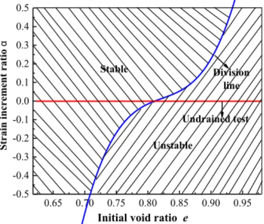
3.4 DIFFUSE INSTABILITY REGIONAL MAP IN
α
−
e
PLANEIt should be emphasized that during the proportional tests with α ≠0, the deviatoric stress
q
will not be the control parameter any more. Substituting equation (3) into equation (4) yields the following equation:(
)
2 ' '
1 3 1 3 1
d w=dqd
ε
+dσ α ε
d =d q+ασ
dε
(6)Therefore, the control parameter changes from deviatoric stress
q
to ' 3q+ασ . However, dq<0 is still a necessary condition for the onset of diffuse instability, for the convenience of discussion, we use dq<0 as collapse criteria for all proportional tests. Since the strength will finally be recovered in partial failure, only the second type of diffuse instability are discussed in this paper.
The stable/unstable regional map of all proportional tests in α−e plane is drawn as shown in Figure 9. The graph is divided into two parts by undrained tests: the upper part is volume contraction area and the lower part is volume dilata-tion area. We take the simuladilata-tion results from samples of e=0.767 as example to explain the stable/unstable regional map. There is no phase transition point after instability point when α = -0.4, -0.2 and 0 for sample of e=0.767. Therefore, the coordinate pairs of (0.767, -0.4), (0.767, -0.2) and (0.767, 0) related to unstable responses are contained in unstable re-gion. However, the deviatoric stress continuously increases and no peak strength can be observed when α = 0.2 and 0.4. Therefore, the coordinate pairs of (0.767, 0.2), (0.767, 0.4) related to stable responses will be contained in stable region.
One can see from Figure 9 that some dense samples keep stable under undrained condition but become unstable in the volume dilatation area. On the contrary, some loose samples are unstable under undrained condition, but remain sta-ble in the volume contraction area. The left side of the division line is close to negative infinity and the right side goes to positive infinity, which represents very dense sand (rock) and extremely loose sand(mud). This is only an idealization, which already has no properties of sand.
In general, the value of α and initial void ratio affect the instability of sand in two aspects under the same confin-ing pressure. Each proportional test is a specific combination of α and e, and whatever the void ratio is, there is always a α value to make it unstable. Therefore, no matter what density of sand is, it is possible to lose stability if the drainage condition is suitable, and the looser sand is more prone to instability regardless of the drainage condition.
0.65 0.70 0.75 0.80 0.85 0.90 0.95 -0.5 -0.4 -0.3 -0.2 -0.1 0.0 0.1 0.2 0.3 0.4 0.5 St r a in inc r e m e nt r a tio α
Initial void ratio e
Unstable
Undrained test Division line Stable
Figure 9: Stable / unstable region obtained from simulations results
4 MECHANISM OF DIFFUSE INSTABILITY ASSOCIATED WITH THE DEVELOPMENT PORE WATER PRESSURE
4.1 PORE WATER PRESSURE FORMULA
The calculation of pore water pressure in the discrete element model adopts the equivalent principle, that is, the to-tal confining pressure is assumed to be constant. According to the effective stress theory, the sum of the increment of pore water pressure and the increment of effective confining pressure equals 0. This implies:
' '
3 u 3 0 u 3
σ σ σ
∆ + ∆ = ∆ = ⇒ ∆ = −∆ (7)
where ' 3
σ
∆ = increment of effective confining pressure; ∆ =u increment of pore water pressure; ∆σ3= increment of total confining pressure.
d p
v v v
ε ε ε
∆ = − (9)
where d v
ε = volumetric strain of fully drained test; p v
ε = volumetric strain of proportional strain test.
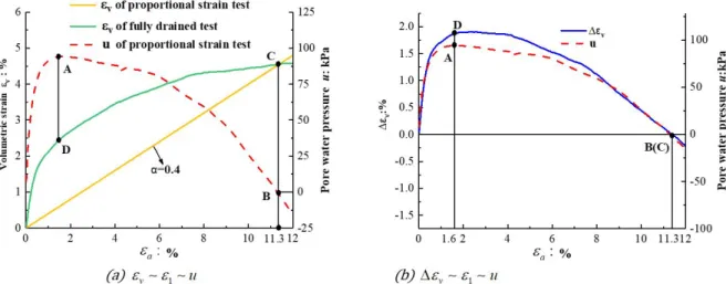
We chose the simulation results of e=0.838 sample with
α
=0.4 as an example to analyze, and the results of otherα values are similar. Fig. 10 shows correlation between pore-water pressure curve and volumetric strain curve for e=0.838 sample. The point A represents peak value of pore water pressure. The point C is the intersection point of volu-metric strain curve for fully drained test and proportional strain test (∆εv =0). Before the point C ∆εv >0, after the point C ∆εv<0. The point B is the zero point of pore-water pressure curve. Before the point B u>0, after the point B
0
u< .
As shown in Figure 10 (a), point B and point C are approximately at the same strain level (εa=11.3%), which im-plies that point C correspond to the zero point of pore pressure. In other words, when the accumulative volumetric strain of the proportional strain test is equal to the accumulative volumetric strain of fully drained test, the accumulative pore water pressure will be equal to zero. Taking the BC line as a boundary we can see that ∆εv >0 corresponds to u>0 and
0 v
ε
∆ < corresponds to u<0. Obviously, the value of the accumulative pore water pressure of proportional strain test depends on the value of ∆εv. To analyze the results of other α values also have the same rule, here are not to be dis-cussed in detail due to limited space.
It can be noticed from Fig. 10 (b) that the value of ∆εv reaches maximum at point D, which indicate that the strain increment ratio of two tests are equal (=0.5). The strain increment ratio (equation 4) essentially implies the development of the dilatancy during the loading of the soil. To further analyze the relationship between pore water pressure and the dilatancy of soil, we define ∆
α
as follows:d p
α α α
∆ = − (10)
Where α =d
strain increment ratio in fully drained test; α =p
strain increment ratio in proportional strain test.
Fig. 11 shows correlation between pore-water pressure and the strain increment ratio during loading for e=0.838 sample. The point A and point C in the diagram are still the peak and zero point of the pore water pressure curve, and the point D is the intersection point of the strain increment ratio of two tests. Before the point D ∆ >
α
0, which will makev
ε
∆ increase. After the point D ∆ <
α
0, which will make ∆εv decrease. Therefore, the point D corresponds to the peak value of ∆εv and pore water pressure, which is point A. Similar relationship can be obtained if we take AD line as a boundary, which is ∆ >α
0 corresponds to ∆ >u 0 and ∆ <α
0 corresponds to ∆ <u 0.In summary, the accumulative pore water pressure in proportional strain test depends on the value of ∆εv, and the increment of pore water pressure depends on the value of ∆
α
.Figure 11: Correlation between pore-water pressure and strain increment ratio during loading for sample with e=0.838.
4.3 THE EFFECT OF
α
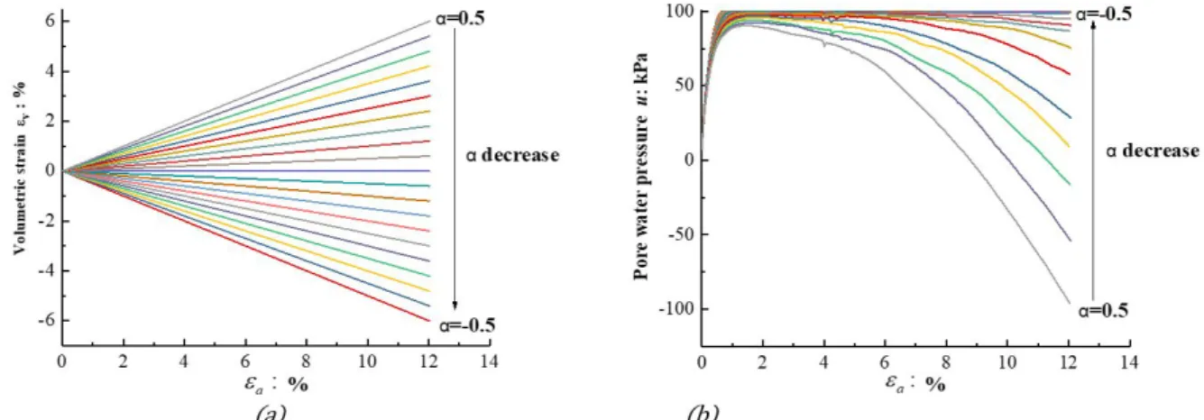
VALUE AND INITIAL VOID RATIO ON THE DILATANCYFig. 12 (a) gives the volumetric strain curves in proportional strain tests with different α value. The volumetric strain curve gradually increases with the increase of α value. It is well known that loose sand has contraction property and dense sand has dilatation property during fully drained loading. As mentioned earlier, a positive εv (or α ) value corresponds to volumetric contraction and a negative εv (or α ) value corresponds to volumetric expansion, therefore the volumetric strain curve of fully drained test will gradually decrease with the increase of initial void ratio.
Figure 12: (a) Volumetric strain curve of proportional strain tests with different α value; (b) Pore water pressure curve for proportional strain tests with different α value (e=0.838 sample).
(1) In the proportional strain test, the strain increment ratio α and the initial void ratio e work together to affect the instability of specimen. No matter what the initial density of the sample is, it may be unstable if the drainage condition is suitable. Meanwhile, under the same drainage conditions, loose samples are more prone to instability. At a given confining pressure, there is a destabilizing boundary line in α−e plane.
(2) The occurrence of diffuse instability is the result of effective stress reduction due to the development of pore water pressure. The accumulated pore water pressure depends on the value of ∆εv and the increment of pore water pressure is determined by the
value of∆
α
.(3) The actual in situ drainage conditions will be neither fully drained nor fully undrained, and the imposed constant increment strain ratio is also impossible. However, the value of ∆εvand ∆
α
provide an elegant framework to understand how a soil can liquefy despitedrainage conditions. The development of ∆εv and ∆
α
are needed to be analyzed when investigating the instability mechanismof sand and the values of∆
α
(or ∆εv) can be used as an index to reflect the liquefaction potential of sandy soil.Acknowledgements
Authors appreciate the financial support of Beijing Excellent Talent Training Program (2013D009006000005) and the support of Science and technology project of PowerChina RoadBridge Group Co., Ltd.
References
Anderson, S.A., Riemer, M.F., (1995). Collapse of saturated soil due to reduction in confinement. Journal of Geotech-nical Engineering 121(2): 220-261.
Alipour, M.J., Lashkari, A., (2018). Sand instability under constant shear drained stress path. International Journal of Solids & Structures.
Bazier M.H, Dobry R., (1995). Residual strength and large deformation potential of loose silty sands. Journal of Ge-otechnical Engineering Division, ASCE, 121(12):896-906.
Castro, G., (1969). Liquefaction of sands, Harvard Soil Mechanics Series (81).
Casagrande A. (1975). Liquefaction and cyclic deformation of sands-a critical review. Pro of the Fifth Pan American Conf on Soil Mechanics and Foundation Engineering, Buens Aires, Argitina,
Chang, C. S., Yin, Z. Y., & Hicher, P. Y. (2010). Micromechanical analysis for interparticle and assembly instability of sand. Journal of Engineering Mechanics, 137(3), 155-168.
Chu, J., Lo, S.R., Lee, I.K., (1992). Strain-Softening Behavior of Granular Soil in Strain-Path Testing. Journal of Ge-otechnical Engineering 118(2):191-208
Chu, J., Lo, S.R., Lee, I.K., (1993). Instability of granular soils under strain path testing. Journal of Geotechnical Engi-neering 119(5): 874-892.
Chandrakant, Desai, C. S. (2016). Disturbed state concept as unified constitutive modeling approach. Journal of Rock Mechanics and Geotechnical Engineering, 8(3): 277-293.
Daouadji, A., Algali, H., Darve, F., (2009). Instability in Granular Materials: Experimental Evidence of Diffuse Mode of Failure for Loose Sands. Journal of Engineering Mechanic 136(5):575-588.
Daouadji, A., Darve, F., Gali, H.A., (2011). Diffuse failure in geomaterials: Experiments, theory and modelling. Interna-tional Journal for Numerical & Analytical Methods in Geomechanics 35(16):1731–1773.
Desai, C.S., Pradhan, S.K., Cohen, D., (2005). Cyclic Testing and constitutive modeling of saturated sand–concrete in-terfaces using the disturbed state concept. International Journal of Geomechanics 5(4): 286-294.
Dong, Q., Xu, C., Cai, Y., (2016). Drained instability in loose granular material. International Journal of Geomechanics 16(2).
Daouadji, A., Hicher, P. Y., Jrad, M., Sukumaran, B., & Belouettar, S. (2013). Experimental and numerical investigation of diffuse instability in granular materials using a microstructural model under various loading paths. Geotechnique, 63(5), 368-381.
Darve, F., Laouafa, F., (2015). Instabilities in granular materials and application to landslides. International Journal for Numerical and Analytical Methods in Geomechanics 5(8):627-652.
Darve, F., Servant, G., Laouafa, F., (2004). Failure in geomaterials: continuous and discrete analyses. Computer Methods in Applied Mechanics and Engineering 193(27):3057-3085.
Daouadji, A., Algali, h., Darve, F., (2010). Instability in granular materials: experimental evidence of diffuse mode of failure for loose sands. Journal of Engineering Mechanics 136(5):575-588.
Eckersley, J.D., (1990). Instrumented laboratory flow slides. Geotechnique 40(3): 489-502.
Goddard, J.D., (2003). Material instability in complex fluids. Annual Review of Fluid Mechanics 35: 113-133.
Gu, X., Huang, M., Qian, J., (2014a). DEM investigation on the evolution of microstructure in granular soils under shearing. Granular Matter 16(1):91-106.
Gu, X., Huang, M., & Qian, J. (2014b). Discrete element modeling of shear band in granular materials. Theoretical & Applied Fracture Mechanics, 72(1), 37-49.
Guo, N., Zhao, J., (2016). 3D multiscale modeling of strain localization in granular media. Computers & Geotechnics 80:360-372.
Hazen, A. Hydraulic fill dams. Transactions, American Society of Civil Engineers, (1920), 83: 1713-1745.
Hill, R., (1958). A general theory of uniqueness and stability in elastic-plastic solids. Journal of the Mechanics and Phys-ics of Solids 6(3): 236-249.
otechnique:1-49.
Liu Y., Chang C.S., Wu S.C. (2016). A Simple One-Scale Constitutive Model for Static Liquefaction of Sand-Silt Mix-tures, Latin American Journal of Solids and Structures 13:2190-2218.
Mróz, Z.N., Boukpeti., (2003). A Drescher Constitutive model for static liquefaction. International Journal of Geome-chanics 3(2):133-144.
Mital, U., Andrade, J.E., (2016). Mechanics of origin of flow liquefaction instability under proportional strain triaxial compression. Acta Geotechnica 72:1-11.
Najma, A., Latifi, M., (2017). Predicting flow liquefaction, a constitutive model approach. Acta Geotechnica 12(4):1-16.
Nicot, F., Daouadji, A., Hadda, N., (2013). Granular media failure along triaxial proportional strain paths. European Journal of Environmental and Civil Engineering 17(9): 777-790.
Nicot, F., Sibille, L., Hicher, P.Y., (2015). Micro–macro analysis of granular material behavior along proportional strain paths. Continuum Mechanics & Thermodynamics 27(1-2):173-193.
Nicot, F., Darve, F., Huynh, D.V.K., (2010). Bifurcation and second-order work in geomaterials. International Journal for Numerical and Analytical Methods in Geomechanics 31(8):1007-1032.
Ni, Q., Powrie, W., Zhang, X., & Harkness, R., (2000). Effect of particle properties on soil behavior: 3-D Numerical Modeling of Shearbox Tests[C]. 96:58-70.
Olson, S.M., Stark, T.D., & Walton, W H. (2000). 1907 Static liquefaction flow failure of the north dike of Wachusett dam. Journal of Geotechnical and Geo-environmental Engineering 126(12): 1184-1193.
Poulos, S.J. (1982). Closure of "the steady state of deformation". Journal of the Geotechnical Engineering Division, 108: 1087-1091.
Poulos, S.J., Castro, G., & France, J.W., (1985). Liquefaction evaluation procedure. Journal of Geotechnical Engineering, 111(6): 772-792.
Prevost, J.H., (1985). A simple plasticity theory for frictional cohesionless soils. International Journal of Soil Dynamics and Earthquake Engineering, 4(1): 9-17.
Sasitharan, S., Robertson, P.K., Sego, D.C., (1993). Collapse behavior of sand. Canadian Geotechnical Journal 30(4): 569-577.
Seed, H.B. and K.L. Lee. (1966) Liquefaction of saturated sands during cyclic loading. ASCE Journal of the Soil Mech. and Found. Eng. Div., 92(6):105-134.
Skopek, P., Morgenstern, N.R., Robertson, P.K., (2011). Collapse of dry sand. Canadian Geotechnical Journal 31(6): 1003-1008.
Sivathayalan, S., & Logeswaran, P., (2008). Experimental assessment of the response of sands under shear–volume cou-pled deformation. Revue Canadienne De Géotechnique, 45(9), 1310-1323.
Sivathayalan, S., & Logeswaran, P., (2007). Behaviour of sands under generalized drainage boundary conditions. Cana-dian Geotechnical Journal, 44(2), 138-150.
Sibille, L., Hadda, N., Nicot, F., (2015). Granular plasticity, a contribution from discrete mechanics. Journal of the Me-chanics and Physics of Solids 75:119–139.
Sawicki, A., Świdziński, W., (2010). Modelling the pre-failure instabilities of sand. Computers and Geotechnics 37(6):781-788.
Tang, H., Zhang, X., & Ji, S. (2016). Discrete element analysis for shear band modes of granular materials in triaxial tests. Particulate Science & Technology, 35(3).
Vaid, Y.P., Eliadorani, A., (1998). Instability and liquefaction of granular soils under undrained and partially drained states. Canadian Geotechnical Journal 35(6):1053-1062.
Wang, X. L., & Li, J.C., (2014). Simulation of triaxial response of granular materials by modified dem.Science China (Physics, Mechanics and Astronomy),57(12), 2297-2308.