Use of generative algorithms and shape optimization strategies in structural design

(1)

Carlos Alberto Ferreira Gomes

Use of generative algorithms and shape

optimization strategies in structural design

Carlos Alberto Ferreira Gomes

Novembro de 2014 UMinho | 201 4 Use of g ener ativ e algor it hms and shape op timization s tr ategies in s tr uctur al design

Universidade do Minho

Escola de Engenharia

(2)

(3)

Novembro de 2014

Dissertação de Mestrado

Ciclo de Estudos Integrados Conducentes ao

Grau de Mestre em Engenharia Civil

Trabalho efetuado sob a orientação do

Professor Doutor Miguel Ângelo Dias Azenha

Arquitecto Filipe Afonso (Arquitectos Anónimos)

Carlos Alberto Ferreira Gomes

Use of generative algorithms and shape

optimization strategies in structural design

Universidade do Minho

Escola de Engenharia

(4)

i

ACKNOWLEDGEMENTS

First of all, I would like to express my deepest gratitude to my advisor, Prof. Miguel Azenha, for all the enthusiasm demonstrated during the course of this thesis, for the knowledge transmitted related to various areas, and above all, for the trust placed in me and consequent opportunities presented which allowed me to grow in a professional and personal level.

I also thank my co-advisor, Arch. Filipe Afonso, for all the contributions given and especially for presenting different perspectives and inspirations whenever needed.

The contribution of the Arch. Nuno Lacerda (CNLL, Lda) and the Arch. Vanessa Tavares (CNLL, Lda) was essential to this work, therefore I am grateful for the time the y both kindly expended which led to valuable feedback to improve this work.

Eng. Nuno Rego (DOKA Portugal) also deserves a special thanks for the availability and transmitted knowledge related to constructability aspects of thin shells structures, that would be much more difficult to obtain without him.

I am also grateful for the support and the vote of confidence deposited by Eng. José C. Lino (Newton) and by the Eng. Eulália Soares (Newton) which undoubtedly increased my commitment.

The knowledge related to computer science patiently transmitted by the Eng. Paulo Rodrigues and the Eng. Rui Barros at the early stages of this dissertation, was also essential to achieve the proposed objectives, for which I am extremely grateful.

I present also my sincere appreciation to all my family and friends who have contributed to my success during my academic life, specially to my Father, Mother and my Sister for all the patience and support.

Lastly, I present my gratitude to Mariana Gomes for all the unconditional support throughout this phase, for all the contributions she gave to this work, and especially for all the affection.

(5)

(6)

iii

ABSTRACT

The aim of this work is to address the challenges and opportunities that are placed at the structural design by the availability of software applications with graphical capabilities able to obtain arbitrary geometries, usually called freeform, and its automatic interoperability with structural analysis tools. The focus of this dissertation is to establish methodologies and interfaces that enable the collaborative and integrated work in real time between Engineers and Architects for the design of freeform structures based in reinforced concrete membranes. In this context, the concepts of formfinding and morphogenesis are discussed and explored. The presented document also describes the implementation and use of a custom made application, developed as part of this dissertation, which enables real-times interoperability between a CAD software and a structural analysis software.

(7)

(8)

v

RESUMO

Pretende-se com este trabalho abordar os desafios e oportunidades que são colocados à conceção estrutural pela disponibilidade de aplicações informáticas com capacidades gráficas capazes de obter geometrias arbitrárias, usualmente designadas por freeform, e sua interoperabilidade automática com ferramentas de análise estrutural. A presente tese tem como enfoque especial o estabelecimento de metodologias e interfaces que permitam o trabalho colaborativo e integrado em tempo real entre Engenheiros e Arquitetos para a conceção de estruturas freeform baseadas em membranas de betão armado. Nesse contexto, são abordados e explorados os conceitos de

formfinding e morfogênese. Este documento descreve ainda a implementação e utilização de uma

aplicação, desenvolvida no âmbito desta tese, que permite a interoperabilidade em tempo real entre uma aplicação CAD e uma aplicação de cálculo estrutural.

(9)

(10)

vii

INDEX OF FIGURES

Figure 1-1 a) National Museum Honestino Guimarães in Brasilia (Inojosa, 2010); b) Tenerife Concert Hall in Tenerife (Lightgruppe Gantenbrink, 2005). ... 1 Figure 1-2 a) Restaurant Los Manantiales in Xochimilco; b) BP Service Station in Deitingen (Garlock & Billington, 2014). ... 2 Figure 2-1 Poleni’s drawing of Hooke’s analogy between an arch and a hanging chain (Block, DeJong, & Ochsendorf, 2006). ... 6 Figure 2-2 Representation of three catenary curves. ... 7 Figure 2-3 a) Schematic representation of St. Peter's Dome; b) Poleni's analysis of St-Peter's Dome (Block, DeJong, & Ochsendorf, 2006) ... 7 Figure 2-4 Three arches' geometry. ... 8 Figure 2-5 Map of vertical displacements for: a) Arch 1 (catenary); b) Arch 2; c) Arch 3. Units in cm. ... 9 Figure 2-6 Map of bending moments for: a) Arch 1 (catenary); b) Arch 2; c) Arch 3. Units in kN/m. ... 9 Figure 2-7 a) Original design for the Colònia Güell (Hensbergen, 2001); b) Colònia Güell's Crypt in 2008 (Canaan, 2008)... 10 Figure 2-8 Hanging model used to define the shape of Colònia Güell: a) uncompleted and created by Gaudi (Huerta, 2006); b) recreated by other artist (Addis, 2014). ... 10 Figure 2-9 a) Sydney Opera House (Utzon, 2002); b) Kresge Auditorium (Bletzinger & Ramm, 2014). ... 11 Figure 2-10 Cross-sectional representation of the two domes: sphere-based and catenary-based.12 Figure 2-11 - Map of vertical displacements: a) spherical dome; b) catenary shaped dome. Units in cm. ... 12 Figure 2-12 Map of membrane forces in the hoop direction: a) spherical dome; b) catenary shaped dome. Units in kN/m. ... 13 Figure 2-13 Map of membrane forces in the meridional direction: a) spherical dome; b) catenary shaped dome. Units in kN/m. ... 13

(15)

xii

Figure 2-14 Hyperboloid Paraboloid with: a) curved boundaries, b) straight boundaries (Holzer,

Garlock, & Prevost, 2008). ... 14

Figure 2-15 Formwork used for the creation of the Chapel (Holzer, Garlock, & Prevost, 2008). 14 Figure 2-16 Félix Candela's Chapel Lomas de Cuernavaca (Holzer, Garlock, & Prevost, 2008). 15 Figure 2-17 Heinz Isler Shell (Borgart & Eigenraam, 2012). ... 15

Figure 2-18 Fibers parallel to the edge and corresponding shape (adapted Bletzinger & Ramm, 2014). ... 16

Figure 2-19 Fibers diagonal to the edge and corresponding shape (adapted Bletzinger & Ramm, 2014). ... 16

Figure 2-20 Shell geometry: a) without the folded edge; b) with the folded edge (Tysmans, 2013). ... 17

Figure 2-21 a) Membrane under pressure (Chilton, 2000); b) full scale structure (Garlock & Billington, 2014). ... 17

Figure 2-22 Soap Film used by Frei Otto (adapted Addis, 2014). ... 18

Figure 2-23 Physical model for static and dynamic load analysis (Tysmans, 2013). ... 18

Figure 2-24 Dutch Maritime Museum in Amsterdam (Adriaenssens, et. al, 2012)... 19

Figure 2-25 Spring- mass-damper system (adapted Adriaenssens, 2014). ... 20

Figure 2-26 Expected graph for: a) node displacement; b) kinetic energy. ... 23

Figure 2-27 Representation of: a) initial shape; b) support conditions. ... 24

Figure 2-28 Results of a system with: a) high stiffness; b) low stiffness. ... 24

Figure 2-29 Mannheim Multihalle by Frei Otto (Verde & Truco, 2009). ... 25

Figure 2-30 Networks of a cables (Basso, et. al, 2009). ... 25

Figure 2-31 Network of linear members... 26

Figure 2-32 Initial shape (Linkwitz, 2014). ... 28

Figure 2-33 Different shape solutions varying the force density value (Linkwitz, 2014). ... 28

Figure 2-34 Particle-Spring System. ... 29

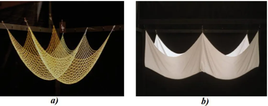
Figure 2-35 Boundary and Support conditions: a) network of chains; b) piece of cloth. ... 31

Figure 2-36 Particle-spring network simulation results for a network of chain. ... 31

Figure 2-37 Particle-spring network simulation results for a piece of cloth. ... 31

Figure 2-38 Map of bending moments in x-direction for the structure obtained by the: a) network of chains; b) piece of cloth. Units in kN.m/m. ... 32

(16)

xiii Figure 2-39 Map of membrane forces in x-direction for the structure obtained by the: a) network

of chains; b) piece of cloth. Units in kN/m... 32

Figure 2-40 Recreated models of: a) hanging chains; b) hanging piece of cloth (Bletzinger & Ramm, 2014). ... 33

Figure 2-41 Concrete structure in: a) Bangalore, India; b) Mexico City, Mexico (Bhooshan, Veenendaal, & Block, 2014). ... 33

Figure 2-42 Landscape: a) empty; b) populated. (Rutten, 2010). ... 35

Figure 2-43 Landscape results from: a) generation 1; b) generation 2. (Rutten, 2010). ... 36

Figure 2-44 Kakamigahara crematorium, Gifu, Japan (Pugnale & Sassone, 2007). ... 37

Figure 2-45 Individuals in the landscape in: a) generation 0; b) generation 2. (Adapted Rutten, 2010). ... 38

Figure 3-1 Generic shell element stress field (Flügge, 1973). ... 40

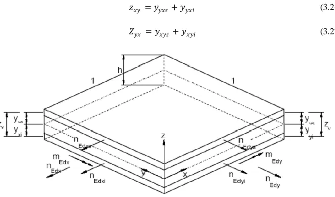
Figure 3-2 Generic shell element forces per unit width (adapted Flügge, 1973). ... 41

Figure 3-3 Membrane forces in translation shells (Billington, 1982). ... 42

Figure 3-4 Generic hyperbolic paraboloid... 44

Figure 3-5 Generic elliptical paraboloid. ... 45

Figure 3-6 Example of Mesh with: a) quadratic elements; b) triangular elements. ... 47

Figure 3-7 Shape functions(Azevedo, 2003). ... 48

Figure 3-8 Obtained hyperboloid paraboloid shell. ... 49

Figure 3-9 Representation of: a) FEM 1 model; b) FEM 2 model. ... 50

Figure 3-10 FEM 1's map of membrane forces in: a) x-direction; b) y-direction. Units in kN/m. 51 Figure 3-11 FEM 2's map of membrane forces in: a) x-direction; b) y-direction. Units in kN/m. 51 Figure 3-12 Representation of the "Direction A" line and "Direction B" line. ... 52

Figure 3-13 Membrane forces in the x-direction that "overlap" the Direction A line. ... 53

Figure 3-14 Membrane forces in the y-direction that "overlap" the Direction A line. ... 53

Figure 3-15 Membrane forces in the x-direction that "overlap" the Direction B line. ... 54

Figure 3-16 Membrane forces in the y-direction that "overlap" the Direction B line. ... 54

Figure 3-17 Obtained elliptical paraboloid shell. ... 55

Figure 3-18 Representation of the FEM 3 model. ... 57

Figure 3-19 FEM 3's map of membrane forces in the: a) x-direction; b) y-direction. Units in kN/m. ... 57

(17)

xiv

Figure 3-20 Membrane forces in the x-direction that "overlap" the Direction A line. ... 58

Figure 3-21 Membrane forces in the y-direction that "overlap" the Direction B line. ... 58

Figure 3-22 Membrane forces in the y-direction that "overlap" the Direction A line. ... 59

Figure 3-23 Membrane forces in the x-direction that "overlap" the Direction B line. ... 59

Figure 3-24 Sandwich model layers (Cardoso, 2008). ... 61

Figure 3-25 Axial actions and bending moments in the outer layer (EN 1992-2, 2005)... 62

Figure 3-26 Membrane shear actions and twisting moments in the outer layer (EN 1992-2, 2005). ... 63

Figure 3-27 Schematic representation of a strut and tie model. ... 66

Figure 3-28 Mohr's Circle for the biaxial compression state (compressions assumed as positive) (Cardoso, 2008)... 68

Figure 3-29 Thin plate: a) at initial configuration with only membrane forces; b) with lateral load applied; c) at displaced position due to lateral load. ... 71

Figure 3-30 Buckling versus Strength (Ramm, 1987). ... 71

Figure 3-31 Reduction of the buckling critical load according to the IASS (Ramm, 1981). ... 73

Figure 3-32 Imperfection sensitivity factor (adapted IASS, 1979). ... 74

Figure 3-33 Values of the parameter 𝜳 (adapted IASS, 1979). ... 75

Figure 3-34 Cracking and reinforcement factor (adapted IASS, 1979) ... 75

Figure 4-1 Schematic representation of the desired interoperability. ... 85

Figure 4-2 NURBS curve in: a) initial position; b) updated position. ... 86

Figure 4-3 NURBS surface in: a) initial position; b) updated position. ... 87

Figure 4-4 Grasshopper Interface. ... 88

Figure 4-5 Construct point component dragged into canvas. ... 89

Figure 4-6 Slider components and geometry preview. ... 89

Figure 4-7 Creation of a parametric NURBS curve model. ... 90

Figure 4-8 Alteration of the NURBS curve. ... 90

Figure 4-9 Creation of a parametric NURBS surface model. ... 91

Figure 4-10 Alteration of the NURBS surface. ... 91

Figure 4-11 Simulation algorithm inside grasshopper. ... 92

Figure 4-12 Falling particle simulation result. ... 93

(18)

xv

Figure 4-14 Falling particle with a spring simulation result... 94

Figure 4-15 Falling particle with several springs simulation result. ... 94

Figure 4-16 Falling particle towards a piece of cloth simulation result. ... 94

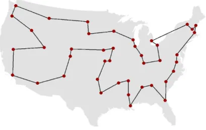
Figure 4-17 Recreation of the TSP solution obtained by George Dantzig, Ray Fulkerson and Selmer Johnson (adapted Cook, 2013). ... 95

Figure 4-18 Algorithm created to solve the TSP problem. ... 96

Figure 4-19 Overview of the created algorithm for the TSP problem... 97

Figure 4-20 Galapagos interface and results for the TSP problem. ... 97

Figure 4-21 Results obtained by: a) Dantiz, Fulkerson and Johnson; b) the genetic solver. ... 98

Figure 4-22 Importing Robot Structural Analysis dynamic-link library. ... 99

Figure 4-23 Bar created through API. ... 99

Figure 4-24 "Formfinding" custom component dragged onto the canvas. ... 100

Figure 4-25 Input of the boundary curve, defining the number of divisions, definition of anchor points and preview of the particle-spring system . ... 101

Figure 4-26 Final configuration of the created algorithm in Grasshopper and the resulting equilibrium shape in Rhinoceros 3D. ... 102

Figure 4-27 Resulting shapes from iteration: a)10; b) 100; c) 1000; d) 5000. ... 102

Figure 4-28 Equilibrium shape with: a) original stiffness; b) low stiffness. ... 103

Figure 4-29 "Robot Structural Analysis" custom plug- in... 104

Figure 4-30 Inputting a surface and Boolean toggles into the custom component. ... 105

Figure 4-31 Thickness and Mesh size inputs... 105

Figure 4-32 Surface with 4 by 4 divisions and model preview. ... 106

Figure 4-35 Components to aid the creation of beams and preview of beams in the shell. ... 107

Figure 4-36 Bar sections and reinforcement inputs. ... 108

Figure 4-37 Output results from the represented geometry. ... 109

Figure 4-38 Remote panel in Rhinoceros 3D to enable interoperability. ... 111

Figure 4-39 Example of a geometry and its analysis using the custom component. ... 112

Figure 4-40 New geometry and its analysis using the custom component. ... 112

(19)

xvi

Figure 4-42 Galapagos component connected to the desired inputs and the final result. ... 114

Figure 4-43 Results in the Galapagos interface. ... 114

Figure 4-44 Maps of vertical displacements of the: a) original structure; b) final result. Units in cm... 115

4-45 Initial geometry and points. ... 115

Figure 4-46 Map of vertical displacements of the: a) original structure; b) obtained result at the end of the morphogenetic process. Units in cm. ... 116

Figure 4-47 Map of vertical displacements of the: a) obtained result at the end of the morphogenetic process; b) catenary. Units in cm. ... 116

Figure 4-48 Teshima Art Museum in 2010 and during construction phase (Sasaki, 2014). ... 117

Figure 4-49 Wailings and struts connected (Doka Industrie, 2012). ... 118

Figure 4-50 Beams connected to wailings (Doka Industrie, 2012). ... 118

Figure 4-51 Profiled timber forms connected to beams (Doka Industrie, 2012). ... 119

Figure 4-52 Panels connected to the profiled timber forms (Doka Industrie, 2012). ... 119

Figure 4-53 Formwork component. ... 120

Figure 4-54 Formwork component inserted in Grasshopper and result presented in Rhinoceros 3D viewport. ... 121

Figure 4-55 Updated results of the formwork component. ... 122

Figure 5-1 BPMN representation of stage 1. ... 124

Figure 5-5 Shell structure based on a conoid geometry (Cardoso, 2008). ... 128

Figure 5-6 Resulting shape view from: a) Top; b) Front; c) Right. ... 129

Figure 5-7 Model created in Robot Structure Analysis with the created component. ... 130

Figure 5-8 Map of membrane forces in the x-direction for the fundamental combination with the leading variable - imposed load: a) original case; b) recreated model. Units in kN/m. ... 132

Figure 5-9 Map of membrane forces in the y-direction for the fundamental combination with the leading variable - imposed load: a) original case; b) recreated model. Units in kN/m. ... 132

Figure 5-10 Map of vertical displacements for the quasi-permanent combination: a) original case; b) recreated model. Units in cm. ... 133

(20)

xvii Figure 5-11 Particle-spring system: a) initial conditions; b) resultant shape view from the front; c)

resultant shape view from a perspective. ... 135

Figure 5-12 Proposed parametric model... 136

Figure 5-13 Results from the evolutionary solver. ... 137

Figure 5-14 Comparison between: a) the original geometry; b) the new geometry. ... 137

Figure 5-15 Structure obtained at the end of the morphogenetic process. ... 138

Figure 5-16 Map of vertical displacements for the: a) original shape; b) new shape. Units in cm. ... 138

Figure 5-17 Map of membrane forces in the x-direction for the: a) original shape; b) new shape. Units in kN/m. ... 139

Figure 5-18 Map of membrane forces in the y-direction for the: a) original shape; b) new shape. Units in kN/m. ... 140

Figure 5-19 Bending moments in the x-direction for the: a) original shape; b) new shape. Units in kN.m/m. ... 140

Figure 5-20 Bending moments in the y-direction for the: a) original shape; b) new shape. Units in kN.m/m. ... 141

Figure 5-21 Deformation due to buckling correspondent to: a) Mode 1; b) Mode 2. ... 142

Figure 5-22 Created model with beams. ... 143

Figure 5-23 Map of vertical displacements for the structure: a) without beams; b) with beams. Units in cm... 143

Figure 5-24 Map of membrane forces in the x-direction for the structure: a) without beams; b) with beams. Units in kN/m. ... 144

Figure 5-25 Map of membrane forces in the y-direction for the structure: a) without beams; b) with beams. Units in kN/m. ... 144

Figure 5-26 Map of bending moments in the x-direction for the structure: a) without beams; b) with beams. Units in kN.m/m. ... 145

Figure 5-27 Map of bending moments in the y-direction for the structure: a) without beams; b) with beams. Units in kN.m/m. ... 145

Figure 5-28 Curves and control points used in the parametric model to define the geometry. ... 147

Figure 5-29 Results presented in the Galapagos interface for the: a) first process; b) second process. ... 148

(21)

xviii

Figure 5-30 Resulting geometry of the morphogenetic process. ... 148

Figure 5-31 FEM model based on the obtained geometry at the end of morphogenetic process. 149 Figure 5-32 Map of vertical displacements for the: a) original shape; b) morphogenetic shape. Units in cm. ... 149

Figure 5-33 Map of membrane forces in the x-direction for the: a) original shape; b) morphogenetic shape. Units in kN/m. ... 150

Figure 5-34 Map of membrane forces in the y-direction for the: a) original shape; b) morphogenetic shape. Units in kN/m. ... 151

Figure 5-35 Bending moments in the x-direction for the: a) original shape; b) morphogenetic shape. Units in kN.m/m. ... 151

Figure 5-36 Bending moments in the y-direction for the: a) original shape; b) morphogenetic shape. Units in kN.m/m. ... 152

Figure 5-37 Deformation due to buckling correspondent to: a) Mode 1; b) Mode 2. ... 153

Figure 5-38 Representation of the new thickness of the shell. ... 154

Figure 5-39 Three dimensional model of the market and dimensions. Units in meters. ... 155

Figure 5-40 Additional dimensions of the market. Units in meters. ... 155

Figure 5-41 Created FEM model of the original market roof. ... 156

Figure 5-42 Formfinding process: a) initial conditions; b) resulting shape. ... 157

Figure 5-43 Parametric model of an arch in: a) initial position; b) updated position. ... 157

Figure 5-44 Arch disposition view from: a) perspective; b) top (units in meters). ... 158

Figure 5-45 FEM model of the proposed new roof. ... 158

Figure 5-46 Map of vertical displacements for the: a) original shape; b) new shape (solution 1). Units in cm. ... 159

Figure 5-47 Membrane forces in the x-direction for the: a) original shape; b) new shape (solution 1). Units in kN/m. ... 160

Figure 5-48 Membrane forces in the y-direction for the: a) original shape; b) new shape (solution 1). Units in kN/n. ... 160

Figure 5-49 Solar vectors for the day 9 of January from 6am to 7pm and: a) original configuration of supports; b) new configuration of supports. ... 162

(22)

xix Figure 5-51 Schematic representation of the 11 catenary curves in the parametric model that define the surface. ... 163 Figure 5-52 Solar vectors for the day 1 of August. ... 164 Figure 5-53 Solution of the morphogenetic process. ... 164 Figure 5-54 Solar exposition at: a) winter time in the morning; b) summer time in the morning; c) winter time in the afternoon; d) winter time in the afternoon. ... 165 Figure 5-55 FEM model representing the shape obtained through the morphogenetic process. 166 Figure 5-56 Map of vertical displacements for solution 2. Units in cm. ... 166 Figure 5-57 Map of membrane forces in the x-direction for solution 2. Units in kN/m. ... 167 Figure 5-58 Map of membrane forces in the y-direction for solution 2. Units in kN/m. ... 167 Figure I-1 Map of vertical Displacement for the: a) Arch 1 (catenary); b) Arch 2; c) Arch 3. Units in cm. ... 183 Figure I-2 Map of membrane forces in the x-direction for the: a) Arch 1 (catenary); b) Arch 2; c) Arch 3. Units in kN/m. ... 183 Figure I-3 Map of membrane forces in the y-direction for the: a) Arch 1 (catenary); b) Arch 2; c) Arch 3. Units in kN/m. ... 183 Figure I-4 Map of shear forces in the xy-direction for the: a) Arch 1 (catenary); b) Arch 2; c) Arch 3. Units in kN/m. ... 184 Figure I-5 Map of shear forces in the x-direction for the: a) Arch 1 (catenary); b) Arch 2; c) Arch 3. Units in kN/m. ... 184 Figure I-6 Map of shear forces in the y-direction for the: a) Arch 1 (catenary); b) Arch 2; c) Arch 3. Units in kN/m. ... 184 Figure I-7 Map of bending moments in the x-direction for the: a) Arch 1 (catenary); b) Arch 2; c) Arch 3. Units in kN.m/m. ... 185 Figure I-8 Map of bending moments in the y-direction for the: a) Arch 1 (catenary); b) Arch 2; c) Arch 3. Units in kN.m/m. ... 185 Figure I-9 Map of twisting moments in the xy-direction for the: a) Arch 1 (catenary); b) Arch 2; c) Arch 3. Units in kN.m/m. ... 185 Figure I-10 Map of principal stresses S1 of the: a) Arch 1 (catenary); b) Arch 2; c) Arch 3. Units in MPa... 186

(23)

xx

Figure I-11 Map of principal stresses S2 of the: a) Arch 1 (catenary); b) Arch 2; c) Arch 3. Units in MPa. ... 186 Figure II-1 -Map of vertical displacements of: a) spherical dome; b) catenary shaped dome. Units in cm... 188 Figure II-2 Map of membrane forces in the hoop direction of: a) spherical dome; b) catenary shaped dome. Units in kN/m... 188 Figure II-3 Map of membrane forces in the meridional direction of: a) spherical dome; b) catenary shaped dome. Units in kN/m. ... 188 Figure II-4 Map of bending forces in the hoop direction of: a) spherical dome; b) catenary shaped dome. Units in kN.m/m... 189 Figure II-5 Map of bending forces in the meridional direction of: a) spherical dome; b) catenary shaped dome. Units in kN.m/m... 189 Figure II-6 Map of shear forces in the hoop direction of: a) spherical dome; b) catenary shaped dome. Units in kN/m. ... 189 Figure II-7 Map of shear forces in the meridional direction of: a) spherical dome; b) catenary shaped dome. Units in kN/m... 190 Figure II-8 Map of principal stresses S1 of: a) spherical dome; b) catenary shaped dome. Units in MPa. ... 190 Figure II-9 Map of principal stresses S2 of: a) spherical dome; b) catenary shaped dome. Units in MPa. ... 190 Figure III-1 Map of membrane forces in the x-direction for the structure obtained by the: a) network of chains; b) piece of cloth. Units in kN/m. ... 191 Figure III-2 Map of membrane forces in the y-direction for the structure obtained by the: a) network of chains; b) piece of cloth. Units in kN/m. ... 191 Figure III-3 Map of shear forces in the-xy direction for the structure obtained by the: a) network of chains; b) piece of cloth. Units in kN/m. ... 192 Figure III-4 Map of bending moments in the x-direction for the structure obtained by the: a) network of chains; b) piece of cloth. Units in kN.m/m... 192 Figure III-5 Map of bending moments in the y-direction for the structure obtained by the: a) network of chains; b) piece of cloth. Units in kN.m/m... 193

(24)

xxi Figure III-6 Map of twisting moments in the xy-direction for the structure obtained by the: a) network of chains; b) piece of cloth. Units in kN.m/m. ... 193 Figure III-7 Map of principal stresses S1 for the structure obtained by the: a) network of chains; b) piece of cloth. Units in MPa. ... 194 Figure III-8 Map of principal stresses S2 for the structure obtained by the: a) network of chains; b) piece of cloth. Units in MPa. ... 194 Figure V-1Cross representations of the principal stresses in the FEM 2 model ... 198 Figure V-2 Map of vertical Displacement for the: a) FEM 1 model; b) FEM 2 model. Units in cm. ... 199 Figure V-3 Map of membrane forces in the x- direction for the: a) FEM 1 model; b) FEM 2 model. Units in kN/m. ... 199 Figure V-4 Map of membrane forces in the y-direction for the: a) FEM 1 model; b) FEM 2 model. Units in kN/m. ... 200 Figure V-5 Map of shear forces in the xy-direction for the: a) FEM 1 model; b) FEM 2 model. Units in kN/m. ... 200 Figure V-6 Map of bending moments in the x-direction for the: a) FEM 1 model; b) FEM 2 model. Units in kN.m/m. ... 201 Figure V-7 Map of bending moments in the y-direction for the: a) FEM 1 model; b) FEM 2 model. Units in kN/m. ... 201 Figure V-8 Map of twisting moments in the xy direction for the: a) FEM 1 model; b) FEM 2 model. Units in kN.m/m. ... 202 Figure VI-1 Cross representation of the stresses ... 203 Figure VI-2 Map of vertical Displacement for the FEM 3 model. Units in cm. ... 204 Figure VI-3 Map of membrane forces in the x-direction for the FEM 3 model. Units in kN/m. 204 Figure VI-4 Map of membrane forces in the y-direction for the FEM 3 model. Units in kN/m. 205 Figure VI-5 Map of shear forces in the xy-direction for the FEM 3 model. Units in kN/m. ... 205 Figure VI-6 Map of bending moments in the x-direction for the FEM 3 model. Units in kN.m/m. ... 206 Figure VI-7 Map of bending moments in the y-direction for the FEM 3 model. Units in kN.m/m. ... 206

(25)

xxii

Figure VI-8 Map of twisting moments in the xy-direction for the FEM 3 model. Units in kN.m/m. ... 207 Figure VII-1 Open new project ... 208 Figure VII-2 Create new material ... 208 Figure VII-3 Create two nodes and a bar ... 208 Figure VII-4 Create a section and apply to the bar with the created material ... 209 Figure VII-5 Create supports and calculate ... 209 Figure VIII-1 Original geometry proposed in (Cardoso, 2008)... 210 Figure VIII-2 New geometry obtained in solution 1 ... 211 Figure VIII-3 Comparison between the original curve 1 and the new ... 212 Figure VIII-4 Comparison between the original curve 2 and the new ... 212 Figure VIII-5 Comparison between the original curve 3 and the new ... 212 Figure IX-1 Map of shear forces in the xy-direction for the: a) original shape; b) new shape. Units in kN/m. ... 213 Figure IX-2 Map of twisting moments in the xy-direction for the: a) original shape; b) new shape. Units in kN.m/m... 213 Figure IX-3 Map of principal stresses S1 for the: a) original shape; b) new shape. Units in MPa. ... 214 Figure IX-4 Map of principal stresses S2 for the: a) original shape; b) new shape. Units in MPa. ... 214 Figure X-1 Map of shear forces in the xy-direction: a) new without beams; b) new with beams. Units in kN/m... 215 Figure X-2 Map of twisting moments in the xy-direction: a) new without beams; b) new with beams. Units in kN.m/m. ... 215 Figure X-3 Map of principal stresses S1: a) new without beams; b) new with beams. Units in MPa. ... 216 Figure X-4 Map of principal stresses S2: a) new without beams; b) new with beams. Units in MPa. ... 216 Figure XI-1 Original geometry proposed in (Cardoso, 2008) ... 217 Figure XI-2 Obtained geometry at the end of the morphogenetic process ... 218

(26)

xxiii Figure XI-3 Comparison between the original curve 1 and the obtained at the of the morphogenetic process ... 219 Figure XI-4 Comparison between the original curve 2 and the obtained at the of the morphogenetic process ... 219 Figure XI-5 Comparison between the original curve 1 and the obtained at the of the morphogenetic process ... 219 Figure XII-1 Map of shear forces in the xy-direction: a) original shape; b) morphogenetic shape. Units in kN/m. ... 220 Figure XII-2 Map twisting moments in the xy-direction: a) original shape; b) morphogenetic shape. Units in kN.m/m. ... 220 Figure XII-3 Map of principal stresses stress S1: a) original shape; b) morphogenetic shape. Units in MPa... 221 Figure XII-4 Map of principal stresses S2: a) original shape; b) morphogenetic shape. Units in MPa. ... 221 Figure XIII-1 Geometry proposed in solution 1. ... 223 Figure XIII-2 Comparison between the original roof and the geometry proposed in solution 1. 223 Figure XIV-1 Map of shear forces in the xy-direction for the: a) original shape; b) new shape (solution 1). Units in cm. ... 224 Figure XIV-2 Map of bending moments in the x-direction for the: a) original shape; b) new shape (solution 1). Units in kN.m/m. ... 225 Figure XIV-3 Map of bending moments in the y-direction for the: a) original shape; b) new shape (solution 1). Units in kN.m/m. ... 225 Figure XIV-4 Map of twisting moments in the xy-direction for the: a) original shape; b) new shape (solution 1). Units in kN.m/m... 226 Figure XIV-5 Map of principal stresses S1 for the: a) original shape; b) new shape (solution 1).. Units in MPa. ... 226 Figure XIV-6 Map of principal stresses S2 for the: a) original shape; b) new shape (solution 1). Units in MPa. ... 227 Figure XV-1 Shape resulting of: a) formfinding process; b) morphogenetic process. ... 228 Figure XV-2 Comparison between the geometry obtained at the end of the formfinding process and the solution obtained using the morphogenetic process. ... 229

(27)

xxiv

Figure XVI-1 Map of shear forces in the xy-direction for solution 2. Units in kN/m. ... 230 Figure XVI-2 Map of bending moments in the x-direction for solution 2.. Units in kN.m/m. ... 230 Figure XVI-3 Map of bending moments in the y-direction for solution 2. Units in kN.m/m. .... 231 Figure XVI-4 Map of twisting moments in the xy-direction for solution 2. Units in kN.m/m. .. 231 Figure XVI-5 Map of principal stresses S1 for solution 2. Units in MPa. ... 232 Figure XVI-6 Map of principal stresses S2 for solution 2. Units in MPa. ... 232

(28)

xxv

INDEX OF TABLES

Table 3-1 Acting forces on the elliptical paraboloid shell. ... 56 Table 3-2 Safety factor for a generic shell with a thickness of 15 cm using C20/25 concrete. ... 78 Table 3-3 Safety factor for a generic shell with a thickness of 15 cm using C30/37 concrete. ... 78 Table 5-1 Minimum reinforcemenet needed as determined in (Cardoso, 2008). ... 133 Table 5-2 Minimum reinforcement determined by the custom component. ... 134 Table 5-3 Minimum reinforcement needed for the new shape determined by the created component... 141 Table 5-4 Safety factors for the original and new shape. ... 142 Table 5-5 Minimum reinforcement determined by the custom component for the structure with beams. ... 146 Table 5-6 Safety factors for all the studied structures. ... 146 Table 5-7 Minimum reinforcement determined by the custom component for the structure obtained at the end of the morphogenetic process. ... 152 Table 5-8 Safety factors of the structure obtained at the end of the morphogenetic process. ... 153 Table 5-9 Safety factors of the structure with increased thickness. ... 154 Table 5-10 Reinforcement calculated by the custom component for solution 1. ... 161 Table 5-11 Safety factors of the proposed new shape (solution 1). ... 161 Table 5-12 Reinforcement calculated by the custom component for solution 2. ... 168 Table 5-13 Safety factors of the proposed new shape (solution 2). ... 168 Table I-1 Details about the geometries of Arch 1(catenary), Arch 2 and Arch 3 ... 182 Table II-1 Details about the domes' geometry ... 187 Table IV-1 Coefficients for 𝒄𝟏𝒄𝟐 = 𝟏, 𝟎 ... 195 Table IV-2 Coefficients for 𝒄𝟏𝒄𝟐 = 𝟎, 𝟖 ... 195 Table IV-3 Coefficients for 𝒄𝟏𝒄𝟐 = 𝟎, 𝟖 ... 196 Table IV-4 Coefficients for 𝒄𝟏𝒄𝟐 = 𝟎, 𝟔 ... 196 Table IV-5 Coefficients for 𝒄𝟏𝒄𝟐 = 𝟎, 𝟐 ... 197 Table VIII-1 Details about the initial geometry proposed in (Cardoso, 2008)... 210 Table VIII-2 Details about the new Geometry obtained in solution 1 ... 211

(29)

xxvi

Table XI-1 Details about the original geometry proposed in (Cardoso, 2008) ... 217 Table XI-2 Details about the geometry obtained at the of the morphogenetic process ... 218 Table XIII-1 Details about the geometry proposed (Solution 1) ... 222 Table XV-1 Details about the shape obtained by the formfinding and morphogenetic process. 228 Table XV-2 Details about the shape obtained by the formfinding and morphogenetic process (cont.) ... 229

(30)

1

1. INTRODUCTION

1.1. Scope and motivation

Recently, the modern advances in computational applications for architectural modeling have stimulated the imagination of Architects, which in turn are creating rather complex and abstract geometries usually referred to as freeform (Vizotto, 2010). Associated with this, comes a re-awakening of interest in thin shell structures since they provide freedom of design and are able to create eye-catching forms (Ochsendorf & Block, 2014). A thin shell can be defined as a surface element described by a three-dimensional curved surface, in which one dimension (the thickness) is significantly smaller than the other two. As an example of this type of structures, the National Museum Honestino Guimarães in Brasilia/Brazil is presented in Figure 1-1a). The Tenerife Concert Hall in Tenerife/Spain is also an interesting example, as shown Figure 1-1b).

Figure 1-1 a) National Museum Honestino Guimarães in Brasilia (Inojosa, 2010); b) Tenerife Conce rt Hall in Tenerife (Lightgruppe Gantenbrink, 2005).

Thin shells are highly dependent on their shape to obtain proper structural performance (Tomás & Martí, 2010), and when a proper shape is defined they are able to overcome large spans efficiently and economically without compromising the aesthetic component. Two remarkable

(31)

2

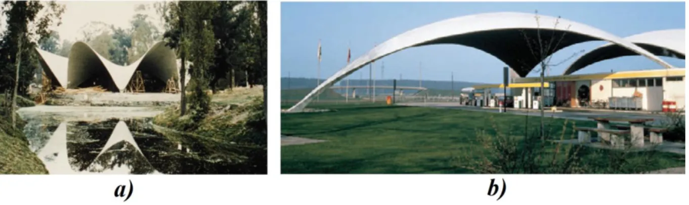
examples of such efficiency and aesthetics can be found in the wo rks by Félix Candela (see Figure 1-2a) and Heinz Isler (see Figure 1-2b). Their works become more relevant when one considers the fact that they were made in the beginning of the second half of the twentieth century without the aid of advanced analysis tools, using only simplified calculation methodologies to study the structural behavior and physical models to define the geometry (Billington, 1982).

Figure 1-2 a) Restaurant Los Manantiales in Xochimilco; b) BP Service Station in Deitingen (Garlock & Billington, 2014).

These iconic structures were only created because the structural artists that idealized them possessed three important characteristics as stated by Garlock and Billington (2014): "the ethos of

efficiency, the ethic of economy and the aesthetic motivation in design". In this context, efficiency

consists in obtaining a structure that minimizes the use of materials with sound performance and assured safety, whereas economy is related to the minimization of construction costs consistent with low expenses for maintenance.

Nowadays, however, very rarely these traits are associated with a s ingle entity, dividing the characteristics into separate roles: the Architect and the Engineer (Schlaich, 2014). Allied with this division is the frequent lack of dialog between both parts, which in turn translates into an absence of synergy between structural and architectural aspects due to improper structure shape definitions by the Architect. While in other related engineer ing disciplines (such as aerospace or automobile) or much older trades (such as ship building or armory), optimization and modification of the geometries is commonplace, this does not generally occur in the creation of structures due to time and cost constraints (Ney & Adriaenssens, 2014). This means that the

(32)

3 dialogue between the Architects and the Engineer in early stages of development is a very important process.

In situations where this important dialog occurs, the interactive processes between the Architect and the Engineer to define the shape, even with the modern advances in computational applications, is still relatively slow, with a large time gap between the conceptual discussion of the structure geometry and the definition of solutions for discussions. In fact, the analysis of a thin reinforced concrete shell requires the creation of rather complex three-dimensional models, which sometimes can be time consuming and difficult (Borgart & Eigenraam, 2012).

However, the possibility of developing automatic co nnections between software applications, commonly referred as interoperability, has become increasingly accessible (Microsoft Corporation, 2014). This allows the possibility of developing specific applications to assist the interaction between Architects and Engineers in the creation of thin shell structures since early stages of the design.

1.2. Objectives

The aim of this work is to address the challenges and opportunities that are posed to the structural design of thin concrete shells by: (i) the availability of software applications capable of modeling arbitrary geometries, and (ii) their automatic interoperability with structural analysis software. It is remarked that such interoperability is achieved through a custom-devised application, and supported by the use of generative algorithms and shape optimization strategies.

In a more specific way, the achievement of the main goal highlighted above is pursued by a set of partial objectives throughout this work which comprise, first of all, a critical discussion of the historical background and advantages of structures based on thin reinforced concrete shells, highlighting the features that make them so special. Based on the obtained information, it is intended to understand and implement some of the existing design techniques, namely the use of physical models to define and optimize the shape of a structure by a technique known as formfinding. Furthermore, it is intended to deepen the study of a modern trend known as

(33)

4

morphogenesis, which is based on the use of the genetic algorithms, as an additional optimization technique for the shape definition of thin shell structures.

In order to aggregate all the obtained knowledge, a set of user-friendly software applications will be created to assist the design of thin reinforced concrete shells. The most important of such applications is centered in enabling real- time interoperability between a modeling software based on the NURBS1 technology and a structural analysis software based on the finite element method. This application will allow the user to define a geometry of a possible structure directly in the modeling software, and any changes that are performed to the geometry of the structure are automatically updated in the structural analysis software, thus allowing an interactive structural analysis. In addition, it is intended that the tool will be able to compute stresses/strains of the structure, returning the corresponding information in real- time. The developed application also incorporates evaluation of results issued by the structural analysis software, with automatic verifications of limit states, and even the calculation of the necessary reinforcement for the shell. In the same application, it is intended to integrate genetic algorithms in order to perform an automatic processes of shape optimization.

Lastly, and taking into account all the concepts learned during the course of this dissertation in junction with the developed applications, it is intended to propose a framewo rk of interaction between an Architect and an Engineer for early pre-design stages of a thin shell structure, capable of obtaining an optimized structure. The created framework will be the implemented in a set of hypothetical scenarios in order to try to obtain thin reinforced concrete shell structures capable of performing the design requirements efficiently.

The aim of the set of proposed interfaces and methodologies is to promote and encourage the interaction between the Architect and the Engineer, especially during early stages of development in the context of thin concrete shell whose performance is especially influenced by geometric conditions. Effective dialogue and high interoperability between software applications will hopefully provide the necessary conditions to perform the design of aesthetically pleasing structures using optimized quantities of materials and controlled execution costs.

(34)

5

2. FORMFINDING AND MORPHOGENESIS OF THIN CONCRETE

SHELLS

2.1. General remarks

The ideal goal of all structural designers was summarized by A.M. Haas, who wrote (1971, apud Bellés, et. al, 2009) "To obtain the greatest structural efficiency, the designer must select a shape

which, under the project conditions, approximates to membrane stress state as much as possible and in consequence, reduces bending or secondary stresses to a minimum. This is not only simple from the analysis viewpoint, but also provides the lowest cost structural solution ". Although Hass

was referring to structures in general, his statement has even more relevance when referring to thin shell elements since they have greater in-plane stiffness when in comparison with bending stiffness, due to the reduced thickness when compared with the other two dimensions. If the proposed goal by Haas is achieved, and the entire structure is mainly under membrane stress, the entire shell section would have stress uniformly applied thus allowing the full employment of the material's bearing capacity (Ramm & Melhorn, 1991). In the case of thin shells made of concrete, the material's higher compressive resistance in relation to tensile resistance should be taken into account; therefore the structure should be designed to favor this aspect (Tomás & Martí, 2010). In order to achieve the goal desired by Hass, the design of a structure cannot be done by traditional methods. Traditionally when designing structures, the geometry determines the behavior of the structure, while in this case the opposite must be achieved, meaning the behavior determines the shape. The process of defining geometry according to the intended behavior defines the term formfinding (Tysmans, 2013).

This chapter presents a brief historical insight into formfinding and its creators, as well as several classical and modern techniques for achieving optimum geometry through formfinding. In addition, some examples of the importance of a shape in a shell will be given. Ultimately, a trending technique in finding shapes, known as morphogenesis, will be presented.

(35)

6

2.2. History of thin shells and physical formfinding

One of the earliest examples of formfinding is attributed to Robert Hooke, most known for Hooke's law of elasticity. In 1675, the English scientist discovered "the true mathematical and

mechanical form of all manner of arches for building", which he then summarized in the

following statement: "As hangs the flexible line, so but inverted will stand the rigid arch " (Block, DeJong, & Ochsendorf, 2006). This relation between a flexible line and an arch can be explained with the example of a hanging chain as shown in Figure 2-1. If a chain with constant weight per unit length is hung by its two extremities (points B and C), it will eventually reach an equilibrium state under pure stress since it has no bending stiffness. If the equilibrium shape is inverted to the shape of an arch, the equilibrium state corresponds to pure compression.

Figure 2-1 Poleni’s drawing of Hooke’s analogy between an arch and a hanging chain (Block, DeJong, & Ochsendorf, 2006).

The obtained equilibrium shape is referred to as a catenary (from the Latin word "catena" meaning chain) which represents the shape of a hanging chain when only subject to gravitational force. This shape can be derived mathematically and is represented by the following equation:

𝑦 = 𝑎 × 𝑐𝑜𝑠𝑕 𝑥

(36)

7 where y represents the y-coordinate, x the x-coordinate and a is a parameter that changes the length of the chain as presented in Figure 2-2.

Figure 2-2 Representation of three catenary curves.

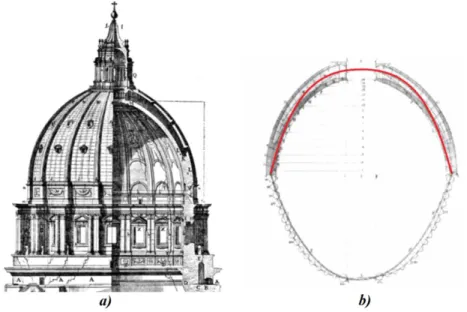
In 1748, Giovanni Poleni analyzed a real structure using Hooke's idea to assess the safety of St. Peter's dome in Rome (schematically presented in Figure 2-3a). Using the principle of the hanging chain he divided the dome in slices and hung the same number of slices with weights proportional to the weights of the corresponding section. Afterwards he proved that the chain could be contained by the dome therefore the structure was considered safe as can be seen in Figure 2-3b) (Block, DeJong, & Ochsendorf, 2006).

Figure 2-3 a) Schematic representation of St. Peter's Dome; b) Poleni's analysis of St-Peter's Dome (Block, DeJong, & Ochsendorf, 2006)

0 1 2 3 4 5 6 -4 -2 0 2 4 y-coo rdi na te ( m ) x-coordinate (m) a=0.5 a=1 a=2

(37)

8

Equilibrium in an arch can be visualized using the line of thrust, which is a theoretical line that represents the path of the resultant of the compressive forces. If the line of thrust is entirely within the section, the structure is in equilibrium. This line is the inverted catenary previously discussed. For a more in-depth explanation one should refer to (Block, DeJong, & Ochsendorf, 2006).

To illustrate this idea, the following example is forwarded: Three concrete arches (density equal to 25 kN/m³), all with a span of 20 meters, a 5 meter width, 15cm thickness, and a maximum height in the middle of 4,5 meters were created. The first has the shape of a catenary, whereas the second is slightly higher between the extremities and the middle, and the third is slightly lower between the extremities and the middle. The geometrical representations of the arches are presented in Figure 2-4 as well as the equations used to create the geometries.

Figure 2-4 Three arches' geometry.

Knowing the arches' geometry, three individual structural finite element models were created to observe their performance. The displacements and bending moments of the three arches were calculated (see more details about the modeling of these examples in Appendix I), and the corresponding results are presented in Figure 2-5 and Figure 2-6.

Even though the geometry of these three arches may appear similar, the structural performance is significantly different. It is clear that the arch created with the catenary has inferior displacements

(38)

9 and bending moments when in comparison with the other arches, as evidence in Figure 2-5a) and Figure 2-6a). As expected, the catenary curve defines the line of thrust and when the other arches' geometry deviates from this theoretical line, bending moments arise which leads to an increase in displacement.

Figure 2-5 Map of vertical displacements for: a) Arch 1 (catenary); b) Arch 2; c) Arch 3. Units in cm.

Figure 2-6 Map of bending moments for: a) Arch 1 (catenary); b) Arch 2; c) Arch 3. Units in kN/m.

It is fair to state that the hanging chain principle revolutionized the way engineers designed structural arches since the late eighteenth century and many designers have experimented with hanging chain models since then. During the second half of the nineteenth century, a number of books recommended the use of hanging chain models to establish the best geometry for arches and vaults, specifically three-dimensional hanging models (Addis, 2014).

One of the most famous architects who used these methods was Antoni Gaudí, who used three-dimensional hanging models made of strings and bags of sand to help establish the shape of his buildings, and to compliment the use of statical calculations and graphical statical methods (Addis, 2014). As an example of a building created by him with the aid of this method, in Figure

(39)

10

2-7 the crypt of the unfinished Colò nia Güell is presented (Huerta, 2006) and in Figure 2-8 the respective hanging models used to define its shape. As an additional note, even though this method is often attributed to the creation of the La Sagrada Familia, some authors consider this hypothesis unlikely as demonstrated by Huerta (2006) and Tomlow (2002).

Figure 2-7 a) Original design for the Colònia Güell (Hensbergen, 2001); b) Colònia Güell's Crypt in 2008 (Canaan, 2008)

Figure 2-8 Hanging model used to define the shape of Colònia Güell: a) uncompleted and created by Gaudi (Huerta, 2006); b) recreated by othe r artist (Addis, 2014).

In the first half of the twentieth century, contrary to earlier centuries, roof shells tended to be mainly based on pure geometrical shapes. These are shapes defined by elementary analytical

(40)

11 formulae such as spheres, cylinders, elliptic, parabolo ids and hyperboloic paraboloids (Bletzinger & Ramm, 2014). One reason, of course, was that geometrical shapes could be handled by analytical shell analysis. This reflects interactions of the usual design practice and classical shell theory, which only gives closed solutions for analytically defined geometries (Bletzinger & Ramm, 1993). These classical shapes do not usually lead to a proper membrane oriented response. Consequently, extra elements such as edge beams, stiffeners and pre-stressing had to be introduced, as seen in the case of the Sydney Opera House in Sydney (Ochsendorf & Block, 2014) (seen in Figure 2-9a), and the Kresge Auditorium in Cambridge (Bletzinger & Ramm, 2014) (seen in Figure 2-9b).

Figure 2-9 a) Sydney Opera House (Utzon, 2002); b) Kresge Auditorium (Bletzinger & Ramm, 2014).

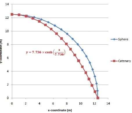
To prove the lack of membrane oriented response in the classical shapes mentioned above, the following example is presented: two individual dome geometries were calculated through the finite element method, comprising of only shell elements and pinned supports on their boundaries. The first dome is a half- sphere with a 12,5 meter radius, and the second, a surface of revolution created with a catenary similar to the sphere (see representation and mathematical formulation in Figure 2-10). Both domes are made out of concrete (self-weight of 25kN/m³), with 15cm constant thickness and solely subjected to their self- weight. Further details about these simulations can be found in Appendix II.

(41)

12

Figure 2-10 Cross-sectional representation of the two domes: sphere -based and catenary-based.

A comparison between the maps of displacements and membrane forces of both domes can be seen in Figure 2-11, Figure 2-12 and Figure 2-13. It becomes clear that the zones where the spherical dome deviates from the catenary shape correspond to the zones where tensile membrane forces arise and where the displacements are higher. Nonetheless, both shapes have negligible bending moments and consequently, low out-of-plane shearing forces (as seen in Appendix II).

Figure 2-11 - Map of ve rtical displacements: a) spherical dome; b) catenary s haped dome . Units in cm.

(42)

13

Figure 2-12 Map of me mbrane forces in the hoop direction: a) spherical dome; b) catenary shaped dome. Units in kN/m.

Figure 2-13 Map of me mbrane forces in the meridional direction: a) spherical dome; b) catenary shaped dome. Units in kN/m.

However, not all pure geometrical shapes are unusable as demonstrated by Felix Candela (Billington, 1982). Candela is known as one of the best thin shell builders (Garlock & Billington, 2014), most famous for the use of pure shapes, especially the hyperboloid paraboloids (hypar) because he knew how to best use the geometry's advantages and overcome their disadvantages. Hypar consists in translating a parabolic curve over another parabolic curve (Billington, 1982), and thus, straight lines can be generated as seen in Figure 2-14. This property of the hypar enables the use of straight formwork in the construction of the shell, therefore eliminating extra expense from customized and/or curving formwork (Draper, Garlock, & Billington, 2008). An example of this type of formwork is visible in Figure 2-15 during the construction of Chapel Lomas de Cuernavaca design by Félix Candela.

(43)

14

Figure 2-14 Hyperboloid Paraboloid with: a) curved boundaries, b) straight boundaries (Holze r, Garlock, & Prevost, 2008).

Figure 2-15 Formwork used for the creation of the Chapel (Holze r, Garlock, & Prevost, 2008).

Candela also acknowledged that one important advantage of the hypar was its double-curvature. This grants an arch-effect in two planes and, in contrast to the arch contained in only one plane, provides more ways for the internal forces to flow. Additionally, without the aid of computers and by using only simplified analytical methods, he understood where these forces would be greatest and as a result increased the thickness in these locations, for instance the edges and the supports (Billington, 1982). Even though some of Candela’s designs could be further optimized (Holzer, Garlock, & Prevost, 2008) his final results were aesthetically pleasing (see Figure 2-16) and functional without being too expensive when compared to other structural solutions.

(44)

15

Figure 2-16 Félix Candela's Chapel Lomas de Cuernavaca (Holze r, Garlock, & Prevost, 2008).

It is also important to provide a historical remark to Heinz Isler, who is commonly considered the last of the great concrete shell builders of the twentieth century, and, like many before him brought about his own unique approach (Garlock & Billington, 2014). His simple idea was to take Hooke's two-dimensional technique into the third dimension. This was possible by using a sheet of cloth (instead of a chain) to make hanging models which he then scaled up to reproduce their funicular geometry at full size as represented in Figure 2-17.

(45)

16

A technique he developed was to suspend a piece of wet cloth outdoors during a Swiss winter night, and in the morning the cloth would be frozen and static in a shape which only had membrane stresses (Addis, 2014). It is also important to notice that in this type of structures, the self-weight is most of the times, the dominant load and thus the techniques to determine the shape tended to solely consider this load acting on the structures (Chilton, 2000). In his experiments with cloths, Isler also discovered the importance of fiber orientation. Using the same textile, but simply modifying the angle of anisotropy, different shapes were obtained, as s hown respectively in Figure 2-18 where the fibers are parallel to the edges and Figure 2-19 where the fibers are diagonal to the edges.

Figure 2-18 Fibers parallel to the edge and corresponding shape (adapted Bletzinger & Ramm, 2014).

Figure 2-19 Fibers diagonal to the edge and corresponding shape (adapted Bletzinger & Ramm, 2014).

These techniques proposed by Isler generate the form of the shell, as well as the fold that provides stiffening to the free edges of the shells, as shown in the model presented in Figure 2-20b). Isler also used techniques like air pressure to inflate elastic membranes, creating surfaces with membrane forces only as seen in Figure 2-21.

(46)

17

Figure 2-20 Shell geometry: a) without the folded edge; b) with the folded edge (Tysmans, 2013).

Figure 2-21 a) Membrane unde r pressure (Chilton, 2000); b) full scale structure (Garlock & Billington, 2014).

The physical formfinding process described until now provides interesting design opportunities and stimulates creativity. In a short period of time it is possible to evaluate the influence and the importance of the boundary conditions of a structure, as well as evaluating alternative scenarios. The visual feedback of the models provides a notion of load bearing, buckling behavior and weak points in design. On the other hand, it also needs to be acknowledged that the application of physical formfinding methods has significant costs on material and time, whereas contemporary numerical tools make it possible to simulate these experiments in virtual environments. Nevertheless, there is a place for physical modeling today, as Frei Otto proved when designing the new train station in Stuttgart, Germany (2007-2013). Otto and his colleagues used innovative techniques such as hanging soap film (see Figure 2-22) and the traditional hanging chains for creating physical models for static and dynamic load analysis (see Figure 2-23) (Tysmans, 2013).

(47)

18

Figure 2-22 Soap Film used by Frei Otto (adapted Addis, 2014).

Figure 2-23 Physical model for static and dynamic load analysis (Tysmans, 2013).

2.3. Numerical formfinding

Numerical formfinding allows the simulation of the process of physical formfinding within virtual environments. These methods have all the advantages of physical formfinding in addition to the fact that they are faster, inexpensive and allow true scale modeling. The versatility of a numerical method is an added value when the need to change the geometry or boundary conditions arises for whatever reason (aesthetical, cost, etc.). Several methods can be used to perform numerical formfinding, each with its own advantages and disadvantages. This sub-section deals with a critical review on the three main methods in use nowadays: Dynamic Relaxation method, Force Density method, and Particle-Spring System method.

(48)

19

2.3.1. Dynamic relaxation method

The Dynamic Relaxation method (DRM) was proposed by Day in 1965 as an alternative analysis tool for indeterminate structures (Bagrianski & Halpern, 2013). One of the most famous applications of Dynamic Relaxation was in the definition of the shape of the glass shell roof of the Dutch Maritime Museum in Amsterdam (see Figure 2-24), by Ney and Partners in 2011 (Adriaenssens, et. al, 2012). Using equations derived from Newton's second law of motion, Dynamic Relaxation transforms a nonlinear static problem into a pseudo-dynamic one, in which the geometry is updated via a time-stepping procedure to achieve a sufficiently equilibrated state (Bagrianski & Halpern, 2013). To better understand this method, its basing formulation is presented next.

Figure 2-24 Dutch Maritime Museum in Amsterdam (Adriaenssens, et. al, 2012).

The formulation starts with Newton's second law of motion which can be expressed as the following general equation,

𝐹𝑜𝑟𝑐𝑒 = 𝑀𝑎𝑠𝑠 × 𝐴𝑐𝑐𝑒𝑙𝑎𝑟𝑎𝑡𝑖𝑜𝑛 + 𝑉𝑒𝑙𝑜𝑐𝑖𝑡𝑦 × 𝐷𝑎𝑚𝑝𝑖𝑛𝑔 + 𝐷𝑖𝑠𝑝𝑙𝑎𝑐𝑒𝑚𝑒𝑛𝑡 × 𝑆𝑡𝑖𝑓𝑓𝑛𝑒𝑠𝑠 (2.2) In Figure 2-25 a spring- mass damper system with a free node i, a fixed node j (both governed by Newton's second law), and a connecting member between the nodes m (governed by Hooke's law

(49)

20

of elasticity) is presented. By applying the general equation 2.2 in the system, the equilibrium of node i in the 𝑥-direction at time 𝑡, can be expressed as,

𝑃_𝑖𝑥 = 𝐾_𝑖𝑥. 𝛿_𝑖𝑥𝑡 + 𝐶_𝑖. 𝑣_𝑖𝑥𝑡 + 𝑀_𝑖. 𝑣 _𝑖𝑥𝑡 (2.3)

Figure 2-25 Spring-mass-damper system (adapted Adriaenssens, 2014).

where,

𝑃_𝑖𝑥 is the applied force at node 𝑖 in the 𝑥-direction 𝐾_𝑖𝑥 is the stiffness term at node 𝑖 in the 𝑥-direction

𝛿_𝑖𝑥𝑡 _{is the total displacement of node 𝑖 in the 𝑥-direction at time 𝑡} 𝐶_𝑖𝑥 is the viscous damping constant at node 𝑖

𝑣_𝑖𝑥𝑡 _{is the velocity node}_{𝑖 in the 𝑥-direction at time 𝑡} 𝑀_𝑖 is the lumped fictitious mass at node 𝑖

𝑣 𝑖𝑥𝑡 is the acceleration at node 𝑖 in the 𝑥-direction at time 𝑡

The presented equation 2.3 can be rewritten for any time 𝑡 as a function of all the external and internal forces acting on the node, as presented by the following equation,

(50)

21 ⇔ 𝑅_𝑖𝑥𝑡 _{= 𝐶}

𝑖. 𝑣𝑖𝑥𝑡 + 𝑀𝑖. 𝑣 𝑖𝑥𝑡 (2.5) where, 𝑅_𝑖𝑥𝑡 _{represents the residual (or resultant) of the applied loads (𝑃}

𝑖𝑥) and structural member forces (𝐾_𝑖𝑥𝛿_𝑖𝑥𝑡 _{) at node 𝑖 in the 𝑥-direction at time 𝑡.}

Furthermore, by expressing the acceleration (𝑣 _𝑖𝑥𝑡 _{) and velocity (𝑣}

𝑖𝑥𝑡 ) terms in equation 2.5 in central finite difference form for a small time step 𝛥𝑡, the residual forces acting on the node can be obtained by the following equation (Adriaenssens, 2014),

𝑅_𝑖𝑥𝑡 = 𝑀_𝑖 𝑣𝑖𝑥 𝑡 +𝛥𝑡 2 −𝑣_𝑖𝑥𝑡 −𝛥𝑡 2 𝛥𝑡 + 𝐶𝑖 𝑣_𝑖𝑥𝑡 +𝛥𝑡 2+𝑣_𝑖𝑥𝑡 −𝛥𝑡 2 𝛥𝑡 (2.6)

The previous equation can now be rearranged as a function of the velocity of the node, along with the introduction of a single viscous damping constant (C). This constant has the purpose of avoiding a continuous oscillation of the elements that compose the system, by reducing the velocity at each time step, until the movement stops and equilibrium is found. By introducing this constant, the equation 2.6 can be rearranged so that the updated velocity components at the time 𝑡 + ∆𝑡 2 are given by (Adriaenssens, et. al, 2014),

𝑣_𝑖𝑥𝑡+𝛥𝑡 2 = 𝐴. 𝑣_𝑖𝑥𝑡−𝛥𝑡 2 + 𝐵.𝛥𝑡 𝑀_𝑖 𝑅𝑖𝑥

𝑡 _(2.7)

where 𝐴 = 1 − 𝐶 2 1 + 𝐶 2 , 𝐵 = 1 − 𝐴 2 and C is a constant for the complete structure.

The time it takes to find the equilibrium depends on the viscous damping constant used. In order to achieve the most rapid convergence, the critical viscous damping value should be used, which in some case might be difficult to estimate (Adriaenssens, 2014).

As an alternative, it is possible to use the Kinetic Damping method (Adriaenssens, et. al, 2014). With this method there is no viscous damping, but instead all the nodal velocities are set to zero when a kinetic energy peak is detected. A kinetic energy peak corresponds to a local maximum of kinetic energy, which in turn corresponds to a local minimum of potential energy. The peak of energy is detected when the kinetic energy of the current iteration is inferior to the previous iteration. The value of this energy corresponds to the sum of the total energy at each node which can be determined by using the equation 𝐸_𝑘,𝑖 = 𝑀_𝑖× 𝑣_𝑖2.