Pastpresent and future worries: an fMRI study

(1)

Dezembro, 2014

Carolina Pinto Inverno da Piedade

Licenciatura em Ciências da Engenharia Biomédica

Past/present and future worries: an fMRI study

Dissertação para obtenção do Grau de Mestre em Engenharia Biomédica

Orientador: Gina Caetano, Investigadora Auxiliar, IBILI/ICNAS – UC

Co-orientadores: Miguel Castelo-Branco, Director, IBILI/ICNAS – UC

Pedro Vieira, Professor Auxiliar, FCT-UNL

Júri:

Presidente: Professora Doutora Carla Maria Quintão Pereira

Arguente: Professor Doutor Mário António Basto Forjaz Secca

(2)

Past/present and future worries: na fMRI study

(3)

(4)

(5)

I

Acknowledgements

This work was supported by Fundação para a Ciência e Tecnologia (PTDC/SAU-BEB/100147/2008, Pest-C/SAU/UI3282/2013), Portugal.

I would like to thank Professor Gina Caetano for her expert advise, dedication and encouragement throughout this project. It was a great pleasure to learn so much with your precious help.

I am also grateful to Professor Miguel Castelo-Branco, Director of ICNAS/IBLI, who created the experimental protocol and made this work possible by accepting me. I would also want to thank Professor Mário Secca for his dedication to Biomed-ical Engineering and for the captivating way he transmits his knowledge about Mag-netic Resonance Imaging.

I am thankful to Daniel Ruivo, who has developed the evaluation protocol and experimental design, for all the support, availability and patience throughout the end-less hours spent in data transference. I also want to thank Catarina Duarte for the MatLab implementation, as well as João Marques and Carlos Ferreira for technical support in MR acquisitions.

I thank Bernardo for his friendship and company throughout our adventure in Coimbra where I met so many good and unforgettable friends.

I am grateful for the amazing friends I met in FCT-UNL during this five year journey. Particularly, I thank Carolina for all the fun and honest moments and Nuno for the companionship, support and for always managing to make me laugh.

I would like to thank my sister Leonor, for her unconditional friendship and for inspiring me every day with her hard work.

(6)

(7)

III

Resumo

Na última década, o conhecimento sobre a estrutura e funções cerebrais foi alvo de um notável avanço, principalmente devido às numerosas técnicas de imagem desenvolvidas. De entre os estudos relacionados com a neuro-ciência, são cada vez mais comuns os estudos de neuropsiquiatria com recurso e imagem médica funcional.

O presente estudo tem como principal foco a identificação das áreas cere-brais recrutadas enquanto sujeitos controlo leem frases com as suas preocupa-ções pessoais acerca do passado/presente e do futuro. O principal objetivo é caracterizar, de forma rigorosa e em condições controlo, estas áreas cerebrais por forma a explorar as implicações de relembrar acontecimentos passa-dos/presentes ou pensar em preocupações relacionadas com o futuro. Com isto em mente, imagens de ressonância magnética funcional foram recolhidas de dez indivíduos saudáveis. Os dados adquiridos foram processados e tratados estatisticamente com recurso ao Modelo Linear Geral, ao Modelo de Efeitos Fixos e ao Modelo de Efeitos Aleatórios. Posteriormente, uma análise multi-voxel com uma técnica de “Seachlight Mapping” foi executada com o intuito de encontrar padrões de ativação cerebrais que permitissem a diferenciação entre as condições estudadas.

Os resultados obtidos indicaram prevalência de ativação cerebral durante a leitura de frases referentes a preocupações passadas/presentes em compara-ção com preocupações futuras e frases de conteúdo neutro. As principais áreas identificadas estão situadas no córtex frontal, bem como nas áreas parietais, occipitais e temporais posteriores. A preocupação, por si só, mostrou ativação do córtex parietal posterior e medial, lóbulo occipital esquerdo posterior, e do lóbulo temporal esquerdo. A análise multi-voxel permitiu identificar padrões de distinção entre condições situados principalmente nos lóbulos parietal, lím-bico e frontal.

(8)

(9)

V

Abstract

For the past decade, numerous imaging techniques gave rise to remarka-ble progresses in the understanding of brain’s structure and function. Amongst the wide variety of studies onto the field of neuroscience, neuropsychiatric re-searches with resource to neuroimaging have attracted increasing attention.

The present study will focus on the identification of brain areas recruited while normative subjects read sentences related to past/present or future wor-ries. Our main aim was to accurately characterize these brain areas while providing them with a time-stamp that would hopefully help us understand the implications of past/present memories and future envisioning in worrying episodes. With that purpose, functional magnetic resonance imaging data was collected from ten healthy individuals. The obtained data was processed and statistically treated using the General Linear Model and both Fixed and Ran-dom Effects Analysis for group-level results. Thereafter, a Multi-Voxel Pattern Analysis with Searchlight Mapping was performed in order to find patterns of activation that allow differentiation between conditions.

The obtained results indicate higher brain activation while reading sen-tences related to past/present worries when compared to future worry or neu-tral sentences. The main areas include frontal cortex, posterior parietal, occipital and temporal areas. Worrying, per se, was characterized by activation of the medial posterior parietal cortex, left posterior occipital lobe and left central temporal lobe. With the searchlight mapping approach we were able to further identify patterns of distinction between conditions, which were located in the parietal, limbic and frontal lobes.

(10)

(11)

VII

List of Contents

 ACKNOWLEDGEMENTS ... I  RESUMO ... III  ABSTRACT ... V  LIST OF CONTENTS ... VII  ABBREVIATIONS ... XI  LIST OF FIGURES ... XIII  LIST OF TABLES ... XV

1. STATE OF THE ART AND MOTIVATION ... 1

1.1) NEURAL CORRELATES OF PAST/PRESENT EVENTS RETRIEVAL AND FUTURE ENVISIONING ... 1

1.2) NEURAL CORRELATES OF WORRY AND RUMINATION IN HEALTHY CONTROLS ... 4

1.3) CLINICAL APPLICATIONS ... 7

1.4) MOTIVATION ... 8

1.5) FUNCTIONAL MAGNETIC RESONANCE IMAGING:AN OVERVIEW ... 8

 Basic Principles ... 9

 Blood–Oxygenated–Level Dependent Technique (BOLD) ... 9

 Hemodynamic Response Function (HRF) ...10

1.6) METHODS FOR STATISTICAL ANALYSIS OF FMRI DATA ... 10

 Single Subject Analysis ...11

 Group-Level Analysis ...14

 Multi-Voxel Pattern analysis ...16

2. METHODS ... 19

2.1)DATA ACQUISITION ... 19

 Participants ...19

 Task and Experimental Design ...20

 MRI Acquisition Parameters ...20

2.2)DATA PROCESSING ... 21

 Anatomical Data Processing ...22

(12)

VIII

 Overlaying Functional and Anatomical data... 25

2.3)SINGLE STUDY STATISTICAL ANALYSIS ... 26

 The General Linear Model (GLM) ... 26

3.4)GROUP-LEVEL STATISTICAL ANALYSIS ... 28

 Fixed Effects (FFX) Group Analysis with False Discovery Rate (FDR) ... 28

 Random Effects (RFX) Group Analysis with Cluster-Level Statistial Thresholding ... 28

3.5)MULTI-VOXEL PATTERN ANALYSIS (MVPA) ... 29

 Trial Estimation ... 30

 Searchlight Mapping ... 30

3. RESULTS ... 31

4.1)GROUP-LEVEL RESULTS ... 31

 Imaging Data from RFX Group-Level Analysis ... 32

Brain Areas Recruited for Past Condition > Neutral Condition ... 32

 RFX Talairach Coordinates Table ... 35

 FFX Talairach Coordinates Table ... 36

4.2)MULTI-VOXEL PATTERN RESULTS ... 39

 Imaging Results from MVPA Searchlight Mapping ... 39

 MVPA Talairach Coordinates Table ... 41

4. DISCUSSION ... 43

5.1)FUNCTIONAL DESCRIPTION OF THE RELEVANT RECRUITED BRAIN AREAS ... 44

 Recollection of Past negative events and imagining Neutral entities ... 44

 Envisioning Future Worrying episodes and imagining Neutral entities... 46

 Envisioning Future Worrying episodes and Recollection of Past negative events ... 47

 Worrying thoughts and Imagining Neutral entities ... 48

5.1)MULTI-VOXEL PATTERNS OF ACTIVATION ... 50

5. SUMMARY / CONCLUSIONS ... 53

6. FUTURE WORK ... 55

7. APPENDIX ... 57

APPENDIX 1:MULTIPLE COMPARISONS CORRECTION METHODS IN DETAIL ... 57

APPENDIX 2:BRAIN SEGMENTATION METHODS IN DETAIL ... 61

(13)

IX

APPENDIX 4:HEAD MOTION DETECTION AND CORRECTION ... 65

APPENDIX 5:REMOVAL OF LINEAR AND NON-LINEAR TRENDS ... 67

APPENDIX 6:TALAIRACH TRANSFORMATION OF ANATOMICAL DATA ... 69

APPENDIX 7:INTENSITY INHOMOGENEITY CORRECTION ... 71

(14)

(15)

XI

Abbreviations

 3D – Three-Dimentions

 4D – Four-Dimentions

 AC – Anterior Commissure

 AR – First Order Autoregressive

 BA – Brodmann Area

 EPI – Echo-planar Imaging

 FA – Fine-Tuning Alignment

 FDR – False Discovery Rate

 FFX – Fixed Effects Analysis

 fMRI – Functional Magnetic Resonance Imaging

 FWER – Family-wise Errors

 GAD – General Anxiety Disorder

 GLM – General Linear Model

 HRF – Hemodynamic Response Function

 IA – Initial Alignment

 IIHC – Intensity Inhomogeneity Correction

 MRI – Magnetic Resonance Imaging

 MVPA – Multi-Voxel Pattern Analysis

 N – Neutral

 OCD – Obsessive Compulsive Disorder

 PC – Posterior Commissure

 PCC – Posterior Cingulate Cortex

 PET – Positron Emission Tomography

 PM – Percent Accuracy

 rCBF – Regional Cerebral Blood Flow

(16)

XII

 ROI – Region-of-interest

 SMA – Supplementary Motor areas

 SVM – Support vector machine

 T2* - Real Transverse Relaxation Time  TE – Echo time

 TR – Repetition time

 V1 – Primary Visual Cortex

 V2 – Secondary Visual Cortex (Area 2)

(17)

XIII

List of Figures

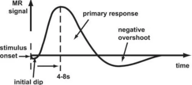
FIGURE 1.1:AN EXAMPLE OF AN HEMODYNAMIC RESPONSE FUCNTION REGARDING A SHORT STIMULUS (COLLECTED FROM KORNAK ET AL.(2011)) ... 10

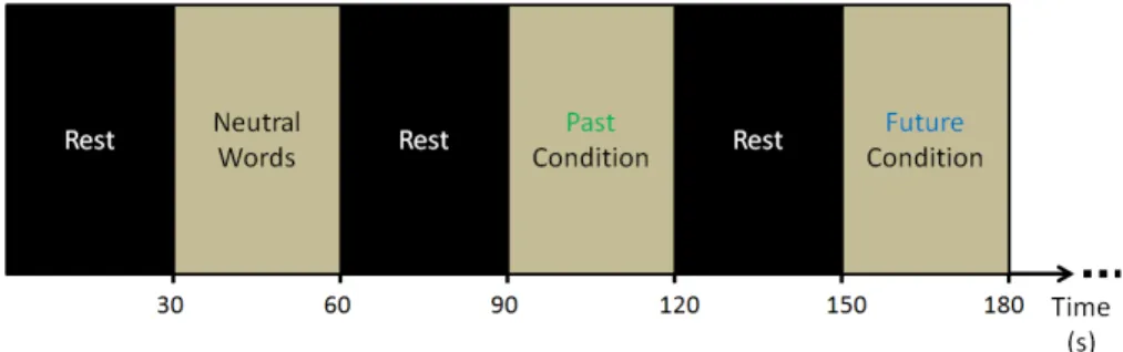
FIGURE 2.1:REPRESENTATIVE SQUEME OF THE BLOCK DESIGN PARADIGM USED IN THE PRESENT WORK.EACH BLOCK REPRESENTS THE VARIATION ACROSS TIME OF THE HEMODYNAMIC RESPONSE FUNCTION DURING ONDE SPECIFIC CONDITION. ... 20 FIGURE 2.2:DATA PROCESSING STEPS ARRANGED IN A SCHEME ... 21 FIGURE 3.1:RFXRESULTS.RELEVANT RECRUITMENT OF PRECUNEUS (BA7) FOR PAST CONDITION >NEUTRAL

CONDITION ... 32 FIGURE 3.2:RFXRESULTS.RELEVANT RECRUITMENT OF MIDDLE OCCIPITAL GYRUS (BA18) FOR PAST CONDITION

>NEUTRAL CONDITION... 32 FIGURE 3.3:RFXRESULTS.RELEVANT RECRUITMENT OF PRECENTRAL GYRUS (BA6) FOR PAST CONDITION >

NEUTRAL CONDITION ... 32 FIGURE 3.4:RFXRESULTS.RELEVANT RECRUITMENT OF MIDDLE TEMPORAL GYRUS (BA21) FOR PAST CONDITION

>NEUTRAL CONDITION... 32 FIGURE 3.5:RFX RESULTS.RELEVANT RECRUITMENT OF SUPRAMARGINAL GYRUS (BA40) FOR NEUTRAL

CONDITION >FUTURE CONDITION ... 33 FIGURE 3.6:RFX RESULTS.RELEVANT RECRUITMENT OF PRIMARY VISUAL CORTEX (BA17) FOR PAST CONDITION > FUTURE CONDITION ... 33 FIGURE 3.7:RFX RESULTS.RELEVANT RECRUITMENT OF THE CAUDATE TAIL FOR PAST CONDITION >FUTURE

CONDITION ... 33 FIGURE 3.8:RFX RESULTS.RELEVANT RECRUITMENT OF MIDDLE TEMPORAL GYRUS (BA39) FOR PAST CONDITION

>FUTURE CONDITION ... 34 FIGURE 3.9:RFX RESULTS.RELEVANT RECRUITMENT OF PRECUNEUS (BA31) FOR PAST CONDITION >FUTURE

CONDITION ... 34

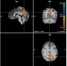
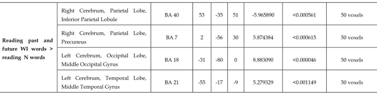
FIGURE 3.10:RFX RESULTS.RELEVANT RECRUITMENT OF PARIETAL LOBULE (BA40) FOR PAST AND FUTURE

CONDITIONS >NEUTRAL CONDITION ... 34 FIGURE 3.11RFX RESULTS.RELEVANT RECRUITMENT OF PRECUNEUS (BA7) FOR PAST AND FUTURE CONDITIONS

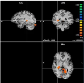
>NEUTRAL CONDITION... 34 FIGURE 3.12:RFX RESULTS.RELEVANT RECRUITMENT OF MIDDLE OCCIPITAL GYRUS (BA18) FOR PAST AND

FUTURE CONDITIONS >NEUTRAL CONDITION ... 35 FIGURE 3.13:RFX RESULTS.RELEVANT RECRUITMENT OF MIDDLE TEMPORAL GYRUS (BA21) FOR PAST AND

FUTURE CONDITIONS >NEUTRAL CONDITION ... 35 FIGURE 3.14:MVPARESULTS.THE INFERIOR PARIETAL LOBULE (BA39) AS A PATTERN OF DIFFERENTIATION

BETWEEN NEUTRAL AND PAST CONDITIONS ... 39 FIGURE 3.15:MVPARESULTS.THE MIDDLE FRONTAL GYRUS (BA9) AS A PATTERN OF DIFFERENTIATION BETWEEN

NEUTRAL AND PAST CONDITIONS ... 39 FIGURE 3.16:MVPARESULTS.THE SUPRAMARGYNAL GYRUS (BA40) AS A PATTERN OF DIFFERENTIATION

(18)

XIV

FIGURE 3.17:MVPARESULTS.THE INFERIOR FRONTAL GYRUS (BA9) AS A PATTERN OF DIFFERENTIATION BETWEEN NEUTRAL AND PAST CONDITIONS ... 39 FIGURE 3.18:MVPARESULTS.THE PRECUNEUS (BA7) AS A PATTERN OF DIFFERENTIATION BETWEEN NEUTRAL

AND FUTURE CONDITIONS ... 40 FIGURE 3.19:MVPARESULTS.THE CAUDATE BODY AS A PATTERN OF DIFFERENTIATION BETWEEN NEUTRAL AND

FUTURE CONDITIONS ... 40 FIGURE 3.20:MVPARESULTS.THE UNCUS (BA34) AS A PATTERN OF DIFFERENTIATION BETWEEN PAST AND

FUTURE CONDITIONS ... 40 FIGURE 3.21:MVPARESULTS.THE PARACENTRAL LOBULE (BA5) AS A PATTERN OF DIFFERENTIATION BETWEEN

PAST AND FUTURE CONDITIONS ... 40 FIGURE 7.1:SLICE SHIFTING DURING SLICE SCAN TIME CORRECTION FOR SLICES THAT WERE ACQUIRED

SEQUENCIALLY (A) AND INTERCHANGEABLY (B).(IMAGE COLLECTED FROM BRAINVOYAGER'S USER GUIDE)63 FIGURE 7.2:RIGID BODY MOTION PARAMETERS PLOT SHOWN AUTOMATICALLY BY BRAINVOYAGER AFTER HEAD

MOTION DETECTION AND CORRECTION (IMAGE COLLECTED FROM BRAINVOYAGER'S USER GUIDE) ... 65 FIGURE 7.3:EXAMPLE TIME COURSE THAT SHOWS THE VARIATION IN SIGNAL’S DRIFT BEFORE AND AFTER REMOVAL

OF LINEAR AND NON-LINEAR TRENDS.THE BLUE CURVE REPRESENTS THE ORIGINAL DATA, THE GREEN LINE IS THE FIT OF THE GLM AND THE MAGENTA CURVE CORRESPONDS TO THE FILTERED RESULTING DATA (IMAGE COLLECTED FROM BRAINVOYAGER'S USER GUIDE) ... 68 FIGURE 7.4:TALAIRACH TRANSFORMATION’S 3D CUBOID REPRESENTATION (IMAGE COLLECTED FROM

BRAINVOYAGER'S USER GUIDE) ... 69 FIGURE 7.5:REPRESENTATION OF BIAS FIELD ESTIMATION AND FINAL RESULT OBTAIN WITH BRAINVOYAGER’S

AUTOMATIC INTENSITY INHOMOGENEITIES CORRECTION (COLLECTEC FROM BRAINVOYAGER QX USER GUIDE) ... 73 FIGURE 7.6:INITIAL 3D ANATOMICAL DATA (LEFT SIDE) COUNTERPOSED WITH THE 3D ANATOMICAL IMAGE

OBTAINED AFTER INTENSITY INHOMOGENEITIES CORRECTION WITH BRAINVOYAGER’S AUTOMATIC TOOL

(19)

XV

List of Tables

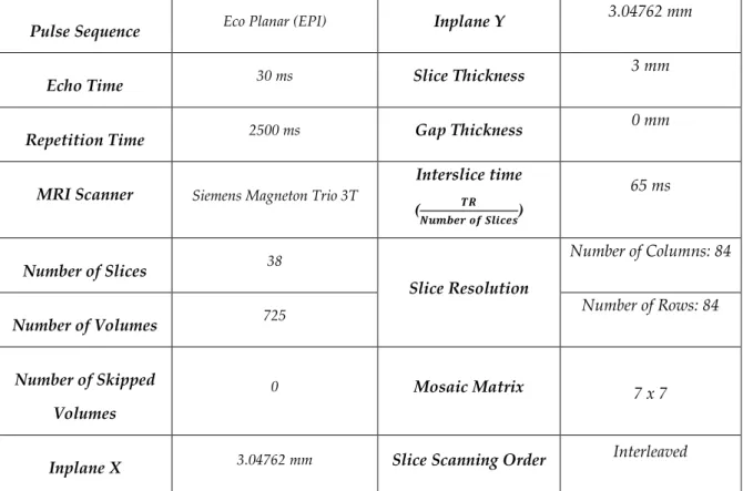
TABLE 2.1:FUNCTIONAL MAGNETIC RESONANCE IMAGING ACQUISITION PARAMETERS ... 21

Table 2.2: ANATOMICAL MAGNETIC RESONANCE IMAGING ACQUISITION PARAMETERS……….21

TABLE 3.1:RFXTALAIRACH COORDINATES TABLE WITH T-VALUES, P-VALUES AND CLUSTER THRESHOLD FOR MULTIPLE COMPARISONS CORRECTION ... 36 TABLE 3.2:FFXTALAIRACH COORDINATES TABLE WITH T-VALUES, P-VALUES AND Q(FDR) VALUE FOR MULTIPLE

(20)

(21)

1

1 State of the Art and Motivation

1.1)

Neural Correlates of past/present events retrieval and future

envisioning

The ability to mentally simulate an episode is common to every healthy human being. This remarkable capability allows us to remember and vividly represent, within our own imagination, personal events that occurred in the past. Moreover, it allows us to envision the outcomes of a possible future situa-tion.

Mental imagery is thought to be granted mainly by a wide archive: our memory system. We recollect pieces of information that combined form coher-ent represcoher-entations of differcoher-ent evcoher-ents. This recombination may be more or less flexible depending on whether we are attempting to envision something that may occur or simply trying to remember something that has already happened. Either way, since the archive is the same, various neuroscientists believe that past recollection and episodic future thought have the same neurologic basis and serve as complementary functions at one’s ability to mentally travel over time (Szpunar et al. (2006), Botzung et al. (2008), Andrews-Hanna et al. (2014)).

Several studies have been performed in which subjects were asked to talk about or just imagine past, present or future events while undergoing neu-roimaging exams such as Positron Emission Tomography (PET) (Okuda et al.

(22)

2

(2003)) and Functional Magnetic Resonance Imaging (fMRI) (Szpunar et al. (2006), Addis et al. (2007), Botzung et al. (2008), Viard et al (2010)). The great majority of these studies were, in fact, able to identify brain areas that seemed to be recruited equally while envisioning past and future events.

Mentally constructing an episode (independently of its associated time-stamp) appears to involve the activation of brain areas situated mainly in the medial posterior cortex and the medial temporal lobe (Okuda et al. (2003); Szpunar et al. (2006); Botzung et al. (2008); Addis et al. (2007); Andrews-Hanna et al. (2014)) and some parts of the left hippocampus (Addis et al. (2007)). More specifically, the right inferior parietal lobule (BA 39 and 40), left superior occipi-tal gyrus/cuneus (BA 18) and right middle occipioccipi-tal gyrus (BA 19) (Addis et al. (2007)) showed similar patterns of activation during past recollection and future

imagining. The medial surface of the temporal lobe forms a system of structures

thought to be mainly concerned with memory, with special emphasis to de-clarative memory (conscious memory for facts and events). The hippocampus is an important part of this system and seems to have an important role in com-bining information from multiple sources (for instance, while recollection of specific events from the episodic memory system). The noted existence of high-ly similar patterns of brain activation involved in both future and past episodic construction corroborated the idea that the ability to mentally travel along the

axis of one’s own subjective time can only be possible through the act of

com-bining and recomcom-bining basic mnemonic elements to generate a complex men-tal image. In that case, the temporal areas recruited would be responsible for the recollection and recombination of memory elements to form an event, while the visual processing areas (BA 18 and 19) would be involved in the construc-tion of the event’s mental representaconstruc-tion (Addis et al. (2007)). As the parietal areas recruited were reported to be mostly concerned with attention, their func-tion in memory may involve orienting attenfunc-tion to internal memory representa-tion (Addis et al. (2007)).

(23)

3

et al. (2008); Addis et al. (2007); Andrews-Hanna et al. (2014)). Past and future elaborations were shown to have the same level of activation in the autobio-graphic memory network, which is composed by frontopolar (BA 10) and infe-rior (BA 11) aspects of the left medial prefrontal cortex, left temporal pole (BA 38) and middle temporal gyrus (BA 20/21), left hippocampus, bilateral parahippocampal gyrus, bilateral posterior cingulate (BA 29, 30 and 31), left precuneus (BA 7), bilateral anterior parietal lobule (BA 39) and cerebellum (Addis et al. (2007)).

Once studies suggest preferential recruitment of the prefrontal cortex for self-referential mental activity, it is plausible to hypothesize that, in order to generate plausible images of the past or future one must reactivate images pre-viously kept in the posterior cortex (Szpunar et al. (2006); Addis et al. (2007)) Furthermore, the involvement of both prefrontal and posterior subsystems in autobiographical tasks reinforces the hypothesis that episodic retrieval and mentalizing play an important role in recalling one’s past and imagining one’s future.

On the other hand, researchers were able to identify some areas more po-tentially involved in extracting future prospects than collecting past experiences during construction and elaboration of metal episodes. In the construction phase, the differentiation of past and future were maximal (when compared with the elaboration phase) with prevalence of the future envisioning. The brain regions recruited during construction were right hippocampus (Okuda et al. (2003); Addis et al. (2007)), right hemispheric BA 10 and left BA 11 from the frontopolar cortex (Okuda et al. (2003); Addis et al. (2007)), and some motor ar-eas such as lateral premotor cortex, medial posterior parietal cortex and poste-rior cerebellum (Szpunar et al. (2006)). The posteposte-rior right middle temporal gyrus and left inferior parietal lobule were greatly activated in the elaboration of future thought (Addis et al. (2007)).

(24)

4

events recollection might be associated with greater self-involvement when compared with episodic future. From this perspective, the act of reflecting about an experienced personal event involves more details, thoughts and feel-ing associated than just imaginfeel-ing somethfeel-ing that has not even occurred yet.

Considering the reviewed literature, we might suggest that there are two major lines of results across studies: one defending that envisioning the future encompasses more intense recruitment of certain brain regions (Okuda et al. (2003), Addis et al. (2007), Szpunar et al. (2006)); and another which states that recollecting and reflecting on past episodes require greater amount of activation in certain cerebral (Botzung et al. (2008)). Several factors may underlie this fun-damental controversy such as, for instance, the chosen experimental paradigm or the imaging method itself.

We resort to recollection of past events and envision of future episodes on a regular basis, countless times a day, intentionally or not. In fact, the human brain is thought to have a certain amount of activity at any given time, even when an individual is at a resting state. When the brain is at a wakeful rest, studies have shown that its default mode network is always active, performing task-independent introspection. Moreover, recent researches about these self-referential thoughts that characterize the resting brain have been able to link them with associative processing involving recollection of past/present memo-ries and envisioning the future.

This nearly permanent mental travelling is often engaged when we

wor-ry about some event from our everyday life. For instance, when we don’t feel

comfortable about something that has occurred, or when we feel anxious about a future situation.

Since worrying involves mainly self-referential negative thoughts and is evermore related with past or upcoming events, it is plausible to foresee that different time-related types of worrying will incite the activity of different brain regions.

(25)

5

Worrying is a relatively common feeling, experienced in a great variety of situations, pathologic or not. It characterizes anxious apprehension (the mildest type of anxiety that seems to underlie the worrying states) and encom-passes repetitive thoughts which may be related to personal and emotional threats to self, competence at work or general world problems (Engels et al. (2007)). Worrisome thoughts appear to constitute an attempt to prevent or min-imize negative emotions related to unpleasant images (Hofmann et al. (2005)). Furthermore, the worrying state is associated with conscious exaggerated threat appraisal and is thought to encompass negative estimates of distant, uncertain and unpredictable dangers that may accrue from either self-relevant aspects or external threats (Kalisch et al. (2014)). When a self-related thought is generated, the anxiety and negative emotionality experienced escalate rapidly and tend to be maintained for long periods of time (Kalisch et al. (2014)). Berenbaum et al. (2010) created a detailed two-step initiation-termination model to characterize the process of worrying. According to him, in an initial phase, the worrying state is generated when an individual perceives a threat and becomes aware of its potential undesirable outcome. Intuitively, the greater the threat, the more likely is worrying to be initiated. The second phase of this model, the termina-tion phase, involves the acceptance of the prospect of the threat. Accepting the inevitability of a danger or risk seems to provide a certain sense of closure to the worrying individual and terminates his anxiety state.

According to important studies onto this subject, anxious apprehension involves mostly verbal and cognitive components and is characterized by larger frontal asymmetry in favor of the left hemisphere (Hofmann et al. (2005); Engels et al. (2007)).

(26)

6

gyrus (BA 10) and the anterior cingulate cortex (BA 25). Overall, for both audi-tory and visual stimuli that induced worry, their research allowed the identifi-cation of several worry-related brain areas, most of which medial regions of the frontal lobe. These findings were particularly interesting because the spotted

areas are thought to be related to reflection of one’s own mental state and on

mental states of others.

(27)

7

Some individuals have an unusual tendency to worry, which means they may find it difficult to perform the cognitive tasks that allow them to terminate the process of worrying. In some cases, this tendency is so overwhelming that ultimately gives rise to psychiatric disorders such as Depression, Obsessive Compulsion Disorder (OCD) and, specially, General Anxiety Disorder (GAD) (Davey and Wells (2006)).

Studying and understanding this type of emotional states is highly

im-portant, not only because they are common aspects of almost all individuals’

lives but because of the important role they play in many forms of psycho-pathology.

1.3)

Clinical Applications

Anxiety disorders have been studied using functional imaging tech-niques. As they are highly common psychiatric disorders (Garner et al. (2009), Moreno-Peral et al. (2014)), understanding and characterizing them at neuronal levels may contribute to more adequate medical treatments and therapies. The central symptom shown by patients with psychopathologies such as General Anxiety Disorder is worry (Paulesu et al. (2010)). Some studies, that compare subjects with generalized anxiety disorder (GAD) and normal controls, have shown that in both groups the same brain region usually undergoes activation during worrying thoughts (Paulesu et al. (2010), Andreescu et al. (2011)). In GAD patients this activation tends to extend itself over time, even during relax-ation phases, which suggests that GAD subjects may have an inability to recog-nize the moment in which it would be useful to stop worrying (Paulesu et al. (2010)).

(28)

8

Spin Labeling perfusion MRI spotted a lack of recruitment of certain prefrontal cortical areas responsible for worry suppression in elderly GAD subjects (Andreescu et al. (2011)). This evidenced that pathologic worry may be associ-ated with a greater difficulty in successfully stopping brain’s processes i n-volved in worrying.

1.4)

Motivation

The present study will focus on the identification of brain areas recruited while normative subjects read sentences related to past/present or future wor-ries. Our main aim is to accurately characterize these brain areas in normal conditions while providing them with a time-stamp that would hopefully help us understand the implications of past/present memories and future envision-ing in worryenvision-ing episodes. With that purpose blood-oxygen-level dependent (BOLD) signals will be collected within a healthy population sample using functional magnetic resonance imaging (fMRI).

1.5)

Functional Magnetic Resonance Imaging: An Overview

The information on the present subchapter is based upon Scott A. Huettel

and colleges’ textbook: “Functional Magnetic Resonance Imaging”; chapters 1,

6, 7 and 8.

(29)

9  Basic Principles

Neuronal activity requires oxygen which is transported by blood’s

he-moglobin throughout the circulatory system. Therefore, in brain’s activated ar-eas, the oxygen consumption rate is higher than normal which triggers body’s compensatory mechanisms to increase blood flow and, consequently, oxygen supply in the area. Since these compensatory mechanisms often exceed the re-quirements, the increasing blood flow leads to an abnormal augmentation in oxygenated hemoglobin’s (Hb) concentration in the activation area. Additional-ly, the concentration of deoxygenated hemoglobin (dHb) in the same area will be unusually low. Consequently, Hb/dHb ratio will increase which seems to characterize neuronal activity.

Deoxygenated hemoglobin has paramagnetic properties responsible for the generation of microscopic magnetic fields within the MR scanner, causing heterogeneities in the main magnetic field. However, the decreasing proportion of dHb during activation counteracts those heterogeneities, increasing tissues’

characteristic real transverse relaxation time, T2*. Using MRI T2* contrast

tech-niques, it is possible to identify significant increases in signal’s intensity in brain activation regions, which become localizable.

 Blood–Oxygenated–Level Dependent Technique (BOLD)

Several fMRI studies, including the present one, use a blood-oxygenation-level dependent technique (BOLD). This approach takes into consideration the increasing signal in brain regions with high Hb/dHb ratio to find presumable

cerebral activations with resort to T2* contrast techniques. We assume that the

(30)

10  Hemodynamic Response Function (HRF)

Generally, for a short stimulus, HRF may be represented by Figure1.1.

In Figure 1.1, the decrease in signal verified immediately after the stimu-lus (“initial dip”) is due to the sudden increase in oxygen consumption when neuronal activity is initiated. Shortly after, once the compensatory mechanisms take action, BOLD signal increases, thus forming the function’s peak.

With the end of the stimulus, neuronal activity ceases and other compensatory mechanisms are stimulated this time in order to guarantee the diminution of local blood flow. As a consequence, BOLD signal decreases. The “negative overshoot” present in Figure 1.1 evidences the exaggerated vessel constriction (an effect of the compensatory mechanisms) which leads to an abnormally low-er Hb/dHb ratio. Body’s compensatory mechanisms take some seconds to reestablish normal blood flow (BOLD signal’s baseline).

In conclusion, it should be noted beforehand that BOLD fMRI does not recognize neuronal activity per se, but the metabolic demand of active neurons.

1.6)

Methods for Statistical Analysis of fMRI data

Neuroimaging studies using fMRI give rise to massive amounts of data with its unavoidable noise and artifacts derived from countless sources. Hence, statistics play a crucial role in understading the nature of the data and accessing

(31)

11

its relevance, providing neuroscientists with important interpretational infor-mation. In this chapter we will illustrate interesting and important issues in which statistics are critical for fMRI data manipulation.

 Single Subject Analysis

In order to truly understand the nature of BOLD signal, and, specially, to localize brain activity, it is essential to establish three background assumptions. First of all, the signal provides a measure of the amplitude of neuronal activity under a certain condition. This implies that fMRI signal will be scaled by a fac-tor if the input (the neuronal activity) is scaled by the same facfac-tor. Secondly, fMRI signal is cumulative, i.e. the response to two different stimuli applied to-gether equals the sum of the individual responses to each stimulus individu-ally. And, finally, when a stimulus is shifted by a time t, the response is also shifted by t, hence, fMRI signal is time-invariant. All previously mentioned as-sumptions form the baseline from which it is possible to start handling fMRI data and, hopefully, draw meaningful conclusions. Namely, distinguish be-tween highly and slightly activated brain areas, and discriminate data from dif-ferent conditions.

In the present work, the method used to single subject’s fMRI statistical analysis is the General Linear Model (GLM).

The General Linear Model

The general linear model is the univariate statistical method (introduced in the neuroscience community by Friston et al. (1994)) that underlies most fMRI data analysis. It is a multiple regression technique which evaluates the relative contributions of all processes that may be involved in the generation of

the observed data, yi. Since GLM assumes that both stimulus function and

Hemodynamic Response Function are known a priori, the referred processes,

also known as predictors, may be written in a reference function, Xij, obtained

(32)

12

noise is present within each voxel, an error or residual function, ei, must also be

built. Since each predictor has different quantitative contributions to the

ob-served data, they are associated with individual weighting factors, βj.

The ultimate purpose of the GLM analysis is to find the predictor’s weighting factors that best accounts for the original data by minimizing the er-ror or residual terms. The following equations represent the linear correlations performed in this regression technique:

…

Equation 1.1

The weighting of each physiologic parameter as well as the error terms are

calculated for each voxel independently. The first β value, β0, typically

repre-sents the signal level of the baseline condition.

The physiologic processes’ hypothesized changes over time (as a result of the different stimuli underwent by the subjects during the fMRI scanning), re-lated to the expected hemodynamic response in time, may also be represented

in a design matrix, G, with n rows (number of hemodynamic peaks during the

entire scanning) and M columns (number of physiologic processes). On the

other hand, as the noise is present within each voxel, the error matrix, ε, will

also have n rows but V columns (the number of voxels in the imaging volume).

The time evolution of the fMRI data is also arranged in a two-dimensional

ma-trix with n rows and V columns and is known as the data matrix, Y. Finally, the

weighting factors form the parameter matrix, β, with V rows and M columns

(33)

13

Equation 1.2

GLM’s residual time course typically exhibits serial correlations, i.e. high values followed more likely by high values than low values and vice versa. Se-rial correlations violate the assumption of uncorrelated errors, and probably oc-cur due to the rapid succession of data point’s measurement. However, since GLM expects the original voxel time course to present this type of biased in-formation, its correction is done effectively during this statistical operation. Therefore, the estimated beta values are unbiased. Nevertheless, the standard errors of beta values are biased resulting in an abnormal increase in t-values

ob-tained.In order to avoid this sort of errors, it is possible to correct serial

correla-tions using a pre-whitening approach in which autocorrelation is estimated by assuming the errors follow a first-order autoregressive, or AR(1), process. In this approach, GLM is calculated normally, subsequently estimating the

amount of serial correlations, r, using a pair of successive residual values (the

time course of a certain residual is correlated with itself shifted by one time

point). Measured voxel’s time course (yt) is then re-adjusted and a transformed

time course (ytn) is calculated by removal of the estimated r values (as can be

seen in Equation 1.3)

Equation 1.3

The design matrix is re-adjusted as well by applying the same calculation to each predictor’s time course. Finally, correct standard errors for beta

esti-mates and correct significance levels (t-values) are obtained by re-computation

of the GLM using the corrected voxel time courses and the adjusted design ma-trix.

(34)

14

does not provide information about absolute levels of brain activation. Instead it represents the changes in activation over time. Therefore, it is necessary to compare activation between two or more experimental conditions by statistical evaluating if the experimental alterations evoke significant changes in the over-all cerebral activation. This evaluation is cover-alled contrast, and it may be in rela-tion to baseline activity or between experimental tasks.

Although simple, GLM represents a powerful and rigid approach to-wards modulating data. However, due to the massive amount of data, examin-ing the appropriateness of the model is challengexamin-ing and standard methods of model diagnostics are not feasible.

 Group-Level Analysis

So far we have focused on the statistical methods to identify areas of ac-tivation within a single subject’s brain. However, the majority of fMRI research (the present study included) fundamentally aim to identify the recruited brain areas in a certain experimental condition and generalize their activation within a sampled population (with specific features that characterizes the group). Nonetheless, combining data from multiple subjects presents more than a few challenges, which is why it is important to choose the more adequate statistical approach for intersubject analysis.

The main two statistical methods for multisubject fMRI data analysis are: Fixed Effects Analysis (FFX) and Random Effects Analysis (RFX).

Fixed Effects Analysis

(35)

15

This method offers great sensitivity and statistical power, thus present-ing a popular way to analyse intersubject fMRI data. However, when exclu-sively used, it fails to provide information applicable to the general population, implying that the obtained results are strictly valid only for the investigated group. Intuitively, that happens because when choosing to resort to an average approach, one may be neglecting some subject’s pieces of information substan-tially different from the majority of the data, thus resulting in misleading con-clusions.

Random Effects Analysis

In order to be able to generalize the data to the population from which the sample of subjects have been drawn, a random effects group analysis has to be performed. This statistical approach explicitly models the inter-subject vari-ability by considering each subject merely as one of the many possible partici-pants who could have taken part in the experiment.

Although FFX is a highly sensitive method due to its substantially greater amount of considered degrees of freedom, RFX is a much more appro-priate model to achieve relevant and credible results.

The Multiple Comparisons Problem

During the massive amount of statistical tests performed during fMRI data analysis, there are thousands of voxels that end up by showing statistical significance by chance (positives). The increase in the number of false-positives, also known as family-wise errors, results from increasing number of statistical tests and is known as Multiple Comparisons Problem.

(36)

16  Multi-Voxel Pattern analysis

Unlike GLM, in which a condition effect is analyzed voxel by voxel, the Multi-Voxel Pattern analysis (MVPA) allows the collective analysis of individu-al voxels within a region. MVPA methods offer higher sensibility in detecting and comparing different activation patterns between conditions. These tools are often referred to as classifiers or “learning machines” since they are capable of analyzing a set of fMRI activity patterns that may describe specific mental states and classify them within a finite group of possibilities. Obviously, the classifica-tion process in not random and must follow certain rules which are built in MVPA’s “learning phase”. At this point, fMRI data is divided in two sets. One “training” set used to estimate conditions that provide the match between brain activation patterns (input) and the corresponding class labels (target), thus providing a mapping function of the brain (a vector with N elements, in which each element specifies the presence of a certain feature measured within each one of the N voxels included in the analysis); and another “test” set which will be classified (one previously defined label will be assigned to each new fMRI activation pattern) using the created mapping function. At the end of the learn-ing phase, the classifier should be able to correctly classify new submitted data, as well as the learned and tested activity patterns.

Searchlight Mapping

Since each activation pattern used during the learning phase is represented as a feature vector with N elements, for whole-brain mapping, a great number of activation patterns with high N must be used as learning set, thus resulting in low generalization accuracies because of the large amount of "noise" voxels (those voxels whose activation is not relevant). In order to surpass this problem, classifiers are often deduced from voxels of an anatomically or functionally de-fined region-of-interest (ROIs), generating a multivariate brain mapping.

(37)

17

neighbourhood. The amount of considered voxels in the so called neighbour-hood is defined by the size of a sphere, i.e., a nearby voxel is considered to be-long to the visited voxel’s neighbourhood if it is located at a certain Euclidean distance (less than or equal to the sphere’s radius). The result of the

multivari-ate analysis (the t value resulting from a multivariate statistical comparison)

(38)

(39)

19

2

Methods

2.1)

Data Acquisition

 Participants

Functional Magnetic Resonance data was acquired from ten right-handed volunteers, with ages between 24 and 47 (mean age 32,3 ± 8,31 years). All of them had never been diagnosed with psychiatric or neurologic disorders or any kind of chronic condition. Further, none of the ten participants reported to re-sort to regular medication due to other health problems.

Prior to the acquisition date, the subjects were asked to generate three different written lists, each one containing fifteen groups of two or three words. Two of them had to be filled with words concerning personal past or present and future worries, separately. The third one contained groups of words whose emotional significance is irrelevant to the subject at that time. A feeling-in document with the necessary instructions were delivered to each subject in or-der to assist and ease their participation. Additionally, participants read and signed a confidential Inform Consent approved by the local ethics committee (Comissão de Ética da Faculdade de Medicina da Universidade de Coimbra), which contained important information about the study’s motivation, proce-dures and its possible benefits and risks.

(40)

20

 Task and Experimental Design

The type of fMRI experimental design used is called Blocks design. It is characterized by more extended time intervals for each condition which will lead to a larger evoked response during each task, thus increasing the separa-tion in signal between blocks, ultimately leading to higher detecsepara-tion power.

Once in the MRI Scanner, subjects were confronted with their personal previously written words. Each word appeared for 2s in a screen and the par-ticipants were asked to read and reflect about it. Every type of word was sepa-rated in three different condition blocks of 30s (neutral, past/present worrying or future worrying), each of which repeated ten times over the course of data acquisition. Intercalated with the conditions blocks, there was also a 30s-lasting resting block during which participants were asked to fixate a cross that

ap-peared in the centre of the screen.

A simplified representation of our block design paradigm is portrayed in Figure 2.1.

 MRI Acquisition Parameters

(41)

21

The main acquisition details of anatomical and functional image’s acquisi-tion are listed in Table 2.2 and Table 2.3, respectively.

Image Resolution

Number of columns: 256 Slice Thickness 1 mm

Number of rows: 256

Spacing Between

Slices

0 mm

Pulse Sequence MPRAGE

Repetition Time 2530

Number of Slices 176

Pulse Sequence Eco Planar (EPI) Inplane Y

3.04762 mm

Echo Time 30 ms Slice Thickness

3 mm

Repetition Time 2500 ms Gap Thickness

0 mm

MRI Scanner Siemens Magneton Trio 3T

Interslice time

( )

65 ms

Number of Slices 38

Slice Resolution

Number of Columns: 84

Number of Volumes 725

Number of Rows: 84

Number of Skipped Volumes

0 Mosaic Matrix _{7 x 7}

Inplane X 3.04762 mm Slice Scanning Order Interleaved

Table 2.1: Anatomical Magnetic Resonance Imaging acquisition parameters

(42)

(43)

21

2.2)

Data Processing

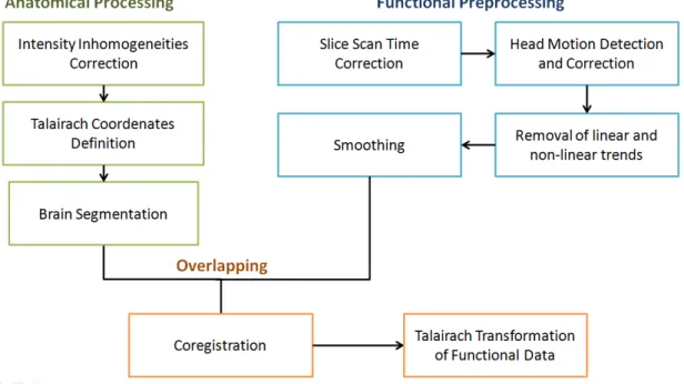
Because both functional and anatomical raw images may not be perfectly aligned (due to subjects’ movements) and may exhibit scanning artifacts, sim-ply overlapping them may provide erroneous results. Therefore, both anatomi-cal and functional images must be processed separately before coregistration.

The scheme portrayed in Figure 2.2 shows the various steps taken throughout data processing in this particular work.

All data handling were performed using the software package

BrainVoy-agerQX 2.8. The following described information about the processes and

meth-ods to image processing and statistical analysis are featured in Brainvoyager’s

Support website.

(44)

22  Anatomical Data Processing

Intensity Inhomogeneities Correction

First of all, contrast and brightness were adjusted manually in order to obtain grey matter intensities of approximately “100” and white matter intensi-ties around “160”, providing the best grey-white matter separation possible and allowing a proper visualization of the brain cortex.

Since during data scanning the inhomogeneities of the applied magnetic fields may induce artifacts in the acquired anatomical images, the first move in anatomical data processing must be intensity inhomogeneity correction (IIHC). The software offers an automatic tool that executes IIHC without user’s inter-vention. This tool performs image’s background cleaning and erosion, detection of white matter and bias field estimation (see detailed steps in Appendix 7) to generate a new 3D anatomical image whose voxels have much more homoge-neous intensities (grey matter intensities will be centred around intensity “100” and white matter intensities around “160” by default). IIHC improves anatomi-cal data’s visualization and creates better starting points for subsequent seg-mentation tools.

Talairach Coordenates Definition

Due to anatomical variability across subjects, it is very important to de-fine a common coordinate space in which both structural and functional images

can be overlapped. The most commonly used standard space is called the

Ta-lairach space and is obtained by submitting both anatomical and functional data

to a Talairach transformation. Talairach coordinates are defined directly in the

structural data, through manual identification of specific anatomical regions.

For more detailed information about Talairach transformation see Appendix 6.

Brain Segmentation

(45)

23

mesh. Brain segmentation is essential for volume or surface rendering, as well as for precise estimates of cortical thickness. In the present study, brain segmen-tation allowed us to build a mask of the cortex which was, posteriorly, used in the multi-voxel pattern analysis technique further discussed (see subchapter 2.5).

BrainVoyager QX provides an automatic cortex segmentation tool, in

which a series of steps are sequentially performed until the 3D reconstructed structure is finally delineated (see Appendix 2).

 Functional Data Preprocessing

Following anatomical image reconstruction and in order to prepare the statistical analysis, it is important to remove artifacts and confound variability from the acquired functional data. For that, we resort to a series of

computa-tional processes that are collectively called preprocessing. BrainVoyager QX has

in-built functions, however it is important to understand all steps in order to guarantee accurate results.

Slice Scan Time Correction

Slice scan timing correction is applied to eliminate the time-variability be-tween scanned slices (not all brain regions are scanned at the same moment in time) that could lead to suboptimal statistical analysis. To achieve temporal alignment amongst slices, each slice’s data is shifted in time from its original scan time point to match the same time point as when a reference slice (the first

slice of the functional volume in our case)was acquired (see Appendix 3). With

this purpose, the software relies on information from the defined acquisition protocol.

All shifted slices must undergo changes in data in order to better represent the information that would have been recorded if the original time point coin-cided with the reference. In our study, the estimation of new voxel intensity

values was accessed using a sinc interpolation. This method offered a better

(46)

24

Head motion detection and correction

Since the most common artifacts come from subject’s head movements

within the scanner, BrainVoyager QX also counts with a standard optimization

algorithm that enables the correction of head movement by coregistrating suc-cessive image slices to a single reference one (in this case the first scanned slice) using, once more, a combination of three translations and three rotations (see Appendix 4).

As a final step, to gauge new volume’s signal values whose position fall

in-between measured data points, we resort to trilinear sinc spatial

interpola-tion. This interpolation method achieves the highest quality results, i.e. gives rise to corrected functional volumes that reflect the original data as closely as possible.

Removal of Linear and non-linear trends

Linear and non-linear trends correction is also a very important preproc-essing step, since it allows the removal of low-frequency drifts caused normally by physiological noise (heart beat, breathing and others) or physical noise (from the MRI scanner) that would decrease substantially the power of statistical data analysis. These low-frequency drifts are removed through the application of a high-pass filter in each individual voxel’s time course. In general, high-pass fil-ters remove low-frequency portions of a signal (the drifts in this case) while preserving the high-frequency ones.

(47)

25

Spatial and Temporal Smoothing

Temporal and spatial filtering may also be used to perform the smooth-ing of the acquired image. The advantages of smoothsmooth-ing are: improvsmooth-ing of sig-nal-to-noise ratio, reducing high-frequency spatial components and, most im-portantly, easing group analysis by improving inter-subject registration and overcoming limitations in the spatial normalization by blurring any residual anatomic differences. A mean smoothing filter of 8 mm Full Width Half Maxi-mum was applied to this study’s data as the last step of the preprocessing of functional information.

 Overlaying Functional and Anatomical data

Coregistration

The coregistration of functional and anatomical data sets is performed automatically by the software, upon previous indication of the chosen strate-gies. It may be divided in two main steps: an initial alignment (IA) followed by a fine-tuning alignment (FA).

In this study’s particular case, since anatomical and functional data are both recorded in the same session and in a file format containing the required positioning information, an IA with resource to header-based coregistration will be performed.

(48)

26

Talairach Transformation of Functional Data

In order to assure a reliable and precise interpretation of the functional results given by coregistration, functional data must also be converted into the

Talairach space. BrainVoyager Qx is able to perform the Talairach transformation

of the functional data automatically, with resource to several pieces of informa-tion produced in previous steps: the preprocessed funcinforma-tional image, both IA and FA alignments of anatomical and functional data, AC-PC translations and rotation performed and cerebrum borders defined. By linking the transformed functional and anatomical data, we obtain an aligned and normalized image containing a 4D data set: 3D space x 1D time.

2.3)

Single Study Statistical Analysis

So far we have both anatomical and functional data converted into

Ta-lairach coordinates system and ready for statistical analysis. The first

re-comended stage of fMRI statistical analysis encompasses the examination of each subject’s data separately, in order to ascertain that all preprocessing stages were successfully implemented.

In our study, we opted to apply a General Linear Model to each subject’s

preprocessed functional data to create the statistical maps of all brain areas re-cruited during each one of the different conditions of the experimental para-digm.

 The General Linear Model (GLM)

As seen so far, the GLM aims to predict the variation of the observed fMRI time course of a voxel for different conditions with respect to the expected time course of a theoretically idealized hemodynamic response function.

(49)

27

BrainVoyager QX automatically identifies the main GLM predictors (three,

one for each condition excluding the resting state) using the previously defined protocol. In addition, we introduced six new parameters (generated from the resulting file from 3D motion correction), one for each translational and rota-tional rigid movement imposed to the funcrota-tional data during detection and cor-rection of head movements. This will allow controlling for the effect of motion in possible creation of false positives.

In this project, we performed serial correlations correction using

Brain-Voyager QX’s AR(1) process (explained in subchapter 1.6).

Since GLM is performed independently for each voxel’s time course, the result of its statistical operations will be a set of estimated beta values attached

to each voxel. Resorting to a %-Transform, it was possible to obtain

voxel-specific statistical values (t and p) for a specified contrast (comparison between two different tasks from the experimental protocol) using each voxel’s vector of betas as an input. The estimated t and p values are then collected in a 3D data set known as statistical map. This map will show the estimated statistical values

at the position of each corresponding voxel in the Talairach transformed

func-tional data. By establishing specific minimal and maximal thresholds that must be or not exceeded by voxel’s functional intensities, respectively, it is possible to overlap the statistical map to a 3D anatomical image and visualize only p and t values of functional voxels with statistical significance while still seeing ana-tomical information as the background. The final 3D image obtained will show anatomical information in a grey colour scale, and statistically relevant func-tional information in a multiple colours scale, using red-to-yellow colour range for positive values and a green-to-blue colour range for negative values. Ulti-mately, it will be possible to analyse and localize with relative precision (due to the fact that both anatomical and statistical map are in the same coordinate

sys-tem – the Talairach space) the brain areas exhibiting significant signal

(50)

28

2.4)

Group-Level Statistical Analysis

 Fixed Effects (FFX) Group Analysis with False Discovery Rate (FDR)

In this study, the intersubject analysis was initialized by combining all data points from all subjects into a single analysis, using Fixed Effects Group Analysis. We saw that FFX assumes that the effect of the experimental manipu-lation is fixed across subjects, with possible differences between subjects caused by random noise.

BrainVoyager QX’s multi subject analysis tool uses the previously ob-tained single study GLM information to automatically concatenate the data from all subjects and create a multi-study design matrix. Using a z-transformation, the discrete values that integrate the new design matrix are then converted into a complex frequency domain function, and the variance be-tween subjects is normalized. As a result, we obtain a volume map that, when overlaid to an anatomical image, can provide information about which brain areas are activated across subjects persistently during a certain task.

The final volume map must be tested for statistical significance using the more appropriate technique. This technique should allow the overcoming of the multiple comparison problems, while providing relevant results. In our case, for such a small number of participants, the Bonferroni approach did not give any results. Therefore, we opted to use the False Discovery Rate technique, with q-values from 0.01 to 0.05 (see Appendix 1).

 Random Effects (RFX) Group Analysis with Cluster-Level Statistial Thresholding

(51)

29

Usually, RFX operates in two statistical levels: one in which mean effects estimation per condition is performed for each subject; and another which re-ceives the first-level RFX results as independent variables and models their variability across subjects.

In Brainvoyager QX, RFX’s first-level results are a GLM outcome, namely

the set of estimated effects (β values) for each subject undergoing one specific condition. These results are then subjected to one second-level statistical analy-sis method. In our case, we chose to perform an RFX-GLM which operates sub-stantially faster than any other method, and requires much less working mem-ory. With RFX-GLM, a summary statistics approach receives the first-level GLM beta values as input and specifies the same contrast across them, calculating this contrast’s mean value and testing it against zero using a t-test.

Since throughout the RFX-GLM approach the majority of the data was examined separately for each subject, the volume map resulting from this stage of the statistical analysis can be generalized to the population.

Finally, the resulting volume map was tested for statistical significance with a Cluster-Level Thresholding (see Appendix 1). In order to find the

appro-priate cluster size, BrainVoyager QX’s Cluster-Level Statistical Threshold

Esti-mator plug-in, the “ClusterThresh”, was used. Clusterthresh iteratively calculates

the minimum possible cluster threshold via MonteCarlo simulations of the

ran-dom process of image generation. The number of performed iterations at this point was the recommended by the plug-in creators, i.e. 1000 iterations. The plug-in then estimates spatial correlations between neighbouring voxels and their intensities. Finally it identifies the minimum cluster size threshold, which

becomes automatically set in BrainVoyager QX’s volume map options.

2.5)

Multi-Voxel Pattern Analysis (MVPA)

In BrainVoyager QX, MVPA methods are supervised, which means that all

(52)

30

classification of each activation pattern is already known. Thus, some cases of poor generalization performance due to overfitting (the condition of the map-ping function are overly adjusted to the learning set) may be detected.

 Trial Estimation

The training map functions (the conjunction of all feature vectors) for each class is created using a standard GLM whose beta values are estimated (resort-ing to a 2gamma HRF) for each individual trial. As seen previously, the beta values represent the amplitude of the hemodynamic response of relevant voxels at a certain time point. The trial estimation step allows the obtainment of as many training exemplars as possible for each class, by using the estimated betas for each trial per voxel as the trial response values that will integrate the feature

vectors.

 Searchlight Mapping

In the present study, we performed whole-brain multivariate searchlight mapping. The implemented multivariate statistic method to estimate the t-value of each voxel was a Support Vector Machine based (SVM) searchlight with a sphere radius of 2 voxels. Additionally, we created a mask of the cortex to con-fine the search of pattern of activity to grey matter

In both multivariate statistical estimation methods, the activity patterns were examined for two experimental conditions at a time (past and future, past and neutral or future and neutral words).

(53)

31

3 Results

The main outcomes of this study were obtained with resort to

BrainVoyager QX package, version 2.8.

In this chapter, we put forth the more relevant imaging results obtained in the present study. RFX, FFX and MVPA results will also be summarized in

three tables containing the Talairach coordinates of the voxel with greatest

t-value in every single cluster of brain activation or deactivation detected. These tables will also provide information about the anatomical nomenclature of each

recruited brain region, obtained with resort to Talairach Client (Lancaster et al.

(1997) and (2000)). This component of the Talairach Software (available online)

reports Talairach labels for user-defined coordinates.

3.1)

Group-Level Results

Only the relevant imaging results obtained with RFX will be presented (since they are the ones that can be effectively generalized to the population).

The FFX results will only be portrayed in the respective Talairach table.

(54)

32

 Imaging Data from RFX Group-Level Analysis

Brain Areas Recruited for Past Condition > Neutral Condition

Figure 3.4: RFX Results. Relevant recruitment of middle occipital gyrus (BA 18) for Past Condition > Neutral Condition

Figure 3.3: RFX Results. Relevant recruitment of precuneus (BA 7) for Past Condition > Neutral Condition

Figure 3.1: RFX Results. Relevant recruitment of middle temporal gyrus (BA 21) for Past Condition > Neutral Condition

(55)

33

Brain Areas Recruited for Neutral Condition > Future Condition

Brain Areas Recruited for Past Condition > Future Condition

Figure 3.5: RFX results. Relevant Recruitment of supramarginal gyrus (BA 40) for Neutral Condition > Future Condition

Figure 3.6: RFX results. Relevant Recruitment of primary visual cortex (BA 17) for Past Condition > Future Condition

(56)

34

Brain Areas Recruited for Past and Future Conditions > Neutral Condition Figure 3.9: RFX results. Relevant Recruitment of precuneus (BA 31) for Past Condition > Future Condition

Figure 3.8: RFX results. Relevant Recruitment of middle temporal gyrus (BA 39) for Past Condition > Future Condition

Figure 3.10: RFX results. Relevant Recruitment of parietal lobule (BA 40) for Past and Future Condi-tions > Neutral Condition

(57)

35  RFX Talairach Coordinates Table

Contrast Brain Region

Brodmann

Area

Talairach

Coordinates

t-value p-value

Considered Cluster

Thresh-olds x y z