In Part 1 of this paper (Helbig, 1998 - Rev. Bras. Geof. 16 (2–3):103–114) it was shown that a medium consisting of a periodic sequence of layers is, in the long-wavelength approximation, equivalent to a homogeneous compound medium with elastic parameters that are generalized averages of the constituents’ stiffnesses. Though the matrix-algorithm described in Part 1 works with anisotropic constituents, the most interesting application is to layer sequences with isotro-pic constituents, i.e., to transversely isotroisotro-pic (TI) compound media. Part 2 discusses the possibility to obtain information about the (thin-layer) constituents from the properties of the compound medium. Though every periodic sequence of isotropic layers results in a TI medium, the reverse is not true: there are TI media that cannot be ”modeled” by a periodic sequence of isotropic layers. Those that can be modeled can be inverted to layer sequences that result in precisely the observed anisotropy. This inversion is not unique, but it constrains the possibili-ties. The critical tool to determine the possibility of modeling a TI medium is the concept of stability. Unstable compound media –that release energy on being deformed – would not exist. However, for inversion we must insist that not only the compound medium, but also the poten-tial constituents are stable. In preparing a catalog that covers all possible media, instability is the boundary beyond which the calculation becomes meaningless. Inversion means to determine possible causes of the observed anisotropy, ideally the elastic parameters of the constituents and their contribution to the compound medium. This is possible, though under several restrictions: Not all TI media are long-wave equivalent to a periodically layered sequence of isotropic layers. Those that are can be “modeled” by a variety of layer sequences. Every TI medium that can be modeled at all can be modeled by as few as three layers, but the set of all models is a three-parametric manifold. If a TI medium can be modeled by two constituents only, this can be done only in one way, unless the constituents have the same ratio of S- to P-velocity. In that case, the set of possible models forms a one-parametric manifold.
Key words: Elastic anisotropy; Transverse anisotropy; Exploration seismics; Wave
propaga-tion.
LAYER-INDUCED ELASTIC ANISOTROPY
PART 2: INVERSION OF COMPOUND PARAMETERS TO
CONSTITUENT PARAMETERS
K. Helbig
Received April 22, 1999 / Accepted April 15, 2000
Kiebitzrain 84 D 30657 - Hannover
Fed. Rep. Germany [email protected]
*Based on a Conference presentation made at the Second Brazilian Workshop on Seismic Anisotropy, Campinas, SP, Brazil, November 1996
INTRODUCTION
Part 1 of this paper (Helbig, 1998; henceforth Part 1) describes a matrix algorithm that allows to determine the ”compound stiffnesses” of the replacement medium that is, in the long-wavelength approximation, equivalent to a periodic sequence of thin layers. The matrix algorithm works for layers of arbitrary anisotropy, and should have applications in the determination of the properties of industrial laminates like plywood. However, analytical results for constituent layer of low symmetry are too complicated for a general inversion to be attempted.
In the context of exploration seismics, the constituent layers can be assumed to be approximately isotropic, thus the replacement medium is transversely isotropic (TI), with the axis of symmetry perpendicular to the layers. Though depositional planes are not necessarily horizontal, it is assumed for the purpose of this discussion that the axis of symmetry is vertical. In the standard coordinate system of seismic exploration (x- and y-axis horizontal, z-axis downward) such a medium has five elastic stiffnesses. The reliable determination of all five stiffnesses is possible with current technology, e.g, with a combination of standard surface-to-surface seismics with multi-offset VSP observations.
Once the five elastic stiffnesses of a TI medium have been determined, several questions arise:
1. Could the observed transverse isotropy be due to layering, i.e., can the medium be ”modeled” by a periodic sequence of isotropic layers?
That this is not always the case is obvious: according to Eq. 22 of Part 1, the two shear stiffnesses c55 and c66 of a laminated medium are, respectively, the thickness-weighted harmonic and arithmetic averages of the constituents’ shear stiffnesses µi. Thus c55
≤
c66, with the equality sign valid only in case of isotropy. Therefore, any TI medium with c55≥
c66, cannot owe its anisotropy to lamellation with isotropic constituents.The question will be addressed at a more fundamental level further down. As shall be seen, the answer is always unambiguous, either ”yes” or ”no”.
2.If the answer to question 1 is ”yes”, can a physically realizable model be found?
The answer is always yes, if ”physically realizable” is understood to mean that the hypothetical constituents are allowed by the laws of physics, not that they are available as natural or industrial materials. This poses the next question:
3.Can a realistic – or better, a geologically likely – model be found?
The answer is not easy, but the possibilities can be narrowed down. Even such vague information is valuable, since it refers to details below the resolution of the seismic method.
CONDITIONS FOR A TI MEDIUM TO BE
”INVERTIBLE”
The first question was addressed by Backus (1962). An exhaustive discussion can be found in Helbig (1981). It should not be overlooked that the answer obtained is not necessarily the answer the explorationist has in mind: the layer sequence – if it exists – is not unique, so that one needs further information to narrow the set of all sequences that would be compatible with the observations.
General constraints
The discussion is simplified if one considers an elastic medium of a given symmetry as a particular case of a lower symmetry. For instance, isotropy is a particular case of transverse isotropy, thus every isotropic medium has also transversely isotropic symmetry (and simultaneously has tetragonal, orthorhombic, monoclinic, … symmetry). This is in keeping with the concept of ”hierarchical inclusion” (Fig. 1): any medium is triclinic. If the elastic parameters satisfy certain conditions, it can also be classed as monoclinic (orthorhombic, transversely isotropic, isotropic).
With this proviso the pertinent results of Part 1 can be summarized as follows:
• Every sequence of isotropic layers is a long-wave equivalent to a TI medium.
• Every sequence of isotropic layers with identical θ = (vS/vP)2 is a long-wave equivalent to a K-medium.
• Every sequence of isotropic layers with identical µ is a long-wave equivalent to an isotropic medium.
The inverse of the last two statements is also true: for the K-medium this is trivial, since it is defined as the medium that is long-wave equivalent to periodic layering with constant θ. The fact that every medium that is isotropic for wavelengths in the seismic spectrum might on close inspection turn out to be finely layered with constant shear stiffness µ is a reminder that inversions of this type cannot give unambiguous answers, but can only narrow down possibilities.
Figure 1 - Hierarchy of elastic media. All media are triclinic. If for
a medium of a specific symmetry the conditions listed ”below” are satisfied, it belongs also to the next higher symmetry. Layered sequences with isotropic constituents belong to the sub-sequence at lower right (TI–K-medium–isotropy).
It was already mentioned that a TI medium has to satisfy c55 < c66 if it is to be long wave-equivalent to a sequence of thin isotropic layers with distinct shear stiffnesses µ. However, this is not the only restriction. Another observation of significance in this context is that Rudzki’s (1911) fundamental inequality:
(
)(
)
(
13 55)
0, 2 55 33 55 11 2 > − − − − =+
c
c
c
c
c
c
E
(1)holds for all anisotropic media that are long-wave equivalent to lamination of isotropic constituents with distinct shear stiffnesses. This is easily shown for periodic sequences with two constituents only (Postma, 1955; Helbig, 1958). It was shown to hold for any
number of constituents by Berryman (1979) and Helbig (1979).
The significance of this parameter is the following: for E2 = 0, the slowness surface of P-waves is an ellipsoid of rotation (including a sphere as special case), and the slowness surface of SV-waves is a sphere. For E2 > 0 (< 0) the slowness surface of compressional waves lies outside (inside) the ellipsoid, and that of SV waves lies inside (outside) the sphere. If the slowness surface of SV waves has concave parts (corresponding to cuspoidal edges of the wave surface), they are in the vicinity of the axis of symmetry and/or the plane of symmetry for E2 < 0, and centered about an intermediate direction for E2 > 0 (see Fig. 2, and also Fig. 4 of Part 1). Thus no medium with a strictly ellipsoidal P-wave surface and no medium with E2
≤
0 – particularly no medium with a SV-wave front with cusps near the axis of symmetry or near the plane of symmetry – can owe its anisotropy solely to lamination of isotropic constituents.Stability constraints
Further restrictions are due to the requirement that the effective medium and the constituents are stable. Stability of a medium is generally taken for granted: Any instable medium – i.e., one that releases energy under deformation – would have self-destructed at the slightest provocation. However, if a compound medium is inverted to a layer sequence, one must be certain that also the constituents so determined do not violate the stability constraints.
The condition that any strain results in an increase of the internal energy is equivalent to the condition that all ”leading minors” are positive, for instance, for a strain that has the non-zero components ε3 and ε4. The energy-density P connected to this strain is:
( )
(
)
. . . . . . . . . . . . . . . . . . . . . . . . . . . . . . . . c C c P P T i j ij i iC
• • • • + + = ⇒ = = = 44 2 4 34 4 3 33 2 3 4 3 2 2 1 0 , 0 , , , 0 , 0 2 1 2 1 ε ε ε ε ε ε εε
ε
ε
σ
(2)For the quadratic form in the parenthesis to be positive for any value of the two strain components, it is necessary and sufficient that the determinant of the sub-matrix (the ”minor” corresponding to the particular
Transversely Isotropic Constituents τ σ− = − − − + − = c c c c c c c c k 33 13 33 66 11 33 2 13 66 2 1 4 4 1 33 13 33 2 1 c c c − = τ θ − µ 1 µ θ = µ 1 µ 1 θ − µ θ = Isotropic Constituents θ − µ θµ = µ µ θ − θµ = 2 2 P S
v
v
=
θ
=
(
=
µ
=
const
)
≤
1
1
iff
66 55 1 1 1 c c = λstrain indicated by heavy dots) is positive. It is obvious from the structure of P that the different minors one gets for arbitrary strains are all symmetric about the main diagonal of the elastic matrix. Such a minor is called a ”principal minor”. A medium is thus stable if all principal minors are positive. In the theory of matrices (e.g., Ayres, 1962) it is shown that for this to be the case it is sufficient and necessary that all leading principal minors of the matrix are positive.
For the elastic matrix of an isotropic medium satisfying the condition of Part 1, Eq. 21, the application to the first four leading principal minors results in:
(
)
(
)
. 4 3 0 , 0 , 0 4 3 4 ..., 0 1 1 4 , 0 3 2 < < > ⇒ > − > − > θ µ θ µ θ µ θ µ (3) Note that 1/2≤
θ < 3/4 corresponds to values of Poisson’s ratio in the range –1 < ν≤
0.For TI media one gets similarly with c22 = c11 and c12 = c11 – 2 c66 : c2 11 – (c11 – 2c66) 2>0⇒ c 66 (c11-c66)>0 ⇒ 0 < c66 < c11 , c12 > - c66, c33>0 c2 11 c33 – 4c 2 13c66-c33(c11-2c66) 2 ⇒ c33(c11-c66)>c2 13 ⇒ 33 66 11 13 33 66 11 ) ( ) (c −c c < c < c −c c − (4) (5)
For the investigation of the consequences of the stability constraints (3) and (4) to layer-induced anisotropy, it is convenient to use new parameters. The following parameters (Helbig, 1981) are based on those introduced in Backus (1962). Their efficacy is best seen
in the form used for isotropic constituents:
The individual terms are all combinations of the entries in Q(TI) ((Part 1, Eq. 18)) and the corresponding
Q(iso). The entries for transversely isotropic constituents can either be read without the angled brackets as definitions for the parameters of the compound medium, or (with the angled brackets indicating thickness-weighted arithmetic averages) as averaging rules for a stack of transversely isotropic layers.
From the structure of the expressions for h and k for isotropic constituents follows immediately that for
θ = const ( i.e., for a K-medium) these two parameters vanish. The same occurs for µ = const, but in this case there is also λ = 1, i.e., the medium is isotropic.
Obviously, τ is the weighted arithmetic average of θ, the squared ratio of S- and P-velocity. The expressions for ρ = h + τ and σ =k + τ indicate that these terms are also weighted averages of θ, namely with the weights hi/µi and hiµi, respectively. Thus, these expressions are restricted to the same range as the individual θ. This does not only hold for the range
Figure 2 - Different types of slowness surfaces, depending on the
parameter E2 = (c
11–c55)(c33–c55) – (c13+c55)
2. For E2 > 0 the SV surface can be concave near the axis of symmetry and near the plane of symmetry (broken curve). For E2 < 0 the SV surface can be concave in an intermediate direction (dash-dot curve). For E2 = 0 the SV-surface is a sphere and the P-surface an ellipsoid. Media with transverse isotropy due to lamination with isotropic constituents have P- and SV-slowness surfaces in the part of the figure with the lightest gray.
τ ρ− = − − = c c c c c h 33 13 33 55 33 2 1 1 1
dictated by stability, but also for any other stable range: if one uses the practical experience that geologic media have a positive Poissons’s ratio, θ, ρ, σ, and τ are restricted to the range 0 < • < 1/2. If the geologic media that might participate in a lamination have θ between
θl and θh, then θ, ρ, σ, and τ are restricted to the range
θl < • < θh. This can be of importance in inversion. It does not help to invert, but for a medium with a ρ, σ, or
τ outside the range of that of the constituents, lamination with these constituents cannot be the (only) reason for the observed anisotropy.
The four constraints:
,
1
0
,
4
3
0
,
4
3
0
,
4
3
0
≤
<
<
τ
<
<
<
<
<
λ
σ
ρ
(6)can be seen as the equations of ”permitted hyper-layers” in the four-dimensional parameter space. The four dimensions correspond to the four normalized independent stiffnesses of a TI medium. Every elastic medium corresponds to a point in parameter space. The intersection of the four layers is a closed (and convex) four-dimensional volume. Any transversely isotropic medium that consists of isotropic laminae is represented by a point inside the constraint volume. A point outside
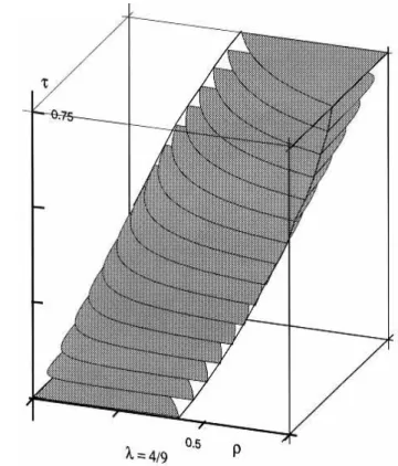
Figure 3 - Constraint cube in ρστ-space. Stability requires that in a medium consisting of isotropic laminae the three parameters are constrained to a cube with one corner at the origin and a side length of 0.75 – compare (6). If all constituents have positive Poisson ratio, the cube has a side length of 0.5. If the ratio θ of squared S- to P-velocities in the constituents lies between θl and θh, the constraint cube has the lower left front corner at (θl, θl, θl,), and the upper right back corner at (θh, θh, θh,).
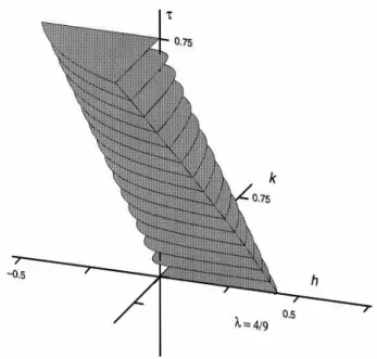
Figure 4 - The constraint parallelepiped in hkτ-space is obtained by ”shearing” the cube in the ρτ- and στ-planes with a shear angle
the volume corresponds to a medium that cannot be modeled by lamination with isotropic constituents.
The first three constraints in Eq. (6) are physical (dictated by stability), while the last is an expression of the Cauchy-Schwartz-Kolmogorov inequality (see Eqs. (8) and (9) below). For this reason (and also in order to avoid the difficult representation of four-dimensional solids) the discussion is restricted to the ρστ-subspace. With the stability constraints of Eq. (6), the constraint volume is a cube with sides 3/4. If the θ are differently (more narrowly) constrained, the constraint cube becomes correspondingly smaller (Fig.3).
If the elastic properties are expressed by the parameters h = ρ – τ, k = σ – τ, τ, the cube changes to a parallelepiped (Fig. 4). The internal geometric relations are, of course, not affected by these two “shearing” operations. 1 0 with , 4 3 0 , 4 3 , 4 3 ≤ λ < < τ < τ − < < τ − τ − < < τ − k h (7)
While every compound medium with isotropic laminae is represented by a point inside the corresponding constraint cube (constraint parallelepiped), not every point inside the cube (parallelepiped) can be so modeled: there are two further constraint surfaces that include a closed volume totally inside the cube. To obtain these, we again use the Cauchy-Schwartz-Kolmogorov inequality:
∑
∑
∑
∑
≤ i i i i i i x w x w w w , (8)where the xi correspond to ”values to be averaged” constrained to a finite interval and the wi correspond to positive ”weights”. Equality pertains only to identical xi. One consequence of this inequality is the observation that the harmonic average is at most equal to the arithmetic average, which was used implicitly to derive c55
≤
c66:(9)
1
,
i i
∑
∑
∑
∑
∑
∑
µ
≤
µ
=
µ
i i i i i i ih
h
h
h
h
h
where the weights hi correspond to the thicknesses of the individual layers, and their sum Σhi = H the
thickness of a “period”.
Berryman (1979) suggested a different use of the inequality: for the wi, one chooses either :
wi = pi(θh-θi), or wi = pi (θi-θl) with pi = H hi (10)
In this formulation, θl is a constant value smaller than any of the θi (i.e., either zero or a lower bound of the actual values), and θh is a constant value higher than any of the θi (i.e., either 3/4, 1/2 or an upper bound of the actual values). As required, all weights are positive. We obtain:
(
)
(
)
(
)
(
)
− − < −∑
∑
∑
∑
∑
∑
∑
i i i i i i i h i i i i h i i h i p p p p p ì 1 ì p ì 1 ì 1 è è ì p ì è è è è i i 2 (11)and a second expression that is obtained by using the second type of weights in Eq. (10). These two inequalities are easily translated to the constraints:
λ(τ-θ1)2<(ρ-θ
1)(σ-θ1),
λ(θh-τ)2<(θ
h-ρ)(θh-σ). (12) With the stability limits θl = 0 and θh = 3/4, one obtains:
λτ2 < ρ σ
λ(3/4-τ)2<(3/4-ρ)(3/4-σ) , (13) which were given in different form already by Backus (1962).
For a formulation in terms of h, k, and τ one can write
θh−ρ = (θh−τ) − (ρ−τ) = (θh−τ)−h = ∆θ+−h,
θh−σ = (θh−τ) − (σ−τ) = (θh−τ)−k = ∆θ+−k,
ρ−θ1 = (ρ−τ) + (τ−θ1) = h+(τ−θ1) = h+∆θ-,
By inserting the corresponding terms from (14) into (12) one obtains:
( ) (
∆θ
+,− 2≤
±
∆θ
+,−)(
±
∆θ
+,−)
,
λ
h
k
(15)where the algebraic signs go with the superscripted signs. By defining ∆θ = ∆θ+, –∆θ–, one can rewrite this as:
λ ∆θ 2 < h – ∆θ k – ∆θ , (15a) where ∆θ can now take positive and negative values (constrained by the expressions in Eq. (6)).
The constraints (6)–(15a) define hypersurfaces in the four-dimensional parameter spaces hkτλ or
ρστλ. The volume enclosed by these hypersurfaces is convex, i.e., if any two points P1 = (ρ1, σ1, τ1, λ1) and P2 = (ρ2, σ2, τ2, λ2) lie inside the constraint volume (satisfy all constraints), then all points P = q P1 + (1 – q) P2 with 0
≤
q≤
1 on the straight segment joining the two points also lie inside the constraint volume.To avoid the problems connected with depicting the four-dimensional constraint volume, we take its intersection with a hyperplane λ = const. Fig. 5 shows the volume defined by (28) for λ = 4/9.
More realistic constraints (instead of the mere requirement that all constituents be stable) restrict the constraint volume further, but in planes τ = const the constraint areas are always bounded by two hyperbolic segments (including, in the planes τ = τmax and τ= τmin,
the asymptotes to the hyperbolae).
The corresponding constraint volume in hkτ-space is obtained by shearing parallel to the planes τ = const (Fig. 6).
Note that the constraint volumes are ”open”, i.e., their surface is excluded. With this specification, any medium with µ = 0 is excluded. It might be tempting to include fluid layers by admitting ”in the limit” vanishing shear stiffness. However, the results thus obtained are misleading: to deal with fluid layers, it is not sufficient to let the shear stiffness of the layers in question vanish. One has also to change the boundary condition from ”welded contact” to ”sliding contact”. Since in the discussion in Part 1 the welded contact is crucial in the definition of the ”fixed” and ”variable” tensor components, such a change cannot be added as an afterthought.
Figure 7 - Top left: contour plot of λ = c55/c66 for a K-medium with two constituents as function of log(µ2/µ1) and δ = (h1 – h2)/ (2(h1 + h2)). Contours at 0.95, 0.9, …. Top right: two-layer representation of a K-medium. Bottom: λ at δ = 0.
Figure 6 - Constraint volume in hkτ-space for λ = 4/9. Note that the K-media are represented by points on the τ-axis.
INVERSION AND UNIQUENESS
The conditions for an inversion of an observed anisotropy with TI symmetry to a periodic sequence of isotropic layers can now be spelled out: if the point representing the medium in one of the parameter spaces lies inside the corresponding constraint volume, such an inversion exists. Further below it will be shown how one can obtain such inversions. Before that, it is important to discuss the meaning of such an inversion. It is obvious that the inversion cannot be unique in the sense that the observed anisotropy must be due to this type of layering. Without further information, there is no way to exclude other causes of anisotropy
Even if any other cause of anisotropy can be excluded, an inversion of stiffness parameters to layer parameters is not necessarily unique. To show this, the simplest (and perhaps most common) case, the inversion of a K-medium to a sequence of layers with the same squared velocity ratio is discussed.
Inversion of a K-medium
Any periodic sequence of isotropic layers with constant θ = (vS/vP)2 is long-wave equivalent to a K-medium with the parameters given in (Part 1, Eq. 24). All terms in Eq. (17) can be expressed through θ = c55/ c33 = (vS⊥/vP⊥)2, <µ> = v
SH||
2, and <1/µ> = 1/v S⊥
2. Thus even complete and accurate observations can yield only these three parameters. The inversion of θ is elementary: each layer must have the same θ as the compound medium. Except for a scale factor, the remaining two can be expressed as their ratio λ = 1/ (<µ> <1/µ>). Any number of layers in the period is possible. To narrow down the possibilities, the number is restricted to two, with shear stiffnesses µ1 and µ2 and relative thicknesses h1 and h2 to be determined.
A symmetric parameterization is:
. h , h and c , e. i. , c / , c 1 δ − 2 1 = δ + 2 1 = = µ µ µ = µ µ = µ 2 2 1 0 2 0 1 , / 2 (16)
This leads to:
(17a)
i.e., there are two equations for the three unkowns µ0, c and δ. After elimination of all stiffnesses, the dimensionless ratio λ = c55/c66 is expressed in terms of the dimensionless ratios c and δ:
2 2 2 1 1 4 1 1 − δ − + = λ c c c c (17b)
One obtains the simplest (and unique) inversion if one assumes two constituents with equal contributions, i.e., δ = 0. The ratio of the shear stiffnesses of the constituents is then:
µ1
µ2δ=0
= c1,2,2 δ=0 =1
λ 2–λ ± 1 – λ . (18) The graphical display of Eq. (18) in Fig.7 shows the low sensitivity of the parameters of a K-medium to deviation from equal contributions of two layers (δ=0):
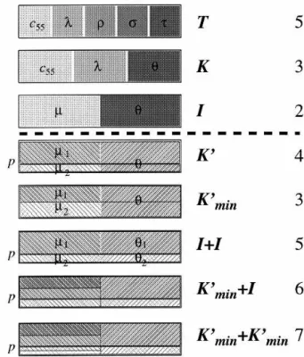
Figure 8 - Top: Three compound media: TI-medium. K-medium,
and isotropic medium. Under the conditions discussed in the text, these media are long-wave equivalent to periodic sequences of isotropic laminae. Below: Basic periods of five simple sequences of isotropic laminae. Two layers with arbitrary thickness but equal
θ (equivalent to a K-medium);Two layers with equal thickness and equal θ (minimum representation of a K-medium); Two arbitrary isotropic layers; An arbitrary isotropic layer combined with two layers with equal thickness and equal θ; Four isotropic layers in two sets of equal thickness and equal θ each. The numbers of parameters are listed on the right.
, − δ + + δ µ = δ + + − δ µ = c c c c c c 2 1 2 1 , 2 1 2 1 0 66 0 55
for a realistic ratio µ2/µ1=2(λ = 0.89), i.e., a ratio of the shearwave velocities of the two constituents of about
2:1, λ remains essentially unchanged for -0.15 < δ <0.15. A reliable determination of the individual contributions requires very accurate determination of
λ.
In the general case (with δ
≠
0) one could either solve for the ratio of the two stiffnesses (with the two contributions assumed or known), or for the two thicknesses. The latter might be more realistic: if the two constituents are, e.g., sand and clay, the individual shear stiffnesses are more or less known, but the relative contribution of these two materials to a compound rock is of great interest. The two (equivalent) solutions are: c1,22 = 1 λ1 – 4 δ2 2– 1 – 4 δ2 λ ± 1 – λ 1 – 4 δ2λ , δ2 = λ 1 + c2 2 – 4 c2 4 λ 1 – c22 .If the shear stiffnesses of the two constituents are known, it is easy to determine the contributions from the observed c66 = <µ> = vSH||2, and c
55 = <1/µ> = vS⊥ 2. In this case, δ can be determined from two independent equations, which should give the same result:
δ = 2c66–µ1 – µ2 µ1 – µ2 ; δ = 2c1 55 – 1 µ1 – 1 µ2 1 µ1 – 1 µ2 = 2µc1µ2 55 –µ2 – µ1 µ2 – µ1 . (20)
Inversion of a general TI medium
Any homogeneous TI medium that satisfies the inequalities (6)–(15) can be inverted to a periodic sequence of isotropic layers. This inversion cannot be unique, since one can always find sequences with three or more layers to match the five constants. However,
it might be of interest to ask for the minimum number of constituents necessary to mach a set of TI constants. The first concern in such an inversion operation is the number of equations versus the number of unknowns. A transversely isotropic medium has five independent stiffnesses. It is not easy to observe all of them, but even with the most elaborate acquisition one has at most five equations. A sequence of two constituents is determined by precisely five parameters (Fig. 8). Thus one might expect that any TI medium can be modeled by two constituents only. Backus (1962) has shown that this is not the case.
To show this, we determine the two-layer sequence that models a medium with given (dimensionless) parameters h, k, τ and λ. For a two-layer sequence, these parameters are related to the layer parameters as:
(
)
(
)(
)
(
)
(
)
(
)
(
)(
)
(
)
(
)
(
)
(
)
(
)
. and , , k , h 2 2 4 4 2 2 4 1 2 2 4 1 2 1 2 1 2 2 1 2 2 2 1 2 1 2 1 2 1 2 1 2 1 2 2 1 2 1 1 2 2 1 2 θ θ δ θ θ τ µ µ δ µ µ µ µ λ µ µ δ µ µ θ θ µ µ δ µ µ δ µ µ θ θ µ µ δ − + + = − − + = − + + − − − = − − + − − − = (21)To make the layer parameters dimensionless too, the two shear stiffnesses are normalized with c66:
(
)
(
)
. 2 2 , 2 2 2 1 2 1 2 * 2 2 1 2 1 1 * 1 µ − µ δ + µ + µ µ = µ µ − µ δ + µ + µ µ = µ (22) Note that: 1 – k h = 2 µ1 + µ2 µ1 + µ2 + 2 δ µ1 – µ2 = µ1* + µ2* and λ k h = –4 µ1µ2 µ1 + µ2 + 2 δ µ1 – µ2 2 = – µ1 *µ 2 * . (23) (19)It follows that the normalized shear stiffnesses are formally the roots of:
h µ*2 – h – k µ* – λk =0, i.e., µ1, 2* = 12 1 – kh ± 1 – kh2 + 4 λkh = 1 2 1 – kh ± 1 – kh–2λ 2 + 4 λ 1 – λ . (24)
This solution is meaningful if both normalized shear stiffnesses are real and positive. This is the case if 0
≤
λ ≤ 1 (which is guaranteed) and if k/h < 0. TI media satisfying the constraints (6) – (15) thus are long-wave equivalent to a layer sequence with two constituents if and only if h and k have different algebraic sign. Thus media with h k > 0 cannot be modeled by only two constituents.If the two roots of Eq. (24) are positive and real, the medium can be modeled by two constituents, and the remaining parameters are easily determined:
(
)
(
)
(
)
(
)
(
(
)
)
(
)
(
)
(
)
, 1 1 1 θ , -1 -1 -1 θ , λ 1 4 λ λ 2 1 2 1 2 2 2 2 , 2 µ µ 2 δ µ µ 1 2 2 * 1 * 1 * 1 2 * 2 * 2 * 2 1 2 2 1 2 1 66 * 2 * 1 * 2 * 1 * 2 * 1 * 2 * 1 2 1 2 1 66 − µ − = − µ − − µ = µ + = µ − µ = − + − − + = = µ − µ µ + µ − = µ − µ µ + µ − = δ − + + = ⇒ µ − µ δ + µ + µ = k τ k τ k τ k τ h k h k c c ( 25) This solution is unique: if a transversely isotropic medium is long-wave equivalent to a periodic sequence with two constituents only, it can be modeled in one and only one way. It can, of course, be modeled in many different ways with more than two constituents. If h and k have the same sign, the product of the two roots of Eq. (23) is negative, i.e., one of the roots must be negative and thus cannot be accepted as a normalized shear stiffness. Backus (1962) showed that such a medium can be modeled by two K-media (thelast model in Fig. 8). If the K-media are chosen as minimum-representations (δ = 0), this requires seven parameters. The inversion thus leaves two parameters free for a two-dimensional manifold of equivalent solutions. Actually, Backus (1962) stated in the text that this was a model with four isotropic constituents, and asserted without proof that by an intricate argument the model could be reduced to three isotropic constituents. An arbitrary combination of three isotropic layers would have eight parameters. Helbig (1981) showed that a medium with sig(h) = sig(k) can be modeled by a K-medium and an isotropic medium. This combination of three isotropic constituents has – if the K-medium is chosen with equal thickness for the two constituents – six parameters, thus the inversion is still a one-parametric manifold. Note that the K-medium can only be determined within the limits shown in Eq.(19) and in Fig. 7, so that the inversion is a two-parametric manifold.
The proof is lengthy (for details see Helbig (1981, 1994)). For this reasons, only the main lines are given: a model with three constituents is described by:
h1+ h2+h3= 1, h1µ1* +h2µ2* +h3µ3* = 1 , h1θ1µ1* +h1θ2µ2* +h3θ3µ3* = σ , h1θ1 +h2θ2 +h3θ3 = τ , h1θ1 µ1* +h2θ2 µ2* +h3θ3 µ3* = ρ , and h1 µ1* + h2 µ2* + h3 µ3* = 1 λ , (26)
where the shear stiffnesses have been normalized by c66. The θi and µi satisfy the stability constraints for
isotropic media, and the ρ, σ, τ, and λ the constraints for a TI medium that is long-wave equivalent to a periodic sequence of layers ((6) – (15)).
Assume that the normalized shear stiffnesses 0 < µ1* < µ2* < µ3* are known. The six equations (26) split into two groups: three can be used to determine the three hi, the remaining three to determine the three θi. The formal solutions are:
In view of the ranking of the normalized shear stiffnesses, the denominators of the expressions for h1 and h3 are positive, that for h2 negative. Since all h and
θ must be positive, the remaining numerators and denominators of all six expression must have the same signs as the first three denominators: the numerators of the expressions for h2 and θ2 must be negative, the other four numerators positive. Further three inequalities can be derived from the conditions 0 < {ρ, σ, τ} < 3/4. The nine inequalities result in upper bounds for µ1* and lower bounds for µ3*, and some ”interaction bounds” on one of the two if the other is given a value that satisfies the ”non-interaction bounds”. In any case, the ”outer” two shear stiffnesses can always be chosen in such a way that the bounds are satisfied. For the ”central” shear stiffness there is always an interval in the middle of the range such that all inequalities are satisfied: h < 0 , k < 0 h > 0 , k > 0 λ ρτ < µ2* < σ τ λ 34 – τ 34 – ρ < µ2 * < 34 – σ 34 – τ (28)
Instead of setting up all inequalities and choosing the normalized shear stiffnesses correspondingly, one can make use of the fact that the positive root of (24) lies in the interval for the central shear stiffness. This is shown by writing (24) as a function:
F(µ*) = h µ*2 -(h-k)µ*-λk. (29) Since the function is continuous, there is precisely one root in the intervals of Eq. (28) if the function has different algebraic signs at the ends of the interval:
h<0,k <0 h >0 ,k >0 F λ τ ρ = – h ρλ2 ρ σ – λ τ 2 F λ 34 – τ 34 – ρ = – h λ 34 – ρ 34 – σ – λ 34 – τ 2 3 4 – ρ 2 F σ τ = k τλ2 ρ σ – λ τ 2 F 34 – σ 3 4 – τ = k λ 34 – ρ 34 – σ – λ 34 – τ2 3 4 – τ 2 . ; (30)
Thus it is always possible to choose three shear stiffnesses in such a way that all inequalities are satisfied. The remaining parameters are then determined with Eq. (27).
Next it is shown that this choice of the central shear stiffness forces the other two constituents to have the same θ. By subtracting the expressions for θ1 and θ3 in Eq. (27), one obtains:
h1 = 1 + µ2 µ3 λ – µ2 + µ3 µ1 + µ2µµ3 1 – µ2 + µ3 , and θ1 = σ+ ρ µ2 µ3 λ – τ µ2 + µ3 1 + µ2 µ3 λ – µ2 + µ3 , h2 = 1 + µ1 µ3 λ – µ1 + µ3 µ2 + µ1µµ3 2 – µ1 + µ3 , θ2 = σ + ρ µ1 µ3 λ – τ µ1 + µ3 1 + µ1 µ3 λ – µ1 + µ3 , h3 = 1 + µ1 µ2 λ – µ1 + µ2 µ3 + µ1µµ2 3 – µ1 + µ2 , θ3 = σ+ ρ µ1 µ2 λ – τ µ1 + µ2 1 + µ1 µ2 λ – µ1 + µ2 . (27)
Formally, θ1 and θ3 follow from (27) as θ1 = k + τ 1 – µ2 * + µ 3 * h + τ λ µ2 * – τ 1 – µ2 * + µ3 * µ2 * λ – 1 , θ3 = k + τ 1 – µ2 * + µ 1 * h + τ λ µ2 * – τ 1 – µ2 * + µ1 * µ2 * λ – 1 . (32)
These two expressions must be equal and independent of the – as yet undetermined – µ1*, µ
3*, thus the coefficients of these two stiffnesses can be set to zero to yield:
θ1, 3 = k +τ 1 – µ2 * 1 – µ2* =τ + k 1 – µ2* . (33) To choose the outer shear stiffnesses we make the arbitrary choice h1 = h3. With that we obtain:
c66(K) = c66 µ1 * + µ3* 2 , c55 (K) = c 66 2µ1 * µ3* µ1* + µ3* . (34) The condition h1 = h3 yields with (27) another quadric in µ2*:
(35)
µ2* is a root of both (24) and (35), thus the coefficients must be proportional. This leads to:
(
)
, 1 1 µ µ , 1 2 µ µ * 3 * * 3 * 1 1 h a k a k a + + λ = + = + (36)with an as yet undetermined a. Once three shear stiffnesses have been chosen, equations (27) can be used to determine the remaining parameters. For instance, one obtains for θ2:
θ2 = τ + k 1 – µ1 * + µ 3 * 2 . (37)
Practical inversion
In the previous section it was shown that it is always possible to model any sequence of layers with at most six free parameters. This is important as a lower bound, but for the practical inversion of minor importance. One often knows some parameters of some constituents, which may not be those suggested by the solution in Eqs. (27)–(37). In such a case the problem is to determine the remaining constituents. Since the three normalized shear stiffnesses are constrained to genuine intervals – i.e., each can assume an infinite number of values – the set of all possible solutions is a three-parametric manifold. It is thus possible to choose three parameters. The choice is not entirely arbitrary: for instance, if h and k have the same algebraic sign, µ2* must lie in the corresponding intervals Eq. (27), and the outer two shear stiffnesses must lie outside the respective bounds:
h >0, k >0 µ1* < λρτ ; στ < µ3* h <0, k <0 µ1* < λ 34 – τ ; 34 – ρ 34 – σ 34 – τ < µ3 * . (38) θ1 – θ3 = µ3 * – µ 1 * λ = 0 h µ2 *2 – h – k µ2* – k λ 1 + µ2* µ3 * λ – µ2 * + µ 3 * 1 + µ2 * µ1* λ – µ2 * + µ 1 * . 1 x x x x (31) µ1* + µ3* 2 µ1* µ3* – 1 λ * 2 µ2*2 + µ µ1 * + µ3 * 2 λ – µ1 * + µ3 * 2 µ1 * µ3 * + 1 – µ1 * + µ3 * λ = 0. + +
If one of the outer stiffnesses is chosen, the other has to satisfy, respectively,
Any choice of shear stiffnesses that satisfies Eqs. (28) and (38, 39) leads in Eq. (27) to meaningful θi and hi.
The conditions for compound media with three constituents and h k < 0 have not been investigated.
CONCLUSIONS
Any sequence of isotropic layers leads to long-wave transverse isotropy of the compound medium. If the sequence is periodic, the compound medium is (long-wave) homogeneous. The requirement that the constituents are stable leads to inequalities between the parameters of the compound medium. As a consequence, only TI media for which these inequalities are satisfied can be ”modeled” by layer sequences.
Observed anisotropy can be used to determine its causes, though additional information is required to restrict the type of causes. If the anisotropy is due to layering, if the elastic tensor is completely determined, and if all inequalities between the parameters are satisfied, layer sequences to produce the transverse isotropy can be found. Under certain conditions, a unique decomposition into two constituents is possible, but a decomposition into three constituents is always possible. Since three constituents are determined by eight parameters and the TI compound medium by five, the
set of all possible solution is a three-parametric manifold, i.e., three parameters can be chosen or must be determined independently.
The complete determination of the elastic parameters from surface observation alone is not generally possible. This is illustrated by the K-medium, that is long-wave equivalent to a sequence of constituents with a common ratio of S- to P-velocities, which is a realistic assumption. Such media can be strongly anisotropic, but P-wave observation over an aperture of about 30° would show no deviation from isotropy (Part 1, Fig. 4).
The inversion of TI elastic constants to those of the constituents for lithological purposes – e.g., to get information on the inner structure of a reservoir – thus can be useful only in conjunction with other methods. As a stand-alone method it is bound to disappoint.
REFERENCES
AYRES, F. JR– 1962–Matrices. Schaum’s Outline Series, McGraw–Hill.
BACKUS, G.E.–1962–Longwave elastic anisotropy produced by horizontal layering. Journal of Geophysical Research, 67: 4427–4440.
BERRYMAN, J.G.–1979–Long wave elastic anisotropy in transversely isotropic media. Geophysics, 44: 896–917. HELBIG, K.–1958–Elastische Wellen in anisotropen Medien. Gerlands Beiträge zur Geophysik, 67 (177–211);256–288. HELBIG, K.–1979–Discussion on ”The reflection, refraction and diffraction of waves in media with elliptical velocity dependence” (F.K. Levin). Geophysics, 44: 987–990. HELBIG, K.–1981–Systematic classification of layer–
induced transverse isotropy. Geophysical Prospecting, 29: 550–577.
HELBIG, K–1994–Foundations of Anisotropy for Exploration Seismics. Handbook of Geophysical Exploration Vol. 22 sect. I, Seismic Exploration (K. Helbig & S. Treitel, Ed.), Pergamon.
HELBIG, K–1998–Layer-induced anisotropy – forward relations between constituent parameters and compound parameters. Brazilian Journal of Geophysics, 16(2–3): 103-114.
POSTMA, G.W.–1955–Wave propagation in a stratified medium. Geophysics, 20: 780–806.
RUDZKI, M.P.–1911–Parametrische Darstellung der elastischen Welle in anisotropen Medien. Bulletin International de’l Academie de Sciences et de Lettres de Cracovie, Classe de Sciences mathématiques et naturelles, Serie A: 503–536. h > 0, k > 0 µ1* < λ τµ3* – σ ρ λ µ3 * – τ σ – τµ1* τ– ρ λ µ1 * < µ3* h <0, k < 0 µ1* < λ 3 4 – τ µ3* – 34 – σ 3 4 – ρ λ µ3 * – 3 4 – τ 34 – σ
–
34 – τ µ 1 * 3 4 – τ – 34 – ρ λ µ1 * < µ3* . ; ; (39) Klaus HelbigSee Brazilian Journal of Geophysics, 18(2-3) p. 114