Chromatic filters for color vision deficiencies

Universidade do Minho

Escola de Ciências

Ruben Carpinteiro Pastilha

junho de 2018

Chromatic filters for color vision deficiencies

Ruben Carpinteiro Pastilha

Chromatic filter

s for color vision deficiencies

Universidade do Minho

Escola de Ciências

Ruben Carpinteiro Pastilha

junho de 2018

Chromatic filters for color vision deficiencies

Trabalho realizado sob orientação do

Professor Doutor Sérgio Miguel Cardoso Nascimento

e do

Professor Doutor João Manuel Maciel Linhares

Dissertação de Mestrado

Declaração Nome: Ruben Carpinteiro Pastilha

Endereço eletrónico: rubenpastilha@gmail.com

Telefone: 917621898

Número do Cartão de Cidadão: 14366568 5 ZY8

Título da Dissertação de Mestrado:

Chromatic filters for color vision deficiencies

Orientadores:

Professor Doutor Sérgio Miguel Cardoso Nascimento Professor Doutor João Manuel Maciel Linhares

Ano de conclusão: 2018

Designação do Mestrado: Mestrado em Optometria Avançada

DE ACORDO COM A LEGISLAÇÃO EM VIGOR, NÃO É PERMITIDA A REPRODUÇÃO DE QUALQUER PARTE DESTA DISSERTAÇÃO.

Universidade do Minho, ___/___/______

iii

Acknowledgments

I would like to express my outmost gratitude to my advisors, Professor J Sérgio Miguel Cardoso Nascimento and Professor João Manuel Maciel Linhares, for all their support, guidance, knowledge and companionship.

I would like to thank my parents, brothers, girlfriend, and friends for all their help and support.

I would also like to thank my friends and colleagues from the Color Science Lab and the dermatology service of the Coimbra Hospital and Universitary Centre for all their collaboration and contribution to this work.

And I would like to thank all color vision defectives and control participants, for their kindness and availability, and all those who somehow contributed to the completion of this work.

v

Abstract

About 10% of the population have some form of color vision deficiency. One of the most sever deficiencies is dichromacy. Dichromacy impairs color vision and impoverishes the discrimination of surface colors in natural scenes. Computational estimates based on hyperspectral imaging data from natural scenes suggest that dichromats can discriminate only about 7% of the number of colors discriminated by normal observers on natural scenes. These estimates, however, assume that the colors are equally frequent. Yet, pairs of color confused by dichromats may be rare and thus have small impact on the overall perceived chromatic diversity. By using an experimental setup that allows visual comparation between different spectra selected form hyperspectral images of natural scenes, it was estimated that the number of pairs that dichromats could discriminate was almost 70% of those discriminated by normal observers, a fraction much higher than anticipated from estimates of the number of discernible colors on natural scenes. Therefore, it may be rare for a dichromat to encounter two objects of different colors that he confounds. Thus, chromatic filters for color vision deficiencies intended to improve all colors in general may constitute low practical value. On this work it is proposed a method to compute filters specialized for a specific color-detection task, by taking into account the user’s color vision type, the local illuminant, and the reflectance spectra of the objects intended to be distinguished during that task. This method was applied on a case of a medical practitioner with protanopia to idealize a filter to improve detection of erythema on the skin of its patients. The filter improved the mean color difference between erythema and normal skin by 44%.

vii

Resumo

Cerca de 10% da população possui alguma forma de deficiência de visão de cor. Uma das deficiências mais severas é a dicromacia. Dicromacia prejudica a visão das cores e empobrece a discriminação de superficies coloridas em cenas naturais. Estimativas computacionais baseadas em dados de imagens hiperespectrais de cenas naturais sugerem que dicromatas só pode discriminar cerca de 7% do número de cores discriminadas por observadores normais em cenas naturais. Estas estimativas, no entanto, assumem que todas as cores são igualmente frequentes. Contudo, pares de cores confundidos por dichromats podem ser raros e, portanto, têm pequeno impacto na diversidade cromática global percebida. Ao usar uma montagem experimental que permite comparação visual entre espectros diferentes selecionados a partir de imagens hiperespectrais de cenas naturais, estimou-se que o número de pares que dicromatas poderiam discriminar era quase 70% dos discriminados por observadores normais, uma fração muito maior do que o antecipado a partir de estimativas do número de cores percebidas em cenas naturais. Portanto, pode ser raro para um dicromat para encontrar dois objetos cujas cores ele confunda. Assim, filtros cromático para deficiências de visão das cores pretendidos para melhorar todas as cores em geral podem constituir baixo valor prático. Neste trabalho é proposto um método para calcular filtros especializados para uma tarefa específica de detecção de cor, tendo em conta o tipo de visão de cor do utilizador, o iluminante local, e os espectros de reflectancia dos objetos pretendidos a serem distinguidos durante essa tarefa. Este método foi aplicado em um caso de um médico com Protanopia para idealizar um filtro para melhorar a detecção de eritema na pele de seus pacientes. O filtro melhorou a diferença média de cor entre o eritema e a pele normal por 44%.

ix

Index

INTRODUCTION AND RESEARCH RATIONALE ... 19

CHAPTER 1. LITERATURE REVIEW ... 23

1.1. The visual process ... 24

1.1.1. The retina ... 24

1.1.2. In the lateral geniculate nucleus ... 25

1.1.3. In the cortex ... 26

1.2. Color Vision ... 27

1.1.4. The evolution of color vision... 27

1.1.5. Color perception ... 28

1.1.6. Color vision deficiencies ... 28

1.1.7. Solutions for color vision deficiencies ... 32

1.3. Colorimetry... 33

1.1.8. Tristimulus XYZ ... 34

1.1.9. CIELAB ... 35

1.1.10. Color ordered systems ... 36

CHAPTER 2. COMPARISON BETWEEN NATURAL COLORS OF THE MINHO REGION AND ARTIFICIAL COLORS OF COLOR ORDERED SYSTEMS – MUNSELL AND NCS ... 37

x

2.1. Introduction ... 38

2.2. Methods ... 39

2.3. Results ... 42

2.4. Discussion ... 47

CHAPTER 3. THE COLORS OF NATURAL SCENES BENEFIT DICHROMATS ... 49

3.1. Introduction ... 50 3.2. Methods ... 51 3.2.1. Experimental setup ... 51 3.2.2. Stimuli ... 52 3.2.3. Procedure ... 54 3.2.4. Observers ... 55 3.3. Results ... 56 3.4. Discussion ... 57

CHAPTER 4. DATA BASE OF SPECTRAL DATA FROM NORMAL AND ABNORMAL SKIN OF HOSPITAL PATIENTS. ... 59 4.1. Introduction ... 60 4.2. Methods ... 60 4.2.1. Participants ... 61 4.2.2. Skin measuring ... 61 4.3. Results ... 63 4.4. Discussion ... 66

CHAPTER 5. COMPUTATION OF A COLORED FILTER TO IMPROVE ERYTHEMA DETECTION ON THE SKIN OF PATIENTS FOR A MEDICAL PRACTITIONER WITH PROTANOPIA – A CASE REPORT. ... 67 5.1. Introduction ... 68 5.2. Methods ... 69 5.2.1. Appointed illuminant ... 69 5.2.2. Filter computation ... 70 5.3. Results ... 72

xi

5.3.1. Filter optimization ... 72

5.3.2. Filter assessment ... 73

5.4. Discussion ... 76

CHAPTER 6. CONCLUSION AND FUTURE WORK ... 79

6.1. Main conclusions ... 80

6.2. Future work ... 80

REFERENCES ... 81

APPENDICES ... 97

Appendix I. Model of informed consent for the experiment of Chapter 3 ... 99

Appendix II. Research protocol submitted to the SECVS ethics committee of the University of Minho. . 101

Appendix III. Copy of the approval given by the SECVS ethics committee of the University of Minho. .. 117

Appendix IV. Acquisition record sheet ... 119

xii

Abbreviations and acronyms

CHUC: Centro Hospitalar e Universitário de Coimbra (Coimbra Hospital and Universitary Centre) CIE: Commission Internationale de l’Eclairage (International Commission on Illumination) CVD: Color vision deficiency

HRR: Hardy-Rand-Rittler test

L: relative to the cone type sensitive to long visible wavelengths. LGN: Lateral Geniculate Nucleus

M: relative to the cone type sensitive to middle visible wavelengths. MCS: Munsell Color System

MBC: Munsell Book of Color NCS: Natural Color System

pRGC: Photosensitive Retinal Ganglion Cells

S: relative to the cone type sensitive to short visible wavelengths. SC: Superior Colliculus

SD: Standard Deviation

SECVS: Subcomissão de ética para as ciências da vida e da saúde (Subcommission of Ethics for Life and Health Sciences)

xiii

Index of figures

Figure 1.1. Schematic representation of a vertical section of the eye highlighting the retinal layers (adapted from [20]). ... 24 Figure 1.2. Relative spectral sensitivity of the cone types, In linear units of energy and assuming a visual field of 2º (adapted from [29]). The S, M and L cones are represented respectively by the blue, green and red lines. ... 25 Figure 1.3. Schematic representation of the optic pathway (viewed from above), showing how the optical fibers are organized in the optical chiasm (adapted from [31]). ... 26 Figure 1.4. Orientations of the confusion lines of the three types of dichromats, protanope (left panel), deuteranope (middle panel), and tritanope (right panel), plotted on the Judd revised chromaticity diagram (adapted from [69]). ... 29 Figure 1.5. Limits of the object-color solid in CIELAB color space under illuminant D65 for normal observers and color vision defectives (adapted from [12]). ... 30 Figure 1.6. Color matching functions 𝑥(𝜆), 𝑦𝜆, and 𝑧(𝜆) of the CIE 1931 standard colorimetric observer (solid lines) and 𝑥10(𝜆), 𝑦10𝜆, and 𝑧10(𝜆) of the CIE 1964 standard colorimetric observer (dashed lines) (adapted from [8,11]. ... 34 Figure 1.7. Schematic representation of the coordinate system that make the tree-dimensional CIE 1976 (L*a*b*) color space (adapted form [115]). ... 35 Figure 2.1. Representation of the natural colors obtained from spectral imaging (a), Munsell Color System (b) and Natural Color System (c) in CIELAB color space. Colors were computed assuming D65 illuminant. For illustration purposes only a fourth of the data points of (a) are represented.41 Figure 2.2. Color distributions of the three data sets. Colored solid lines represent mean frequency of colors across 60 illuminants and the corresponding range for the illuminant set (colored shaded area). ... 42 Figure 2.3. Results of the convex hull and point analysis. (a) The CIELAB diagram represents for the CIE standard illuminant D65 the convex hulls of the natural colors (grey solid line), MCS (blue solid line), and NCS (red solid line). (b) Fraction of the volume and areas of natural colors occupied by the color systems. (c) Fraction of the natural colors inside each color system. (b) and (c) represent mean data across the illuminants set. ... 43

xiv

Figure 2.4. Results of the color difference analysis. (a) and (c) Represent the relative frequency and cumulative frequency, respectively, of color differences expressed in CIELAB between each natural color from the set of natural scenes (NS) and the corresponding one in the MCS or NCS. (b) and (d) Represent similar data but for the subset (NS’) of the natural colors which includes only data points within the volume of each color system. Data represent mean across illuminants for MCS (blue solid line) and NCS (red solid line) and corresponding range across illuminants for MCS (blue shaded area) and NCS (red shaded area). ... 44 Figure 2.5. Variations of ∆E color differences between the COS and natural colors across the color space. Voronoi diagrams map ∆E values for a*b*, L*a*, and L*b* between each natural color and the corresponding color of MCS (a) and NCS (b). Data corresponds to the colors of Figure 2.1 assuming D65 illuminant. ... 46 Figure 3.1. Front view of the test setup (A), close view of the test scene (B), and the radiance spectrum of the discharge lamp (OSRAM HQI 150W RX7s) reflected by the white Styrofoam mask that served as the adapting illuminant for the experiment (C). The white Styrofoam mask illuminated by the adapting illuminant provided an adapting field. A rectangular aperture on this mask allowed the scene to be seen by the observer. ... 51 Figure 3.2. Images of the four natural scenes tested. Scenes A and B are from rural environments. Scenes C and D are from urban environments. The scenes represented in A and B are from the Minho region, C is from Braga and D is from Porto, all in Portugal. They belong to an existing database [130,131]. The colors of the scenes were simulated as illuminated by the adapting illuminant. In each trial of the experiment two pixels were selected randomly and their radiance spectra were used to illuminate successively the objects inside the booth. Each scene was tested in different experimental sessions. ... 53 Figure 3.3. Color volume of each natural scene represented in Figure 3.2. The illumination was the adapting illuminant with a CCT of 5200 K and the colors are represented in the CIELAB color space for the CIE 1964 standard observer. ... 54 Figure 3.4. Stimuli sequence of each trial. The experiment was a 1AFC single alternative same-different test. The adapting illuminant was kept on for the first 1.5 s of the trial. The two test spectra and the three dark ISI lasted 0.5 s each. The adapting illuminant was the same in all trials but spectrum 1 and spectrum 2 varied between trials. ... 55

xv

Figure 3.5. Results from the experiment for normal observers (N) and dichromats, protanopes (P) and deuteranopes (D). (A) Average pairs of colors identified as different. (B) Average discrimination index d’ computed for an 1AFC, same-different task by the differencing mode [150]. (C) Average pairs of colors identified as different derived by the discrimination index d’ assuming that all observers have the same criterion. Data based on 2640 trials for each observer. Error bars represent standard error across observers. ... 56 Figure 4.1. Age distribution of the participants recruit at the hospital. ... 61 Figure 4.2. Contact spectrophotometer (CM-2600D, Konica Minolta, Japan) used for measuring dermatological patients. For biological protection it was repacked with a new plastic protector for every new patient. The transparent plastic covered the measure sensor ate the bottom of the instrument and therefore its calibration had to be made having g the plastic in account. ... 62 Figure 4.3. The 7 body locations of the normal skin measures (forehead, right cheek, left cheek, back of right hand, back of left hand, right inner forearm, and left inner forearm). ... 63 Figure 4.4. Mean reflectance spectra of the normal skin on forehead, cheeks, back of hands, and inner forearms. The data of the 83 Caucasian are presented on (a) and (b) shows the same data for the only African participant. ... 64 Figure 4.5. Pictures and mean reflectance spectra of examples of abnormal skin cases. ... 65 Figure 5.1. Mean radiance spectrum of the work place illuminant indicated by the protanope medical practitioner to be used in the filter computations. ... 69 Figure 5.2. Representation in projections of the CIELAB color space planes of the colors perceived by a protanope, for the data sets of normal skin (a) and erythema (b). Similar data is also shown for the CIE 1931 standard observer in (c) and (d), respectively. It is assumed the appointed illuminant. ... 71 Figure 5.3. Filter transmittance spectrum optimized for erythema detection, for protanope (red line) and for normal CIE 1931 standard observer (blue line). ... 72 Figure 5.4. Spectral effect of the computed filters on the radiance spectra of normal skin (blue lines) and erythema (red lines). Comparison between the radiance spectra of skin seen through the filters (solid lines) and the original spectra (dashed lines), for the protanope filter (a) and the filter computed for the CIE 1931 standard observer (b). ... 73

xvi

Figure 5.5. Chromatic effect of the computed filters. Representation of skin colors (normal skin and erythema) by its 2-D projections on planes of the CIELAB color space, as seen by the protanope observer, without filter (a) and with filter (b). Similar data is also shown for the CIE 1931 standard observer in (c) and (d), respectively. It is assumed the illuminant of Figure 5.1. ... 74 Figure 5.6. Comparison of color difference results for skin observation without filter (dashed lines) and with filter (solid lines). (a) and (b) Represent the relative frequency and cumulative frequency, respectively, of the color differences expressed in CIELAB between the data sets of normal skin and erythema when viewed by a protanope. (c) and (d) Represent similar data but assuming the normal CIE 1931 standard observer. ... 75

xvii

Index of tables

Table 1.1. Incidence of hereditary CVD (adapted from [9,69])... 31 Table 4.1. Data base of Caucasian skin samples organized by type of clinical sign. ... 64

19

Introduction and research rationale

Normal human color vision is trichromatic, based on three type of cone photoreceptors with photopigments absorbing light in the short-, medium- and long-wavelength regions of the visible spectrum [1]. It evolved from the Old World primates who developed trichromatic vision about 40 million years ago [2], probably as an adaptation for foraging [3,4]. It allows discrimination of several million surface colors [5,6]. With the possible exception of tetrachromatic women [7] the genetic anomalies underlying color deficiencies imply limitations in color discrimination either because photopigments are spectrally closer, like in anomalous trichromats, or missing, like in dichromats or monochromats [8].

Dichromacy is most frequent in the red-green range of the spectrum because the photopigments are X-linked and individuals lack either the long-wavelength-sensitive (L) cones (protanopes) or the middle-wavelength-sensitive (M) cones (deuteranopes). It affects a small number of females, about 0.02%, but a larger number of males, about 2% [9]. Dichromats confound colors that are discriminated by normal trichromats. Estimates based on Brettel’s dichromatic perceptual model [10] and on how much the object color volume [11] is compressed in dichromacy predict that dichromats see less than 1% percent of the object colors that normal trichromats can see [12]. These estimates, however, assume that the all colors are possible and equally frequent. Yet, pairs of colors confused by dichromats may be rare and thus have small impact on overall perceived chromatic diversity.

Chromatic filters have the potential to improve the chromatic diversity [13–18] and may be useful as a compensation for dichromacy.

To explore some of these aspects, the present dissertation was developed covering the following main issues:

1) Performance of Dichromats’ dealing with the colors of the possible to encounter in rural and urban environments.

2) Computation of chromatic filters specialized to improve a dichromat’s color discrimination on a specific color-related task.

20

The common line of reasoning linking the whole work is expressed in the following summary of showing the organization of chapters and how they relate to each other:

Chapter 1. Literature Review

The Chapter 1 is a literature review that address the fundamentals of the visual process, color vision and colorimetry that are the intellectual foundation for the following chapters.

Chapter 2. Comparison between natural colors of the Minho region and artificial colors of color ordered systems – Munsell and NCS

This chapter corresponds to a study, done recently by the candidate, that compares natural colors of the world to the sets of artificial color samples of two color ordered systems. This study is not directly related to color vision deficiencies, but provides as secondary result a statistics analysis on the colors of an existing hyperspectral images data base that was used on Chapter 3 and therefore, it was thought to be a useful inclusion on the dissertation.

Chapter 3. The colors of natural scenes benefit dichromats

This study estimated, empirically, how much dichromats are impaired in discriminating surface colors drawn from natural scenes. The stimulus for the experiment was a scene made of real three-dimensional objects painted with matte white paint and illuminated by a spectrally tunable light source. In each trial the observers saw the scene illuminated by two spectra in two successive time intervals and had to indicate whether the colors perceived in the two intervals were the same or different. The spectra were drawn randomly from hyperspectral data of natural scenes and therefore represented natural spectral statistics. Four normal trichromats and four dichromats carried out the experiment. It was found that the number of pairs that could be discriminated by dichromats was almost 70% of those discriminated by normal trichromats, a fraction much higher than anticipated from estimates of discernible colors.

21

Chapter 4. Data base of spectral data from normal and abnormal skin of hospital patients.

The purpose of this work was to construct a data base of spectral reflectance of normal and abnormal skin of hospital patients to be implemented on the computations at Chapter 5 of a colored filter for a medical practitioner with protanopia. Several skin disorders were measured along with normal skin samples. But the data set of erythema was the only data set of abnormal skin with satisfactory sample size to use on Chapter 5.

Chapter 5. Computation of a colored filter to improve erythema detection on the skin of patients for a medical practitioner with protanopia – a case report.

The findings of Chapter 3 suggest that dichromats can distinguishing colors of general environments almost as well as normal trichromats. Therefore, they may not need CVD filters to discriminate all colors in general, and could benefit more from filters optimized for specific objects and situations. On Chapter 5 it is proposed a method to compute CVD filters specialized for the user, by considering the dichromacy type, work place illumination, and the spectra of the objects desired to detect. This method was applied to idealize a filter to help a medical practitioner with protanopia to detect skin abnormalities like erythema. It was used the erythema data and normal skin data acquired on Chapter 4

Chapter 6. Conclusion and future work

This final chapter summarizes the main conclusions of the previous chapters highlighting the main outcomes of the work and indications for future work in the research lines addressed.

23

Chapter 1. Literature Review

24

1.1. The visual process

The visual system consists of a set of organs that cooperate with each other to produce an interpretation of the environment using a specific portion of the electromagnetic spectrum. The visual process begins in the eye whose anatomy and physiology allow the capture of light. Figure 1.1 shows the optics of the eye focusing the light rays and projecting an optical image onto the retina. Light travels through the retinal layers and reach the photoreceptors layer hitting photosensitive pigments that trigger the process of light transduction converting light into electric energy, thus coding the light signal [19,20]. The nerve electrical signal is then sent throughout the optic nerve way for visual processing.

Figure 1.1. Schematic representation of a vertical section of the eye highlighting the retinal layers (adapted from [20]).

1.1.1.

The retina

The human retina has an average of about 92 millions of rods, mostly distributed in the peripheral retina and absent in the foveola [21]. The average number of cones in the retina is approximately 4.6 millions of cones and its maximum density is found on the foveola with an average value of 199 000 cones per mm2 [21]. It is possible to distinguish three types of cones (S,

M and L) that contain pigments with different sensitivities to the wavelengths of the visible spectrum. The relative sensitivity spectra of each cone type are represented in Figure 1.2.

The electric signal generated at the cones and rods is transmitted as a nervous impulse across the remaining nerve cells of the retina: bipolar, horizontal, amacrine, and the ganglion cells whose fibers group together to form the optic nerve. The retinal signals transported by the optic nerve carries with it a preliminary level of organization and modulation indicating that the processing of the visual signal begins in the retina [20].

25

The cones and rods are not the only photosensitive cells in the mammalian retina. Some ganglion cells were identified as having their own photosensitive molecule, the melanopsin [22]. These photosensitive retinal ganglion cells (pRGC) were traditionally associated with physiological responses to light, like regulation of circadian rhythms and pupilar response [23]. But recently has been suggested that pRGC may also contribute to visual perception, specifically in the perception of brightness [24,25] and color [26–28].

Figure 1.2. Relative spectral sensitivity of the cone types, In linear units of energy and assuming a visual field of 2º (adapted from [29]). The S, M and L cones are represented respectively by the blue, green and red lines.

1.1.2.

In the lateral geniculate nucleus

Figure 1.3 shows how the optic nerve of each eye branches in the optic chiasm sending the ganglion fibers of the nasal retina to the contralateral hemisphere. Thus, information of the left visual field will be processed by the right side of the brain and vice versa. About 90% of these fibers connect to the lateral geniculate nucleus (LGN) located at the thalamus [30]. The remaining fibers connect to the superior colliculus (SC) in the midbrain and assumes a role on the control of eye movements and other visual behaviors [30].

0 1 390 445 500 555 610 665 720 rel at ive sen sitivi ty wavelength (nm) S(λ) M(λ) L(λ)

26

Figure 1.3. Schematic representation of the optic pathway (viewed from above), showing how the optical fibers are organized in the optical chiasm (adapted from [31]).

The LGN presents a laminated structure of 6 main layers. The main function of the LGN is to organize and regulate the flow of neural information coming from the retina before being sent to the visual cortex [32,33]. The retinal signals that reach the LGN are organized in three parallel neurological pathways: magno-, parvo-, and koniocellular pathways. These pathways correspond to distinct sets of LGN cells that connect different types of ganglion cells to specific areas of the primary visual cortex. The neurons of each LGN layer are distributed in a spatial organization concordant with the spatial organization of the correspondent receptive fields in the retina [32,33].

The two ventral layers of the LGN correspond to the magnocellular pathway which is believed to be involved in the perception of movement and contrast sensitivity [34,35]. The four dorsal layers belong to the parvocellular pathway which presents smaller receptive field cells involved in the visual acuity process and possibly also in the color vision [34–37]. In between these 6 layers lays the cells of the Koniocellular pathway. These cells receive the signal of the S cones and therefore contribute to color vision [36,38].

1.1.3.

In the cortex

The information from the LGN is transmitted to the visual areas of the cortex where the most complex visual processing occurs and the perceived image is generated. The primary visual cortex (V1) receives the LGN fibers and delivers information to other areas of the occipital lobe. The V1 is

27

the most studied area and seems to be mostly involved with visual awareness [39]. The scientific consensus on the function of other areas devoted to vision are not so significant [34], but studies based on cases of brain lesions seem to relate color vision mainly to two areas known as V4 and V8 [40–43]. The occipital lobe is considered the cortical center of vision, but the visual signals do not stay limited to only this portion of the cortex. Other cortical regions also contribute to the visual process by establishing reciprocal connections with the occipital lobe. More than 80% of the cortex reacts when a light stimulus reaches the retina [31].

1.2. Color Vision

1.1.4.

The evolution of color vision

Trichromatic vision evolved about 40 million years ago from Old-World primates that had two cone types coded by the X and 7 chromosomes [2]. Mutations on the X chromosome led to the split of the ancestral long-wavelength cone type into the contemporary L and M cone types found in modern humans [44].

This new phenotype may had granted Old-World primates an advantage in frugivory allowing a better detection of ripe fruits among foliage [3,4,45], and for this reason was kept throughout their descendants. This idea is supported by studies revealing that the spectral sensitivities of the red-green mechanism seems tuned for the spectral differences between leaves and fruit [4,45]. Thus, co-evolution with yellow and orange tropical fruits could have drove the development of trichromacy [45], but other factors influencing the evolution of trichromacy may be involved [46]. The gap between the sensitivity peaks of the L and M cones is also described as optimized for discriminating blood-related skin color changes [47], and it was demonstrated that the large network of blood vessels of the face is used to communicate emotions through reddening of the skin [48]. This and the fact that trichromat primates, unlike dichromat species, tend to have hairless faces, supports a relation between the development of skin color communication and trichromacy [47]. But phylogenetic analyses show that trichromacy evolved before red skin communication [49]. Therefore, it seems that the evolution of fruits drove the development of trichromacy which consequently also allowed for better discrimination in color changes like skin reddening and opened the possibility for developing emotion communication through face color

28

changes that co-evolved with hairless faces. This idea is supported by reports of dichromats having difficulties in tasks related with fruit [3,4,50] and skin [50–55].

1.1.5.

Color perception

Color vision is a perceptual modality with the purpose of distinguishing different spectral compositions. For the standard human vision, the main components of the mechanism essential for color perception are: three classes of cones sensitive to different wavelengths (trichromacy), a color-opponent system in the LGN for comparing the signals of the cones, and the complex processing that occurs at the cortical level [1].

According to the color-opponent theory of Hering, the perception of color works based on a luminance mechanism and two channels of opponent hues: green versus red and blue versus yellow [56]. All the perceived hues will correspond to the combined perception of the signals produced by the two parallel channels [57]. This theory allows to explain why it is not possible to perceive colors that would be described as reddish-green or yellowish-blue. These characteristics of the color perception mechanism relate to the neurological organization that occurs at the level of the ganglion cells and the LGN [35].

The color appearance can be influenced by memory, ambient lighting and visual context, which are all aspects taken into consideration by the cortical processing [58]. The total volume of object colors, i.e. colors arising only by reflection and transmission, allowed by human trichromacy corresponds to about 2 million of discernible colors [6,59].

1.1.6.

Color vision deficiencies

With the possible exception of tetrachromatic women [60,61], any changes in the anatomy or physiology of the standard color vision system will result in an impaired chromatic discrimination [58].

The most frequent color vision deficiencies (CVD) are hereditary conditions that occurs due to mutation of the genes that encode the retinal cones. Non-hereditary factors such as systemic pathologies (e.g. multiple sclerosis and diabetes) [62,63], eye pathologies (e.g. Cataracts, glaucoma, degeneration of cones, Macular degeneration, choroid pathologies and optic nerve lesions) [62,63] and brain diseases [62–64] can also cause color vision defects. This work is

29

focused on hereditary deficiencies and does not cover acquired deficiencies. The forms of hereditary CVD are monochromacy, dichromacy and anomalous trichromacy.

Monochromacy corresponds to the absence of functional cones of two or all three cone types [65]. Its typical form (all cone types absent) is only present in about 0.001% of the population [58] and besides total loss of color vision it also produces photophobia, nystagmus, central scotoma, and sever loss of visual acuity [65].

Dichromacy occurs when an individual is born with only two types of functional cones and the absence of the signal of the third cone results in an image with only two hues [10]. Dichromacy can be classified in tritanopia, deuteranopia, and protanopia, if the missing cone type corresponds to the S, M, or the L cones, respectively. The missing M or L photopigment may be replaced by the other [61] but in some cases the photoreceptor is missing completely [66] and there is disruption of the cone mosaic [67,68]. The other red-green photopigment that remains, M or L, may also vary [64]. For each dichromacy type there is a set of colors discriminated by normal observers that are confounded by a dichromat. In a chromaticity diagram these colors lie on series of lines called confusion lines [69] whose orientations are represented by the lines of Figure 1.4. All colors that lie on a confusion line will be perceived as the same color, therefore the chromatic volume of a given dichromat will be shaped as an almost plane perpendicular to the confusion lines.

Figure 1.4. Orientations of the confusion lines of the three types of dichromats, protanope (left panel), deuteranope (middle panel), and tritanope (right panel), plotted on the Judd revised chromaticity diagram (adapted from [69]).

Using models of dichromatic vision [10,70] based on unilateral inherited color vision deficiencies [71–73] is possible to outline the dichromatic volume of all object colors that a given dichromat type can perceive, as demonstrated by Perales et al. [12]. The volume of all object colors of the dichromatic types are represented in Figure 1.5 in comparison to the same volume of all

30

object colors perceived by a normal trichromat. These theoretical gamuts indicate that dichromats perceive about 0.5% to 1% of the total number of object colors that a normal trichromat can perceive [12].

Figure 1.5. Limits of the object-color solid in CIELAB color space under illuminant D65 for normal observers and color vision defectives (adapted from [12]).

In reported cases of anomalous trichromacy there is an abnormality in the M cones (deuteranomaly) or in the L cones (protanomaly) which causes a relative approximation between the peaks of the sensitivity curves of these two cone types. Cases of anomalous trichromacy due to affection of S cones are not well documented in the literature and therefore there is no conclusive evidence that tritanomaly occurs. According to estimates based on the theoretical limits of the object-color solid, the anomalous trichromats perceive about 50%−70% of the object colors by normal trichromats [12].

In the literature is possible to find some attempts to model the color perception of the different types of hereditary CVD [10,12,74,75]. The only model used in the simulations of this work corresponds to the computational algorithm from Brettel et al. [10] that is based on visual comparison between the two eyes of people with unilateral CVD [10]. It is intended to simulate the colors of dichromats and of anomalous trichromats, but model for anomalous trichromacy may not be sufficiently accurate [76]. No simulations of anomalous trichromacy were used on this work, which focused only on dichromacy.

31

Screening for the presence of CVD can be made by using simple color vision tests like pseudoisochromatic plates (e.g. Ishihara test, Hardy-Rand-Rittler (HRR) test, etc.) and arrangement tests (e.g. Farnsworth Munsell 100 hue test, Panel D-15 (D15), etc.) [77]. But for the quantification of deficiency severity more complex tests like the Color Assessment & Diagnosis (CAD) test and Cambridge Color Test (CCT) are recommended. The gold standard for diagnosing hereditary CVD is the anomaloscopy because it allows to perfectly distinguish between dichromacy and severe anomalous trichromacy [77]. Anomaloscopy consists on a color matching test of monochromatic lights that lie on CVD confusion lines. Unlike normal and anomalous trichromats that have unique match, the dichromats present a fully extended matching range. In addition, there are also matching differences within the types of trichromats and within the types of dichromats, which makes the different types of trichromacy and dichromacy easily distinguishable by anomaloscopy.

While the defects related to the S cone (tritanopia) present prevalence values in the order of 0.002%−0.007%, the defects related to the M and L cones are more frequent presenting prevalence values of about 8%−10% in men and less than 1% in women [69]. This difference between values, in both gender and defect type, is related to M and L cones being coded by the sex chromosome X. From those 8%−10% of men, 1% are deuteranopes and 1% are protanopes [69]. Among the different types mentioned the most frequent is deuteranomaly and is estimated to be present in 5% of the male population [69]. The incidence values of hereditary CVD are organized in Table 1.1 by type and gender.

Table 1.1. Incidence of hereditary CVD (adapted from [9,69]).

Type Incidence (%) Males Females Tritanopia From 0.002 to 0.007% [69] * Protanopia 1.01 0.02 Deuteranopia 1.27 0.01 Protanomaly 1.08 0.03 Deuteranomaly 4.63 0.36

32

1.1.7.

Solutions for color vision deficiencies

The most promising technique for treatment is perhaps gene therapy which has been tested on monkeys [78]. At this moment all available solutions for human CVD can only provide some specific aid and does not allow to perceive the same colors that a normal trichromat would experience. These solutions can provide two different types of help, to name colors correctly or to visually differentiate colors that otherwise would be confounded. The first type is typically made through words, symbols, or patterns that evidence the presence of a specific color, and can come in the form of printing work on real objects [79–81] or augmented-reality [82]. The second type of help consists on enhancing color differences by manipulating the visual elements observed, and it can be achieved by designing objects without the colors that color vision defectives could confound [83,84], color correction of digital displays [85,86], augmented-reality [87–92], specialized light sources [93,94], and colored filters or lenses [14,95–102].

This work will focus on colored filters that increase the chromatic discrimination by filtering certain wavelengths of the spectrum that reaches the eye. Provided that two objects have in fact some significant spectral difference, this difference can be exploited by selective filtering using a colored lens to enhance very small or even undetected differences to the naked eye of the observer. Therefore, colored lenses have the potential to improve the chromatic diversity by increasing the chromatic volume of a scene [13–18] but always within the overall volume of colors that the observer can perceived without the lenses. There is no scientific evidence that colored lenses can provide normal color vision to a color vision defective and therefore it does not cure color vision deficiencies [14,98,103,104]. When a CVD observer uses colored lenses the color appearance of the observed objects will be disturbed [14] but will not include colors out of the limits of the object-color solid of that CVD observer.

The color filtering induced by color filters or light sources can be managed in order to optimize the observed chromatic volume [105–107] and maybe improve discriminability between different spectra, allowing to better distinguish certain objects form others using chromatic information.

This method of visual enhancing is especially useful for tasks that require detection of a specific object on a specific background, but not for color naming tasks. Similar techniques had already been applied in sports to improve chromatic contrast of normal observers [108–111].

33

1.3. Colorimetry

Colorimetry consists on numerical specification of a spectral distribution within the visible spectrum (between about 400 nm to about 700 nm [112]). The numerical specification is made according to a certain color specification system, in such a way that spectra with the same specification must produce the same color appearance. The elements of a colorimetric numerical specification represent continuous functions of physical parameters of the stimulus that can define the quantity of each primary color directly, like the real tristimulus (RGB) and imaginary tristimulus (XYZ), or indirectly, like systems based on the three perceptual dimensions of color (luminance, hue and saturation) [113]. The most used color specification systems come in the form of tristimulus (e.g. RGB, XYZ), uniform color spaces (e.g. CIELAB, CIELUV), or color ordered systems (e.g. Munsell Color System, Natural Color System).

For matters of consistency all the colorimetric analysis presented in this work were done using the same colorimetric system, the CIELAB color space. This is an almost uniform color space recommended by the CIE [113] to be used in the absence of an improved uniformly-spaced system. The CIELAB is a well-established international standard for color specification and commonly used by color measurement instrumentation [114].

The correspondent CIE technical report [113] states that CIELAB is intended for comparing “object color stimuli of the same size and shape, viewed in identical white to middle grey surroundings, by an observer photopically adapted to a field of chromaticity not too different from that of average daylight”. Most of the analysis done in this work deal with color samples measured in real environments. Therefore, the conditions mentioned previously are not completely ensured and it may occur some unavoidable impairments on the estimated values of CIELAB chromaticities and CIELAB color differences. Nevertheless, it is a well-established method to perform such estimations.

The process to represent a color object on the CIELAB color space begins with the estimation of the XYZ tristimulus form the reflectance spectrum of the object considering a given illuminant, and later conversion of the XYZ values to the CIELAB coordinates [113].

34

1.1.8.

Tristimulus XYZ

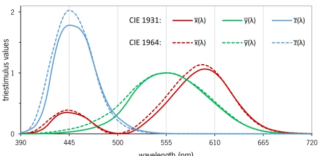
Tristimulus are colorimetric parameters that represent the magnitudes of the three primaries required to produce a specific color in additive mixing. The XYZ tristimulus are based on color matching functions 𝑥̅(𝜆), 𝑦̅(𝜆), 𝑧̅(𝜆) defined to produce imaginary tristimulus that reproduce all colors always assuming only positive values. The CIE recommends two sets of color matching functions [113], 𝑥̅(𝜆), 𝑦̅(𝜆), 𝑧̅(𝜆) and 𝑥̅₁₀(𝜆), 𝑦̅₁₀(𝜆), 𝑧₁₀(𝜆) (see Figure 1.6). These functions correspond to the CIE 1931 standard colorimetric observer and the CIE 1964 standard colorimetric observer. The data of the CIE 1931 standard colorimetric observer is intended for color stimuli subtending between about 1° and about 4° at the eye of the observer. The data of the CIE 1964 standard colorimetric observer should be used for visual angles larger than 4º.

Figure 1.6. Color matching functions 𝑥̅(𝜆), 𝑦̅(𝜆), and 𝑧̅(𝜆) of the CIE 1931 standard colorimetric observer (solid lines) and 𝑥̅₁₀(𝜆), 𝑦̅₁₀(𝜆), and 𝑧10(𝜆) of the CIE 1964 standard colorimetric observer (dashed lines) (adapted from [8,11].

The CIE 1931 XYZ tristimulus can be estimated using the following equations [113]: X = k ∑ ϕ(λ) ∙ x̅(λ)Δλ λ (1.1) Y = k ∑ ϕ(λ) ∙ y̅(λ)Δλ λ (1.2) Z = k ∑ ϕ(λ) ∙ z̅(λ)Δλ λ (1.3) 0 1 2 390 445 500 555 610 665 720 tri es timu lu s valu es wavelength (nm) x̅(λ) y̅(λ) z̅(λ) x̅(λ) y̅(λ) z̅(λ) CIE 1931: CIE 1964:

35

Where ϕ(λ) corresponds to the relative spectral radiance of the color stimulus for a given wavelength (λ). When necessary, radiance spectra of objects can be estimated from the multiplication between the relative spectral reflectance of the object R(λ) and the spectral radiance of the illuminating 𝑆(𝜆): ϕ(λ) = R(λ) ∙ S(λ).

The constant k is defined in a way that the tristimulus Y value of a Lambertian object (R(λ) = 1) is equal to 100. It can be obtained by the following equation:

k = 100/ ∑ S(λ) ∙ y̅(λ)Δλ λ

(1.4)

1.1.9.

CIELAB

CIELAB is a color specification system designed to match human visual perception. This space is fairly uniform, i.e. the colors tend to be distributed according to human perception and the approximated value of the difference between two colors can be obtained directly from the Euclidean distance between the points of space corresponding to those colors [113,114]. Figure 1.7 shows that the CIELAB system maps colors either by using three cartesian coordinates (L*, a*, b*) or by using cylindrical coordinates that are approximate correlates of the three perceived attributes of color: lightness (L*), chroma (C*ab), and hue (hab) [113,114]. The L* values are set

between 0 and 100, and all the space is defined so that the color of the illuminant is placed at the top of that scale.

Figure 1.7. Schematic representation of the coordinate system that make the tree-dimensional CIE 1976 (L*a*b*) color space (adapted form [115]).

hab

36

The CIE 1976 (L*a*b*) color space coordinates can be obtained from the CIE 1931 XYZ tristimulus by using the following equations [113]:

L∗ _{= 116 f (}Y Y_n) − 16 (1.5) a∗ = 500 [(X X_n) − f ( Y Y_n)] (1.6) b∗ _{= 200 [f (}Y Y_n) − f ( Z Z_n)] (1.7) 𝐶∗_𝑎𝑏= (a∗2+ b∗2)1/2 _(1.8) ℎ_𝑎𝑏 = arctan (b∗_/a∗_{) (1.9)} Where: 𝑓 (𝑋 𝑋_𝑛) = { (𝑋 𝑋_𝑛) 1 3 𝑖𝑓 (𝑋 𝑋_𝑛) > ( 24 116) 3 (841 108) ( 𝑋 𝑋_𝑛) + 16 116 𝑖𝑓 ( 𝑋 𝑋_𝑛) ≤ ( 24 116) 3 (1.10) 𝑓 (𝑌 𝑌𝑛 ) = { (𝑌 𝑌𝑛 ) 1 3 𝑖𝑓 (𝑌 𝑌𝑛 ) > (24 116) 3 (841 108) ( 𝑌 𝑌_𝑛) + 16 116 𝑖𝑓 ( 𝑌 𝑌_𝑛) ≤ ( 24 116) 3 (1.11) 𝑓 (𝑍 𝑍_𝑛) = { (𝑍 𝑍_𝑛) 1 3 𝑖𝑓 (𝑍 𝑍_𝑛) > ( 24 116) 3 (841 108) ( 𝑍 𝑍_𝑛) + 16 116 𝑖𝑓 ( 𝑍 𝑍_𝑛) ≤ ( 24 116) 3 (1.12)

Where X, Y, Z are the tristimulus values of the colored object in test. X_n, Y_n, Z_n are the tristimulus values of a Lambertian surface exposed to the same illuminant as the test object.

1.1.10.

Color ordered systems

A color ordered system is a color appearance system based on a collection of printed colored samples, arranged and labeled according to perceptual attributes of color to enable intuitive search and visual interpolation between samples [67,114,116–118]. These systems are typically used for identification of colors of objects without instrumentation by using only visual comparison. The Munsell Color System (MCS) and the Natural Color System (NCS) are two examples of such systems [114,119] (for more details on these systems see Chapter 2).

37

Chapter 2. Comparison between natural colors of the Minho

region and artificial colors of color ordered systems – Munsell

and NCS

38

2.1. Introduction

The chromatic gamut of printed color ordered systems is constrained by the limitations of the printing process [120]. Therefore, not all colors that may be important are in the printed catalogs. The Munsell Color System (MCS) and the Natural Color System (NCS) are two examples of such systems [114,119].

The Munsell system was devised by the artist A.H. Munsell in 1905 for color recording and color teaching [121,122]. It achieved an unmatched popularity by his contemporaries by successfully implementing three dimensions of color on a printed representation with uniform color scaling [123]. These three dimensions are expressed by the Munsell notation as Munsell value, Munsell hue, and Munsell chroma, and correspond respectively to the perceptual attributes of lightness, hue, and saturation [114,124]. The Munsell value of 0 is the ideal black and 10 the ideal white. On the Munsell Book of Color (MBC) the Munsell value is represented on a scale from 1 to 9 in steps of 1. This dimension is the axis around which the Munsell hue is established. The perceptual scaling of hue is done in circular steps between 10 major hues represented as 40 pages on the MBC. The major hues are referred as: Red (R), Yellow–Red (YR), Yellow (Y), Green–Yellow (GY), Green (G), Blue–Green (BG), Blue (B), Purple–Blue (PB), Purple (P), and Red–Purple (RP). The Munsell chroma is scaled from 0 to a maximum value that varies with the values of the two other dimensions. The system underwent several improvements over the years but the most notable one corresponds to adjustments on the correspondence between Munsell notation and printed samples [125]. This renotation was based on a study of over 3 million visual observations conducted by an OSA Subcommittee between 1937 and 1940 [126,127].

The NCS is a Swedish standard for color notation which was developed in 1964 by the Swedish Color Center Foundation [128]. The purpose was to make a practical model of the opponent-color theory conceived by the German physiologist Ewald Hering. Therefore, it consists on judging the appearance of a color by using two perceptual attributes of hue (chromaticness) and one of lightness (blackness). These are defined as the relative amount of red or green, the relative amount of blue or yellow, and the relative amount of black or white, respectively. Researchers involved reported that more than 60 thousand observations were made in psychophysical experiments based on the visualization of samples of colored papers [128]. These experiments served as guidance to produce a color atlas founded on the ideas of Hering. It was intended to represent every chromaticity at steps of 10% for blackness and for chromaticness for

39

40 different hues. This would result in 2000 samples but due to the pigments limitations this version (SIS Color Atlas NCS) was left with only 1412. Later more samples were added and the NCS ALBUM 1950 ORIGINAL with 1950 samples was achieved.

The colors of the natural world are produced by a range of physical and chemical phenomena that go behind the absorption of light by pigments, e.g. interference, diffusion and diffraction [129]. The colors that can be produced by pigments are represented by the object color solid, which is delimited by the optimal colors [34], but the real natural gamut is much smaller than this theoretical limit [5]. If the color ordered systems are designed to sample in a useful way the colors of the natural environment their colors should match as close as possible the structure of natural colors. The ideal color ordered system would have a chromatic gamut comparable to that of natural colors and their samples would be spaced to match the visual chromatic threshold. The goal of this work was to assess how well the MCS and NCS represent the colors of nature. We used spectral imaging of natural scenes (NS) and spectral data of these systems to render its colors under a range of different illuminants. The ability of the color ordered systems to represent natural colors was quantified in terms of chromatic volume and color difference between their colors and the natural colors.

2.2. Methods

The NS data set corresponds to about 68 × 106 pixels from 50 hyperspectral images of natural scenes of rural and urban outdoor environments from the Minho region of Portugal [130,131] obtained in the form of effective spectral reflectance from 400 nm to 720 nm, in steps of 10 nm. As effective spectral reflectances are obtained from a grey reference surface in the scene they need to be normalized to compute the corresponding colors in CIELAB. The reflectance array of each scene was normalized by dividing by a constant equal to the maximum effective spectral reflectance evaluated over all pixels and wavelengths in each scene (for technical details see [130]). This procedure guarantees that the reference white, a unitary spectral reflectance, is always the brightest surface in each scene.

The MCS data set corresponds to the 1269 color chips from the Munsell Book of Color - Matte Finish Collection (Munsell Color, Baltimore, Md., 1976) obtained from the online database of the University of Joensuu Color Group (Finland) [132]. Reflectance data was acquired from 380 nm to 800 nm in 1 nm steps.

40

The NCS data set corresponds to 1943 of the 1950 NCS standard color samples of the NCS ALBUM 1950 ORIGINAL (NCS - NATURAL COLOR SYSTEM, Scandinavian Color Institute AB, Stockholm, Sweden 2004). Each sample was measured using a portable spectrophotometer (CM-2600D, Konica Minolta, Japan) to obtain reflectance data from 400 nm to 700 nm in 10 nm steps with specular component excluded.

The illuminants used were 60 representing natural and artificial lighting: 55 CIE illuminants [113] and 5 white LEDs (Luxeon, Philips Lumileds Lighting Company, USA.). CIE Incandescent light: the CIE standard illuminant A correspondent to a tungsten filament at a temperature of 2856 K. CIE daylight illuminants: D50, D55, D65, D75 and other 19 D illuminants estimated from the correspondent CIE equations [113] (for a x coordinate value within the range of 0.3775 to 0.25 in steps of 0.0075 on the CIE (x,y)-chromaticity system). CIE fluorescent illuminants: FL1, FL2, FL3, FL4, FL5, and FL6 are traditional fluorescent lamps, FL7, FL8, and FL9 are broad-band, FL10, FL11, and FL12 are narrow band, FL3.1, FL3.2, and FL3.3, are standard halophosphate, FL3.4, FL3.5, and FL3.6 are DeLuxe, FL3.7, FL3.8, FL3.9, FL3.10, and FL3.11 are three band, FL3.12, FL3.13, and FL3.14 are multi band, and FL3.15 is a D65 simulator. CIE High-pressure illuminants: HP1 correspondent to a standard high-pressure sodium lamp, HP2 correspondent to a color enhanced high-pressure sodium lamp, HP3, HP4 and HP5 are typical high-pressure metal halide lamps. White LED illuminants: LXHL-BW02, LXHL-BW03, LXML-PWC1-0100, LXML-PWN1-0100, and LXML-PWW1-0060.

For the computations the NS and NCS reflectance data sets were interpolated to 5 nm to fit the spectral profile of some of the illuminants which present important peaks that would be overlooked if using a larger step. All computations were carried out between 400 nm and 700 nm in steps of 5 nm. Radiance spectra were estimated from the reflectance data by multiplying the spectral radiance of each illuminant spectrum. Assuming the CIE 1931 standard observer, the radiance data was converted into tristimulus values and then converted into the CIELAB color space. The reference white was assumed to be a sample with unitary spectral reflectance. The data points of NS, MCS, and NCS expressed in CIELAB assuming the illuminant D65 are represented in Figure 2.1.

To assess the extent to which the color ordered systems can represent natural colors we compared MCS and NCS data sets against the NS set in terms of chromatic volume and color differences. The volume and areas occupied by the NS set in CIELAB were estimated by convex

41

hull using the “convhull” function available in MatLab (MathWorks, Inc., Natick, MA, United States of America) based on the quickhull algorithm [133].

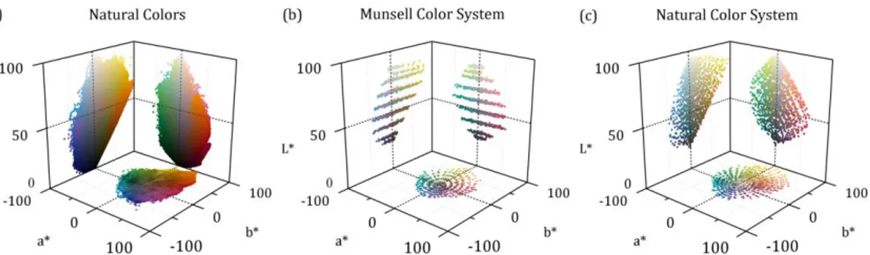
Figure 2.1. Representation of the natural colors obtained from spectral imaging (a), Munsell Color System (b) and Natural Color System (c) in CIELAB color space. Colors were computed assuming D65 illuminant. For illustration purposes only a fourth of the data points of (a) are represented.

The color difference ∆EL*a*b* between the colors of NS and each of the systems was estimated

by calculating the Euclidean distance between each natural color and the closest color in the color systems. Nearest neighbor calculations were implemented through the “nearestNeighbor” function available in MatLab (MathWorks, Inc., Natick, MA, United States of America) which resorts on Delaunay Triangulation. Because the color volume of the natural colors outgrows some portions of the volume of MCS or NCS, two subsets of natural colors were considered each including only the colors within the volume of MCS or NCS.

Figure 2.1 compares the color distributions of the three data sets. The MCS scatter is chromatically less dense, has 35% less data points than NCS. The MCS shows a more regular pattern than NCS and have distinct sub-sets of colors grouped at defined regions of the color space. In L*a* and L*b* planes MCS shows a well-defined pattern of 9 distinct clusters parallel to each other and to the a* and b* axes. Colors in the same cluster have similar L* and different saturations. These concentrated clusters are located on 9 different lightness levels set apart, on average, by 7.5 (±2.3) CIELAB units. This value was computed from the mean L* values estimated for the 9 clusters (26.2, 30.2, 39.3, 48.7, 57.8, 67.2, 76.6, 81.1, and 86.2 CIELAB units) through clustering analysis based on the Lloyd’s algorithm [134] and k-means++ algorithm [135] by using the “kmeans” function available in MatLab (MathWorks, Inc., Natick, MA, United States of America). These levels correspond to the 9 levels of grey on the notation scale of Munsell value. On the hue plane a*b* MCS presents a pattern of well-defined concentric circles indicating that MCS has larger sampling steps on saturation than on hue. These data are generally consistent

42

other studies involving the chromatic structure of the 1269 Munsell Samples [136]. The NCS scatter on L*b* has a more homogeneous appearance with a less perceptible structure pattern.

2.3. Results

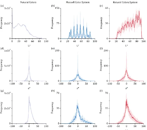
Figure 2.2 shows that both color systems offer more color samples of low saturation matching the saturation distribution of the natural colors. The L* distributions of the three data sets, however, are distinct. Figure 2.2 (a) shows that natural colors have higher frequency in the lower half of the L* axis. The bin of L* from 0 to 1, corresponding to points of extreme shadow, has the highest frequency and presents a protruding peak. These points correspond to regions of almost complete darkness that are mostly found in distant areas under shadow, cracks of surfaces, and empty space between agglomerates of objects (e.g. plant leaves) where the illuminant light cannot penetrate and be reflected.

Figure 2.2. Color distributions of the three data sets. Colored solid lines represent mean frequency of colors across 60 illuminants and the corresponding range for the illuminant set (colored shaded area).

43

Figure 2.2 (b) and (c) show that the MCS system has more data points on median levels of L* whereas the NCS shows a preference for higher levels of L*. For MCS and NCS the lightness levels for the mean illuminant range from 22 to 91 and from 18 to 96, respectively (Figure 2.2 (b) and (c), colored solid lines). These intervals do not cover the full extent of the natural colors, particularly for L* lower than around 20 CIELAB units. Natural colors are more frequent on this low lightness region than on the high lightness one. Thus, the color systems cover the ranges of L*, a*, and b* on natural colors distribution with higher frequency, but for L* some portions are underrepresented. Figure 2.2 shows the colored shading areas corresponding to the range of illuminants tested. The variability is modest. The mean and the D65 data are similar in all cases, and most of the variability on a* is caused by the illuminant HP1.

Figure 2.3. Results of the convex hull and point analysis. (a) The CIELAB diagram represents for the CIE standard illuminant D65 the convex hulls of the natural colors (grey solid line), MCS (blue solid line), and NCS (red solid line). (b) Fraction of the volume and areas of natural colors occupied by the color systems. (c) Fraction of the natural colors inside each color system. (b) and (c) represent mean data across the illuminants set.

Figure 2.3 shows the results of the convex hull and point analysis. Figure 2.3 (a) compares the convex hulls between the data sets for D65. The volume of natural colors outgrows the volume of both color systems. The MCS has smaller volume than NCS, covering 71,5% of the NCS volume.

44

2.5% of NCS colors are outside the volume of natural colors. Figure 2.3 (b) shows the mean volume and mean area of the color systems relatively to natural colors. The MCS and NCS relative volumes are 37.7% (±3.4) and 52.7% (±4.6), respectively. Figure 2.3 (c) shows the fraction of natural colors inside MCS and NCS color volumes, about 37.6% (±0.1) and 44.9% (±5.8), respectively.

Figure 2.4 (a) and (c) show the results of the color difference analysis. The MCS and NCS mean distributions present peaks at ∆EL*a*b* 25.0 and 18.6 CIELAB units, respectively, as a result

of the dense agglomeration of natural colors near the origin of the CIELAB color space (see Figure 2.2 (a), (d) and (g)). Figure 2.4 (c) shows that a visual perfect match for all natural colors requires an observer with chromatic threshold of 25.0 and 19.2 CIELAB units for MCS and NCS, respectively.

Figure 2.4. Results of the color difference analysis. (a) and (c) Represent the relative frequency and cumulative frequency, respectively, of color differences expressed in CIELAB between each natural color from the set of natural scenes (NS) and the corresponding one in the MCS or NCS. (b) and (d) Represent similar data but for the subset (NS’) of the natural colors which includes only data points within the volume of each color system. Data represent mean across illuminants for MCS (blue solid line) and NCS (red solid line) and corresponding range across illuminants for MCS (blue shaded area) and NCS (red shaded area).

45

Figure 2.4 (b) and (d) present similar data but for the NS’ set that corresponds to the natural colors within the volumes of each color system. Figure 2.4 (b) shows that the most frequent ∆EL*a*b*

value across illuminants is on average 3.0 and 2.2 CIELAB units for MCS and NCS, respectively. Figure 2.4 (d) shows the corresponding cumulative frequency. For an observer with a chromatic threshold of 1 CIELAB unit 6.7% and 6.9% of the NS’ colors will look the same as the correspondent MCS and NCS samples. For a chromatic threshold of 2 CIELAB units 26.3% and 34.2% of the NS’ colors will look the same as the correspondent MCS and NCS samples, respectively. Figure 2.4 (d) also shows that the threshold needed to achieve color match on NS’ colors would be on average 6.8 and 5.4 for MCS and NCS, respectively.

The distributions are similar across illuminants, except for HP1 which has its most frequent

∆EL*a*b* value significantly lower than the most frequent value for the mean distribution. For HP1,

the most frequent ∆EL*a*b* value is only 1.4 and 1.6 for MCS and NCS, respectively. Match for all

NS’ colors is achieved with thresholds of 4.8 and 4.2 for MCS and NCS, respectively. The chromatic volume produced by this illuminant is contracted across the a* axis resulting in small values of relative volume (33.1% and 47.9% for MCS and NCS, respectively) while covering a reasonable portion of NS points (37.7% and 46.0% for MCS and NCS, respectively). This indicates that for HP1 a stronger concentration of natural colors occurs inside the zones of the color space occupied by the color systems, decreasing the distance between the NS data points and the correspondent color systems data points.

The analysis was complemented with Voronoi diagrams to study how ∆E varies across color space. Voronoi decomposition of MCS and NCS for each CIELAB plane (a*b*, L*a*, and L*b*) was carried out by using “voronoin” function available in MatLab (MathWorks, Inc., Natick, MA, United States of America) which is based on the quickhull algorithm [133]. The Voronoi decomposition defines for each color system data point the boundaries of a polygonal area that only includes the points of space closer to that data point than to any other data point. Thus, each polygonal area represents the chromatic territory of a color system sample and is color coded for the mean value of color difference (∆Ea*b* or ∆EL*a* or ∆EL*b*) between the COS data point and each NS data point

enclosed by that area.

Figure 2.5 shows how color difference vary across the CIELAB planes by using Voronoi diagrams mapping ∆E values computed for a*b*, L*a*, and L*b* color spaces. What is represented

46

is the color difference between each natural color and the corresponding color of MCS (a) and NCS (b). Data corresponds to the chromaticity coordinates of Figure 2.1, i.e. assuming D65 as the illuminant. For the majority of the Voronoi cells the mean ∆E values seem to range from around 0 to 3, which agrees with the greatness of values of ∆EL*a*b* in Figure 2.4. Voronoi diagrams for NCS

are overall more uniform and present lower mean ∆E, in particular for data points close to the achromatic locus. The a*b* diagram of MCS shows larger color differences for positive values of b* than for negative values and the diagrams L*a* and L*b* of MCS show irregularities across the color space that are consistent with the scatter pattern of MCS shown in Figure 2.1. In both color systems ∆Ea*b* tends to be larger for more saturated colors.

Figure 2.5. Variations of ∆E color differences between the COS and natural colors across the color space. Voronoi diagrams map ∆E values for a*b*, L*a*, and L*b* between each natural color and the corresponding color of MCS (a) and NCS (b). Data corresponds to the colors of Figure 2.1 assuming D65 illuminant.

47

2.4. Discussion

The portion of the volume of the natural colors accounted by MCS and NCS was about 38% and 53%, respectively. The color ordered systems do not include mainly colors with low lightness, which are frequent in natural scenes. Apart from the dark colors both color systems are a good match to the natural colors, especially for non-saturated colors.

The NCS has a lower average color difference in relation to the natural colors than MCS, i.e., on average for each natural color there is a color in the NCS system that is visually closer than a color in the MCS. For an observer with a color threshold of 1 CIELAB unit only about 7% of the natural colors have a corresponding color (perceived as the same) both in MCS and NCS. For a threshold of 2 CIELAB units the percentage is 25% and 19% for MCS and NCS, respectively. To obtain a complete match to all natural colors contained by the color systems volumes thresholds of 7 and 5 CIELAB units would be required for MCS and NCS, respectively. For the complete set of natural colors thresholds of about 25 and 20 for MCS and NCS, respectively, would be required. The NCS has some very saturated colors that are outside the volume of natural colors and therefore represent colors that are not frequent in nature.

The computation of natural colors in CIELAB color space were carried out assuming that the reference white is he brightest color in each scene. Although this is a reasonable assumption it may not hold for all viewing conditions. In practice, however, it will work well in most conditions. The computations also do not take into account the variation of the illumination across scenes which can be considerable [137]. The computations for different illuminants, however, suggest that these variations have a small effect in the conclusions.

The results presented here suggest that both color systems are limited at representing the natural colors with low lightness levels. They are, however, quite good otherwise. The ideal color ordered system for describing natural colors would need a chromatic gamut covering the saturation levels, for a* and b*, between about -100 to 100 CIELAB units and include all levels of lightness. Its samples would need to be evenly distributed in a step corresponding to the discrimination threshold of the observer in a way that all natural colors would have a perfect color match on the correspondent sample.

Using the Munsell system or the NCS as models of the colors of the natural world may be insufficient in some cases and more complete spectral data may be necessary.

48

In regard only to the analysis on Minho’s natural scenes, the results show that natural colors can assume very saturated colors but that these are very rare. In the natural scenes is possible to find colors of almost any possible level of L*, but bellow lightness level of 50 CIELAB units is contained about 90% of the natural colors.

49

Chapter 3. The colors of natural scenes benefit dichromats