www.scielo.br/rbg
GEOTECHNICAL DESCRIPTION OF SANDY SEDIMENTS OF THE SURF ZONE
USING ELECTRICAL RESISTIVITY MEASUREMENTS
Fernando Rocha Carneiro
1, Arthur Ayres Neto
2,
Rodrigo Menezes Raposo de Almeida
3and
Sidney de Matos Mello
4ABSTRACT.The geotechnical description of sandy sediments of the surf zone was done in two ways: directly, through standard geotechnical testing proposed by ASTM (American Society for Testing and Materials) and indirectly, through electrical resistivity measurements. The geotechnical property chosen for the description of the sediment was porosity, due to its influence in a wide range of soil properties. The indirect estimate of porosity through resistivity measurements was based on Archie’s equation. However, the difficulty in generalizing this equation is the empirical determination of the cementation exponent (m). For this reason, the values proposed by other authors were tested. A comparison of the porosity values obtained by the two methods (directly and indirectly using different values for cementation exponent) showed that it is not advisable to use cementation exponent (m) from other authors indiscriminately. Moreover, the application of the porosity values obtained by the ASTM tests allowed calculating a more suitable cementation exponent value for sandy sediments of the surf zone (between 1.48 and 1.79). Besides porosity, other geotechnical parameters, such as void ratio (e) and total density (ρt), were also differentiated by measuring the electrical resistivity of selected samples allowing
to describe the geotechnical state of the sediment with higher confidence.
Keywords: electrical resistivity, coastal engineering, Archie’s equation, porosity, grain size.
RESUMO.A descrição geotécnica dos sedimentos arenosos da zona de arrebentação foi feita de duas maneiras: diretamente, através de ensaios geotécnicos padrão, propostos pela ASTM (Sociedade Americana de Testes e Materiais) e indiretamente, através de medidas de eletrorresistividade. A propriedade geotécnica escolhida para a descrição do sedimento foi a porosidade, por ser uma variável importante na caracterização das propriedades do solo. A estimativa indireta da porosidade através de medidas de resistividade foi baseada na equação de Archie. Entretanto, a principal dificuldade em generalizar esta equação é a determinação empírica do expoente de cimentação (m). Por esse motivo, os valores propostos por outros autores foram testados. Uma comparação dos valores de porosidade obtidos pelos dois métodos (direta e indiretamente, usando diferentes valores para o expoente de cimentação) mostrou que não é aconselhável usar expoente de cimentação (m) de outros autores indiscriminadamente. Além disso, a aplicação dos valores de porosidade obtidos pelos testes ASTM permitiu o cálculo de um valor para o expoente de cimentação mais adequado para sedimentos arenosos da zona de arrebentação (entre 1,48 e 1,79). Além da porosidade, outros parâmetros geotécnicos, como índice de vazios (e) e densidade total (ρt), também foram diferenciados pela medição da resistividade elétrica de amostras selecionadas, permitindo descrever o estado geotécnico do
sedimento com maior confiança.
Palavras-chave: eletrorresistividade, engenharia costeira, equação de Archie, porosidade, granulometria.
1Universidade Federal Fluminense, Postgraduate Program in Dynamics of Oceans and Earth, Av. General Milton Tavares de Souza S/N - Niterói/RJ, Brazil - E-mail:
2Universidade Federal Fluminense, Geology and Geophysics Department, Av. General Milton Tavares de Souza S/N - Niterói/RJ, Brazil - E-mail: [email protected] 3Universidade Federal Fluminense, Geotechnology Laboratory, School of Engineering, Av. General Milton Tavares de Souza S/N - Niterói/RJ, Brazil - E-mail:
4Universidade Federal Fluminense, Geology and Geophysics Department, Av. General Milton Tavares de Souza S/N - Niterói/RJ, ZIP Code: 24210-346, Brazil - E-mail:
INTRODUCTION
The goal of the Brazilian government to expand oil exploration in the pre-salt reserves, area that extends from the state of Santa Catarina to the state of Espírito Santo, southeastern Brazil, motivated this study, since it will demand many infrastructure projects along the coast.
One of the challenges of this expansion will be the creation of pipelines responsible for the flow and distribution of oil and gas from the production areas in the offshore fields to the continent. In this context, geophysical, geotechnical and oceanographic surveys are fundamental in stages prior to the installation of offshore pipelines (Azevedo et al., 2005; Solano et al., 2005; Teixeira et al., 2005).
Nowadays pipeline engineering uses acoustic geophysical methods to characterize the seabed prior to the installation of a pipeline, with multibeam echo sounder, side scan sonar and the sub-bottom profiler being the most used systems. Each of these devices has a different goal: the multibeam echosounder maps the seabed’s morphology, the side scan sonar provides information related to the geology of the seabed and the sub-bottom profiler allows to obtain information on the structural arrangement of the geological layers in the subsurface.
The integration of these informations associated with the collection of geotechnical and geological samples provide enough subsidies for the installation of a pipeline. However, this is not true for the surf zone. This area is represented by a narrow band where the waves break due to reduction of depth to a value less than or equal to the wave base (Suguio, 2003).
This area, being restricted to navigation because of waves and currents regime and shallow depths, limits the access of survey vessels. Another problem in this area is the fact that the air bubbles created by breaking waves produce noise on acoustic records (Tang et al., 1994; Boyle & Chotiros, 1995; Tang, 1996; Chu et al., 1997; Fonseca et al., 2002), thus compromising the quality of the data and the effectiveness of these methods.
For these reasons, the surf zone is currently considered a ”blind zone” for traditional marine geophysical methods, representing a gap of information in most surveys in coastal areas.
The motivation of this study was to investigate alternative tools for collecting geotechnical information about this area to assist pipeline engineering projects. According to Valent (1974) the knowledge of porosity and in situ density is essential for predicting the seabed behavior when a load is applied to it, which
means it is very important to estimate these parameters before the engineering process is installed.
In the case of sandy bottoms, which do not allow deformation-free sampling due to its geometrical instability, indirect methods such as resistivity measurements may be used to estimate geotechnical properties (Jackson et al., 1978).
In this study, in addition to the electrical resistivity, the samples were also tested in laboratory for water content, total density, void ratio and porosity following procedures proposed by ASTM (American Society for Testing and Materials). The comparison of the results between the two methods ensured the validation and adjustment of the results.
The water content of each sample was defined as the ratio between the water mass and the dry solids mass Germaine & Germaine (2009).
ωc= Mu Ms
× 100, (1)
where:ωc– Water content [%]; Mu– Mass of water [kg]; Ms– Mass of dry soil [kg]. In this study we used the total density for geotechnical sample description, which is defined by soil mass per volume unit.
ρt= Ms
Vt
, (2)
where:ρt– Total density [g.cm−3]; Vt – Total volume [cm−3] According to Schopper (1982), the void ratio quantifies the space available for soil compression or flow, Eqs. (3) and (4), and is geologically known as intergranular porosity, defined as the gap between the clastic fragments occupied by gases or fluids in unconsolidated, compressed or cemented sediment. It is also called primary porosity.
e=Vv Vs
, (3)
where: e – Void ratio [dimensionless]; Vv – Volume of voids [m−3]; V
s– Volume of solids [m−3] n=Vv
Vt
, (4)
where: n – Porosity [dimensionless].
These geotechnical properties define the state of a geo-material when it comes to soft soils and are better descriptors for saturation and water content. Density, on the other hand, is more applied to compacted soils and rocks. Void ratio (e) or porosity (n) are the most universal measures and are applicable to different types of soil Germaine & Germaine (2009). For this
reason porosity was the geotechnical property chosen to be estimated by electrical measurements.
Using Archie’s law it was possible to correlate the porosity (n) with the electrical resistivity of the samples. Archie empirically established that the resistivity in water-saturated clean sediments is proportional to the electrical resistivity of the interstitial water itself. As a result, Chen et al. (2008) obtained:
F=Rsed Rpw
, (5)
where: F – Formation factor [dimensionless]; Rsed– Resistivity in water-saturated sediment [ohm.m]; Rpw – Resistivity of pore water [ohm.m].
After reading different sandstone samples, an exponential relation was established between the values of the formation factor and the porosity (n) of each investigated formation (Chen et al., 2008), reaching:
F= n−m,
(6) where m – cementation exponent [dimensionless].
Archie’s law has become the most common method used to relate the porosity of a reservoir rock and the conductivity of interstitial fluid for more than 60 years. This is due to the fact that an empirical relationship applied to a small group of rocks with specific porosity can be widely used, especially in the petroleum industry (Glover, 2010).
The electrical resistivity of saturated sediments is complicated due to the complex framework formed by the grains. In general, the grain matrix is nonconductive, i.e., its electrical resistivity is much greater when compared to the interstitial electrical resistivity of the pore fluid. Therefore, the electrical conduction occurs primarily through interstitial water (Boyce, 1968). The exception is when the sediments have some amount of clay fraction. Clay minerals, due to their negative electrostatic charge act as semi-conductors.
The premise of the electrical conductivity being essentially a function of the interstitial fluid is applicable to the samples of this study, since its mineralogical composition is mainly (< 97%) quartz with very small amounts of biodebris (essentially shell fragments). These form a framework of nonconductive grains, as quartz minerals are considered insulators in saturated marine sediment samples (Archie, 1942).
Studies involving the subject basically use resistivity values to express the electrical characteristics of saturated soils, which enables the calculation of the formation factor (F) by Eq. (5). The formation factor expresses the effects of the resistivity of the matrix grains and allows the calculation of the porosity
(n) by using Eq. (6). The greatest difficulty in the porosity calculation using this method involves the determination of the empirical constant m, also known as cementation exponent. Values proposed by other authors, such as Doveton (1986), Jackson et al. (1978) and Keller (1989), were used in order to determine which of them would fit better to the samples of used in the present study.
The main objective was to compare the porosity values obtained directly from laboratory tests with those obtained indirectly using electrical resistivity measurements calculated by Eq. (6), and by that, determining how much this indirect estimation is accurate in sandy sediments from the surf zone. Another important point of this study is that the samples in which the electrical measurements were obtained were divided into two groups, the first representing the most compact state (minimum void ratio), and the second representing the less compacted state (maximum void ratio). The comparison between the values would indicate the sensitivity of the proposed technique to variations of porosity and, therefore, density and degree of compaction, both within the same sedimentary material. This comparison would indicate an interesting measure for pipeline engineering, as the sand compression capacity, is a very important information for the installation of any subsea facility.
The application of Archie’s law (Eq. 6), using the porosity values obtained in laboratory, resulted in the calculation of a new empirical cementation coefficient (m). Different studies have correlated m to the porosity of sedimentary materials and found no significant relationship. This confirmed the assumption that m is preferentially linked to the geometry of the pores and not to the volume of interstitial water in the sediment.
Furthermore, m contains additional information about the sedimentary package texture (Schön, 2015). The influence of texture on the exponent is the physical basis used in the studies to find a relationship between the cementation exponent (m) and permeability (Schön, 2015). Studies conducted by Glover et al. (2006) have proposed a model to estimate the permeability of a formation from a relationship with the cementation exponent, known as RPGZ model.
k= d 2n3m
4 pm2, (7)
where: k – Permeability [m2]; p – Packing parameter [dimensionless]; d – Effective grain diameter [m]; m – Cementation exponent [dimensionless]; n – Porosity [dimensionless]
The m values obtained in our study were used to calculate the permeability of sediment samples and the results were compared with those obtained by Glover et al. (2006).
MATERIAL AND METHODS
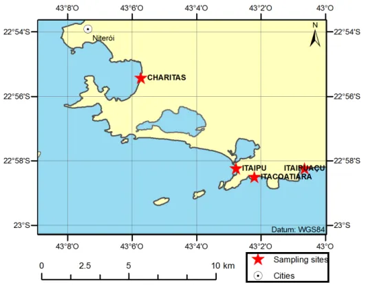
Sediments were collected in surf zones of four beaches in the cities of Niterói and Maricá, state of Rio de Janeiro (showed in Fig. 1), SE Brazil: Itacoatiara (medium sand), Charitas (fine sand), Itaipuaçu (very coarse sand) and Itaipu (medium sand). The choice of samples covering a wide range in the granulometric scale is justified since particle size variations reflect changes in the geotechnical properties of the sediment, especially porosity and compaction degree (Hartge & Horn, 1999).
The samples were firstly submitted to dry sieving and the weights of each fraction placed in GRADSTAT software for the calculation of statistics and granulometric parameters. Among all the methods used by the software, it was chosen as standard for this study the measurements obtained by the Folk & Ward (1957). It is noteworthy that the samples did not undergo any process for removal of carbonate, i.e., all granulometric parameters considers the presence of biodebris.
To each of the four sampling sites two samples (1 and 2) were prepared with the volume of 2.4 liters of sediment, one representing the most dense state (minimum void ratio) that the grains could theoretically assume and the other, the less dense state (maximum void ratio).This was done by following the methods ASTM D4254 Minimum Index Density and Unit Weight of Soils and Calculation of Relative Density, Method C and ASTM D4253 Maximum Index Density and Unit Weight of soils using a Vibratory Table.
The method for constructing the sample probes with different densities is applied to dry soil samples, but for future steps it is essential to have the sediment 100% saturated with sea water. This process required an adjustment in sample tubes, with the installation of taps on the lower ends of tubes, allowing the injection of water, and a valve on the upper end allowing the air to escape.
Another concern during this step was that the injection of water in the sample could change the density structure of the sample. In order to minimize these disturbances caused by the inflow of water, a gravel layer was introduced at the base of the sample in order to dissipate the energy of the inflow before it reaches the sample itself. Another objective of this filling
sequence is to seal the sample in the central part of the corer, preserving to the maximum the density structure of the sediment sample.
The electrical properties of the test specimens with different degrees of compression were determined using the Non-Contact Resistivity Sensor (NCR) of multisensor Core Logger (MSCL) from Geotek (Geotek, 2014), an equipment that only accepts samples 100% saturated with water.
NCR technique works from a transmitting coil which emits a magnetic field of high-frequency in the corer, inducing electrical currents that are inversely proportional to the resistivity. These currents generate small magnetic fields which, in turn, are measured by a receiving coil. To measure such small values with a certain precision and accuracy, this technique compares the differences between the measurements obtained by the receiving coils with an equal operating assembly exposed to air, with zero resistivity. For this reason, to achieve readings between 0.1 and 10 ohm-meter with a 0.5 cm vertical resolution throughout the corer, samples should be 100% saturated without the presence of air bubbles (Geotek, 2014).
Before reading the sediment samples, the resistivity sensor has undergone a calibration process, which consists in reading a sequence of samples of water with a known salinity. With these measurements, a calibration curve is constructed and applied to the raw data in order to convert them from tension measurements (mV) for electrical condutivity measurements (Sm−1) and its inverse, the resistivity (ohm.m). Another important point that also ensures the quality of the data is the fact that all samples had replica, the end result being an average between the two measurements.
From the geological point of view, the resistivity measurements consist of impedance measurements, with subsequent interpretation in terms of the electrical property of
the subsurface geological structure, based on the response of each material to the flow of an electric current (Ward, 1990). Using Archie’s law, we can translate those electrical variations as a function of the geological structure in tangible values, such as porosity.
Porosity was also estimated by geotechnical testing, as well as water content (ωc), total density (ρt) and void ratio (e), all following the methods proposed by ASTM. Laboratory tests are based on the relationship of volume and weight of the different phases of the samples, namely the solid phase, represented by the granular framework, and the liquid phase represented by the interstitial fluid.
As sediments are not geometrically stable, this term refers to soil samples that are not able of maintaining the shape. This fact makes it difficult to calculate the ratios of volumes between the two phases (Germaine & Germaine, 2009). Once the volumes are known, with few simple calculations we can extract porosity and void ratio using Eqs. (3) and (4), wherein the porosity expresses the voids relative to the total volume, while the void ratio is related to the volume of grains. This difference makes the void ratio more useful when working with calculations of tension. However, the porosity is more applicable to situations involving flow, because it is directly related to the space available for flow (Germaine & Germaine, 2009).
RESULTS
Grain size analysis and geotechnical testing
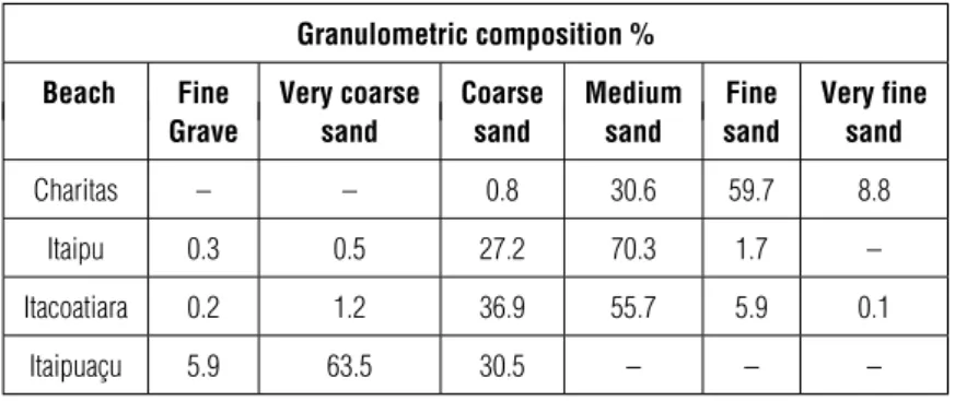
The first results obtained in the laboratory were the grain size values, as shown in Table 1. The sediments vary from very fine sand to fine gravel, according to the classification of Folk & Ward (1957).
Sediments collected in the surf zone have quartz as the main mineralogical composition, although in Itacoatiara there Table 1 – Granulometric composition
Granulometric composition %
Beach Fine Very coarse Coarse Medium Fine Very fine
Grave sand sand sand sand sand
Charitas – – 0.8 30.6 59.7 8.8
Itaipu 0.3 0.5 27.2 70.3 1.7 –
Itacoatiara 0.2 1.2 36.9 55.7 5.9 0.1
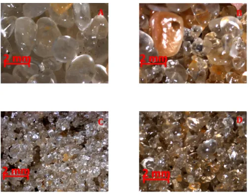
Figure 2 – Photos of the studied samples showing the roundness an grain size of the sediments (A – Itaipuaçu beach; B
– Itacoatiara beach; C – Charitas beach; D – Itaipu beach).
Table 2 – Mean values of the geotechnical parameters for each sample site.
Geotechnical Parameters
Beach Average Diameter Porosity Void ratio Water Content Density
(µm) (n) (e) (W%) (g/cm3)
Charitas 207.5 0.406 0.684 14.9 1.89
Itaipu 447.4 0.368 0.583 12.2 1.96
Itacoatiara 447.4 0.358 0.559 11.4 1.99
Itaipuaçu 1179.9 0.335 0.505 8.6 1.99
is an important biogenic component consisted of biodebris. In the classification of Folk & Ward (1957) all samples were classified as symmetrical and the degree of selection varied between moderately well-selected and selected.
Figure 2 shows sediment photos of the four samples. As expected, the sediments are well rounded in all samples, i.e., few angular grains.
The granulometric analysis is closely related to the geotechnical data, and the results of the weights and volumes of the two phases comprising the sample allowed the calculation of
some geotechnical properties using Eqs. (1) to (4). The values are presented in Table 2.
The maximum average porosity was 0.406±0.010 (40.6%) for the samples from the Charitas beach, while the minimum average porosity was 0.335±0.021 (33.5%) for the samples from Itaipuaçu beach. The other geotechnical parameters show the same behavior as porosity, having its maximum for the samples from Charitas beach (finer sand) and its minimum for the samples from Itaipuaçu beach (coarser sand). Density is the only parameter that presents a reverse behavior, with its maximum
for the samples from Itaipuaçu beach and its minimum for the samples from Charitas beach.
This result was expected since, the larger the voids, the greater the volume of water in the sample and lower the overall density.
The void ratios values can be extracted from the porosity values using the following equation:
e= n
1 − n, (8)
Porosity determined by electrical resistivity measurements
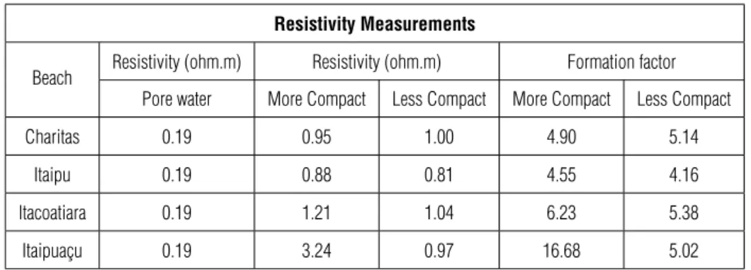
On the other hand, porosity values were calculated using electrical resistivity measurements at the MSCL. Specimens from both groups of samples were logged by the sensor, estimating resistivity values in ohm.m for each samples (Table 3).
The resistivity values ranged between 3.24±0.16 ohm.m and 0.81±0.075 ohm.m for the densest Itaipuaçu sample and the less dense Itaipu sample, respectively. The sample with the highest standard deviation between replicates was Charitas less dense sample, 0.99±0.32 ohm.m−1.
The results are consistent with the values found for non-consolidated sandy sediment samples in other studies (Boyce, 1968; Ayres Neto, 1998). These values were converted to formation factor (F), a non-dimensional number that represents the ratio between the saturated sediment resistivity and the interstitial fluid resistivity, Eq. (5).
The results for the formation factor (F) followed the same trends of the electrical resistivity. The was applied in Eq. (6) for the estimation of porosity with different cementation exponent values (m) proposed by other authors.
According to Schön (2015), the value proposed by Doveton is more general and can be used for unconsolidated sediments,
being the value proposed = 1.3. On the other hand, the value proposed by Jackson et al. (1978) is more restrictive, being applicable to sands with porosity lower than 0.60 (60%). In the study conducted by Keller (1989), the formation factor value is specifically applied to sedimentary packages with low degrees of cementation, particularly sandstones with porosity between 25% and 45%. Furthermore, he introduces a change in the original Archie’s equation with the addition of a new constant, with which the Eq. (6) becomes:
F= anm, (9) where: a – Empirical constant [dimensionless].
Keller (1989) proposed values for a = 0.88 and m = 1.37. Although the constants have been calculated for consolidated sediment (sandstone), the unconsolidated sediment samples in this study may have similar behavior, since the laboratory conditions allowed the construction of samples with controlled degree of compaction and restricted volume. For these reasons, it is expected that the results should be similar to sandstones with same mineralogical composition, justifying the use of these values and the Eq. (9).
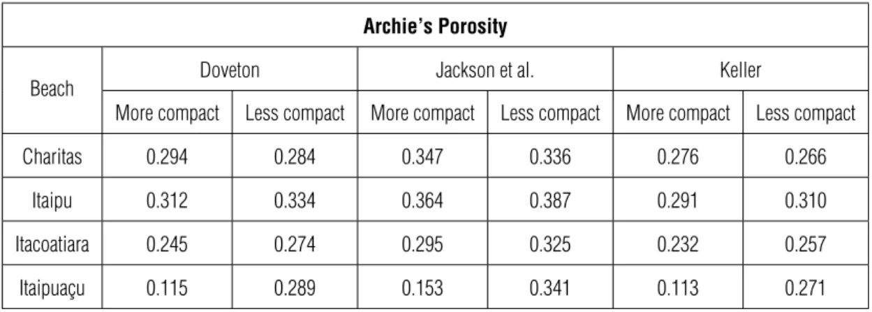
The results for porosity obtained using the three constants followed the same trend. The lowest porosity were determined using the cementation exponent value proposed by Keller (1989). The intermediate and highest values were determined using m value proposed by Doveton (1986) and Jackson et al. (1978), respectively (Table 4).
When comparing the two groups of samples it was observed that the less compact samples presented higher porosities, while the more compact showed the lowest porosity values. The exception to that expected rule was represented by the samples from Charitas, where the more compact samples showed higher porosities.
Table 3 – Resistivity values and formation factor for the two groups of samples.
Resistivity Measurements
Beach Resistivity (ohm.m) Resistivity (ohm.m) Formation factor
Pore water More Compact Less Compact More Compact Less Compact
Charitas 0.19 0.95 1.00 4.90 5.14
Itaipu 0.19 0.88 0.81 4.55 4.16
Itacoatiara 0.19 1.21 1.04 6.23 5.38
Table 4 – Values of porosity calculated by variation of the Archie’s law according to Doveton (1986), Jackson et al. (1978) and Keller (1989).
Archie’s Porosity
Beach Doveton Jackson et al. Keller
More compact Less compact More compact Less compact More compact Less compact Charitas 0.294 0.284 0.347 0.336 0.276 0.266
Itaipu 0.312 0.334 0.364 0.387 0.291 0.310 Itacoatiara 0.245 0.274 0.295 0.325 0.232 0.257 Itaipuaçu 0.115 0.289 0.153 0.341 0.113 0.271
In order to compare the porosity values determined directly through the ASTM tests and indirectly through the electrical resistivity measurements, it was necessary to calculate the average porosity values between the more and the less compact sample. This was done because the laboratory values are an average of the primary porosity (Table 5).
As shown in Table 4, the most compact sample from Itaipuaçu beach presented an anomalous high porosity value. The variation in porosity between the two groups for the same sample ranged between 3.14% and 11.6% for three of the four samples, except Itaipuaçu, where the variation reached 86.3%. For this reason, only the values calculated for the least compacted sample was used.
Table 5 – Average porosities after Doveton (1986), Jackson et al. (1978), Keller
(1989) and ASTM.
Average Porosities
Beach Doveton Jackson et al. Keller ASTM Charitas 0.289 0.341 0.271 0.406 Itaipu 0.323 0.375 0.301 0.368 Itacoatiara 0.259 0.310 0.245 0.358 Itaipuaçu 0.289 0.341 0.271 0.335
The comparison between two groups of samples showed that the most appropriate value m would be the one suggested by Jackson et al. (1978).
The same procedure was done for the formation factor values. The average values of formation factor were associated to the average primary porosity values obtained in laboratory (Table
2 and 3), allowing the calculation of a new m for each sample using Eq. (6).
Differences between the constants determined by Doveton (1986), Jackson et al. (1978) and Keller (1989) and those calculated in this study are a good indication of the influence of using inappropriate m values. The greater the difference, the greater would be the the error in the porosity values.
The cementation exponent (m) is interpreted as the change rate of the connection between pores as a function of porosity and pore arrangement (Glover, 2009). The connection between pores indicates the space available to the pore fluid and electric current to flow, which is closely linked to the permeability of the sedimentary package. Isolated pores do not participate in permeability, or in the electrical conductivity of the sediment.
The results were applied in Eq. (7) for the calculation of permeability following the RPGZ model. According to Campanya et al. (2015) for the model to be valid, certain conditions must be observed:
- The grain size is larger when compared to the difference between the average and maximum or minimum of the effective radius of the grain;
- The m and F values are derived from the pore water; - The formation factor is always greater than 1; - The model has no limit in the porosity values.
Obeying these conditions the permeability values were calculated as indicated in Table 6.
The permeability data are consistent with those found by Glover (2009) in sandstones. According to Glover (2009), higher permeability values are related to samples with larger grain sizes, as they have larger pores.
Table 6 – Results of RPGZ model for permeability and parameters used for the calculation.
Average Permeability
Beach Mean Diameter (µm) Porosity (n) Cementation Exponent Permeability (k.10−12)
Charitas 127.1 0.406 1.79 3.74
Itaipu 302.5 0.368 1.47 47.97
Itacoatiara 266.1 0.358 1.71 11.56
Itaipuaçu 752.7 0.335 1.48 192.00
DISCUSSION
The results obtained by the granulometric analysis followed the expected pattern and fulfilled the goal of choice for samples that covered a wide range of particle size. The objective was to obtain remarkable differences in the geotechnical characteristics among the samples, making the study applicable to a wider variety of sediment types.
Visual analysis of the samples showed well-selected sediments with a high degree of rounding. These features reflect the dynamic conditions of the surf zone, characterized by high energy (waves and currents), which increase the friction and abrasion between the sediment grains, making them more rounded.
The grain size and visual analysis of the samples served as basis for the interpretation of the electrical and geotechnical properties of the sediment samples.
The analyzed geotechnical properties (porosity, void ratio, water content and total density - Table 2) were important for the validation of the indirectly estimated porosities following Archie’s law. Moreover, in order to ensure the reliability of the laboratory tests results, these values were compared to Hamilton & Bachman (1982) study, who used the same method to calculate the porosities and densities in unconsolidated marine sediment samples.
Hamilton & Bachman (1982) study showed porosities and densities ranging between 37% to 57% and 2.034 g.cm−3 to 1.878 g.cm−3, respectively. Despite the porosity values determined in the present study (between 33% to 41%) were a little out of Hamilton & Bachman (1982) range, this is entirely justified since our samples are much coarser than those analyzed by the authors.
The density values found are associated with fine and very fine sand compared to those obtained by Hamilton & Bachman (1982), in which for coarse sands exceed 2.000 g.cm−3. One possible cause of these lowest values may be associated with the presence of shell fragments in the samples, reducing the value of total density, since its lower density when compared to quartz.
Given that the results obtained by the laboratory tests are reliable and have been used to validate the porosities obtained through electrical resistivity measurements, although partial, they are of fundamental importance, since the values obtained were the basis for the calculation of porosities.
By using samples with different compaction state it was possible to estimate the sensitivity of the method to intrinsic porosity variations for the same sedimentary package.
Resistivity was estimated for samples from both groups (Table 3). The measured values were higher than those described by Boyce (1968) for marine sediments essentially composed by mud. However, the measured values from the present study are similar to the values obtained by Archie for sandstones samples. The electrical resistivity values (Table 3) proved to be consistent when compared with those obtained by Ayres Neto (1998) in marine sediment samples from the German Bight.
Formation factor values found in other previous studies by Kermabon et al. (1969), Jackson et al. (1978) and Boyce (1968) were lower than those measured in the sandy sediments of this work. Furthermore, the F results shown in Table 3 also showed a wider range relative to those from the above mentioned authors. Kermabon et al. (1969) state that the values found in this research fit in a range of transition between sedimentary rocks and unconsolidated marine sediment sediments.
Of all the geotechnical properties obtained by the ASTM test, porosity was chosen for being a more universal geotechnical descriptor, applicable to a wider range of soil types and for
Figure 3 – Bar chart representing the porosities of the two groups of samples calculated by variations
in Archie’s law.
having a well established relationship with electrical resistivity measurements. The porosity results obtained by the Archie’s equation for the two groups of samples were compared, expecting to observe higher porosities in less compact samples. However, for the samples from the beach of Charitas the more compacted samples resulted to be slightly more porous (Fig. 3).
The Itacoatiara sample stands out for the highest concentration of biodebris. According to Jackson et al. (1978) sediments with high amounts of biodebris would have higher porosity values. However, by comparing this sample with the sample from Itaipu beach, which has similar average grains size and lower concentrations of biogenic material, it is observed that the first still showed lower porosity values. A possible explanation for this is the granulometric distribution of the samples since, according to Jackson et al. (1978), samples with higher degree of selection tend to have higher porosities. By analyzing the grain size distribution 4, it is clear that the samples from Itaipu beach show higher selection level when compared to the sample from the beach of Itacoatiara (B).
By observing the grain size distribution of the four sampling sites (Fig. 5), it is noticeable that all samples showed a high degree of selection, but very well-selected samples tend to suffer less compression, possibly making it difficult to distinguish the two groups of samples.
The samples from Itaipuaçu beach showed the highest porosity range between the more compact and less compact samples, with the more compact showing much lower porosity
values compared to any other investigated sample. This could be explained by two factors: the incomplete sample saturation during the experiment or a greater compression capacity of this type of sediment. In the latter case, this difference becomes interesting for underwater engineering, since it would allow the evaluation of the compression capacity of coarse grained unconsolidated sediments.
The main objective of these measurements was to test the technique’s sensitivity to changes in intrinsic porosity within the same sedimentary package evaluating the compression capacity of the material. The results show that the technique was not able to distinguish between more and less compact samples, except for the coarse grained Itaipuaçu samples, which showed significant differences.
Another objective was to compare three different equations for calculating the porosity from electric resistivity measurements (Jackson et al., 1978; Doveton, 1986; Keller, 1989), all of which are based on the Archie’s equation, but using different constants (m) obtained in the respective empirical studies.
For the comparison of the resistivity values the relative error was used. The relative error is the ratio between the difference of the real value and the calculated value (estimated indirectly by electrical methods) divided by the real value (considered as the porosities obtained in laboratory tests).
The largest relative errors were found in the calculation of porosities using the exponent of cementation proposed by Keller (1989) while intermediate errors were observed in the
Figure 4 – Granulometric distribution of the study samples (A – Itaipuaçu beach; B – Itacoatiara beach; C – Charitas beach; D – Itaipu beach).
calculated values following the study by Doveton (1986). The lowest relative errors, i.e. the most suitable empirical constant to the type of sample used in the present study were the one proposed by Jackson et al. (1978) (Fig. 5). When using these constants the errors ranged among 1.6% and 16%. These values are in accordance to the results observed by Boyce (1968), who indicates errors around 15% in the estimation of porosities through electrical measurements in marine sediment.
The ASTM porosity values were also used for the calculation of a new cementation exponent value (m), more suitable for the loose sediments of the surf zone. The m values, presented in Table 6, ranged from 1.48 to 1.79 (Table 7). This range of values is slightly higher than the range of values proposed by the other authors.
Table 7 – Values of m proposed by different authors, including the results of this
paper.
Authors Cementation exponent (m)
Doveton, 1986 1.30 Jackson et al., 1978 1.50 Keller, 1989 1.37 Carneiro et al., 2018 1.48 - 1.79 (this paper)
However, one must be careful when choosing the appropriate value in order not to under or overestimate porosity values when using Archie’s equation. Jackson et al. (1978) proposed that the m exponent is extremely dependent on the grain shape, ranging from 1.2 to spherical grains to 1.9 for flat shell fragments. Higher values of m associated to higher concentrations of shell fragments may explain the higher values observed for the samples from Itacoatiara when compared to Itaipu sample, which has very similar particle size, but lower biodebris concentration.
Based on the results obtained in this study, the following rule is proposed for the cementation exponent in sandy sediments derived from the surf zone:
- Medium to very coarse grained sands m = 1.5; - Fine grained sands m = 1.7;
- Medium grained sands with high concentration of biodebris m = 1.8.
These values were applied in Eq. (7), proposed by Glover et al. (2006), for the calculation of permeability (Table 6). The
results were consistent with the study conducted by Glover et al. (2006). The higher permeability values were found in coarser Itaipu and Itaipuaçu beaches samples. Another factor that may have contributed is the lower content of fine sediment in these two samples (Fig. 4). For the other samples, the presence of finer sediments may have filled some pores between the larger grains, thus reducing the connectivity between the pores and, consequently, the bulk permeability of the samples.
CONCLUSION
The results of the present research showed that the resistivity values, formation factor and porosity calculated by Archie’s law for beach samples are in accordance with the data obtained by different authors for unconsolidated marine sediments (Archie, 1942; Boyce, 1968; Kermabon et al., 1969; Jackson et al., 1978; Ayres Neto, 1998).
However, the technique used to estimate porosity from electrical resistive measurements does not have sufficient sensitivity to distinguish intrinsic compacity changes in fine to medium sands. The results for coarse sands indicate that would be possible to distinguish between low and high compacity sands using resistivity measurements. When adding the cementation exponent (m) in the equations to calculate porosity, it is not advisable to use exponents obtained for other types of sediment without ensuring the reliability of the estimated porosities. These results may be very useful for soil considerations in coastal engineering projects, adding another technique for compensating the constrains of operating conventional geophysical methods in the surf zone.
REFERENCES
ARCHIE GE. 1942. The electrical resistivity log as an aid in determining some reservoir characteristics. Transactions of the AIME, 146(01): 54–62.
AYRES NETO A. 1998. Relationships between physical properties and sedimentological parameters of near surface marine sediments and their applicability in the solution of engineering and environmental problems. Kiel, 1998. Ph.D. thesis. Erlangung des Doktorgrades der Mathematisch-Naturwissenschaftlichen Fakultät der Christian-Albrechts-Universität zu Kiel. 125 pp.
AZEVEDO FB, SOLANO RF, DE FREITAS HALLAI J & BOMFIMSILVA CT. 2005. Final Design and Installation Constraints of a Shallow Water Oil Pipeline at the Capixaba North Terminal Offshore Brazil. In: ASME 2005 24th International Conference on Offshore Mechanics and Arctic Engineering, p. 547–556. American Society of Mechanical Engineers.
BOYCE RE. 1968. Electrical resistivity of modern marine sediments from the Bering Sea. Journal of Geophysical Research, 73(14): 4759–4766. BOYLE FA & CHOTIROS NP. 1995. A model for high-frequency acoustic backscatter from gas bubbles in sandy sediments at shallow grazing angles. The Journal of the Acoustical Society of America, 98(1): 531–541.
CAMPANYA J, JONES AG, VOZÁR J, RATH V, BLAKE S, DELHAYE R & FARREL T. 2015. Porosity and permeability constraints from electrical resistivity models: examples using magnetotelluric data. In: Proceedings World Geothermal Congress, p. 19–25.
CHEN MA, RIEDEL M, SPENCE GD & HYNDMAN RD. 2008. Data report: A downhole electrical resistivity study of northern Cascadia marine gas hydrate. In: Proceedings of the Integrated Ocean Drilling Program. Volume 311, p. 1-27.
CHU D, WILLIAMS KL, TANG D & JACKSON DR. 1997. High-frequency bistatic scattering by sub-bottom gas bubbles. The Journal of the Acoustical Society of America, 102(2): 806–814.
DOVETON JH. 1986. Log analysis of subsurface geology: Concepts and computer methods. Wiley New York, NY. 273 pp.
FOLK RL & WARD WC. 1957. Brazos River bar [Texas]; a study in the significance of grain size parameters. Journal of Sedimentary Research, 27(1): 3–26.
FONSECA LE, MAYER LA, ORANGE D & DRISCOLL N. 2002. The high-frequency backscattering angular response of gassy sediments: model/data comparison from the Eel River Margin, California. The Journal of Acoustical Society of America, 111(6): 2621-2631. GEOTEK. 2014. Multi-sensor core logger - Operation Manual. 226 pp. GERMAINE JT & GERMAINE AV. 2009. Geotechnical laboratory measurements for engineers. John Wiley & Sons. 354 pp.
GLOVER PWJ. 2009. What is the cementation exponent? A new interpretation. The Leading Edge, 28(1): 82–85.
GLOVER PWJ. 2010. A generalized Archie’s law for n phases. Geophysics, 75(6): E247–E265.
GLOVER PWJ, ZADJALI II & FREW KA. 2006. Permeability prediction from MICP and NMR data using an electrokinetic approach. Geophysics, 71(4): F49–F60.
HAMILTON EL & BACHMAN RT. 1982. Sound velocity and related properties of marine sediments. The Journal of the Acoustical Society of America, 72(6): 1891–1904.
HARTGE K & HORN R. 1999. Einführung in die Bodenphysik. Ferdinand Enke Verlag. Stuttgart. 304 pp.
JACKSON P, SMITH DT & STANFORD P. 1978.
Resistivity-porosity-particle shape relationships for marine sands. Geophysics, 43(6): 1250–1268.
KELLER G. 1989. Section V: electrical properties. CRC practical handbook of physical properties of rocks and minerals. CRC Press Inc., Boca Raton, FL, 756 pp.
KERMABON A, GEHIN C & BLAVIER P. 1969. A deep-sea electrical resistivity probe for measuring porosity and density of unconsolidated sediments. Geophysics, 34(4): 554–571.
SCHÖN JH. 2015. Physical properties of rocks: Fundamentals and Principles of Petrophysics. Volume 65. Elsevier. 583 pp.
SCHOPPER JR. 1982. Porosity and Permeability. In: ANGENHEISTER G (Ed.). Landolt-Boernstein, group V Geophysics. Volume 1, p. 184–303. New York: Springer-Verlag.
SOLANO RF, VAZ MA & REGO VS. 2005. Thermo-Mechanical Analysis of Buried Heated Pipelines in the Shore Approach Area. In: ASME 2005 24th International Conference on Offshore Mechanics and Arctic Engineering, p. 437–446. American Society of Mechanical Engineers.
SUGUIO. 2003. Geologia Sedimentar. Edgard Blücher Ltda. São Paulo, SP, Brazil. 416 pp.
TANG D. 1996. Modeling high-frequency acoustic backscattering from gas voids buried in sediments. Geo-Marine Letters, 16(3): 261–265. TANG D, JIN G, JACKSON DR & WILLIAMS KL. 1994. Analyses of high-frequency bottom and subbottom backscattering for two distinct shallow water environments. The Journal of the Acoustical Society of America, 96(5): 2930–2936.
TEIXEIRA MJB, MANSUR CR, GENAIO MC, BOMFIM SILVA CT, GUEDES VCP & LOUREIRO JF. 2005. Route Selection and Structural Design for the Golfinho Gas Export Pipeline. In: Proceeding of International Conference of Deep Offshore Technology (DOT) XVII.
VALENT PJ. 1974. Deep-sea foundations and anchor engineering. In: INDERBITZEN A (Ed.). Deep-sea Sediments. Volume 2, p. 245–269. London, Plenum Press, Marine Science.
WARD SH. 1990. Resistivity and Induced Polarization Methods. In: WARD SH (Ed.). Investigations in Geophysics: Geotechnical and Environmental Geophysics, p. 147–189.
Recebido em 13 julho, 2018 / Aceito em 8 outubro, 2018 Received on July 13, 2018 / accepted on October 8, 2018