Analysis of the transient response of fault locators based on one-end data
applied to electrical power systems
Análise da resposta transitória de localizadores de falta baseados em dados de
um terminal aplicados à sistemas elétricos de potência
DOI:10.34117/bjdv6n9-096
Recebimento dos originais: 01/08/2020 Aceitação para publicação: 04/09/2020
Fernanda Cazabonet Ramos
Bachelor of Electrical Engineering HCC Electrical Engeneering
Av. Prefeito Evandro Behr, 6266, Santa Maria, RS, Brazil fernanda.cazabonet@gmail.com
Júlio César Castelhano dos Santos
Electrical Engineering Student Federal University of Pampa Av. Tiarajú, 810, Alegrete, RS Brazil
julioccastelhano@gmail.com
Eduardo Machado dos Santos
Doctor in Electrical Engineering Federal University of Pampa Av. Tiarajú, 810, Alegrete, RS Brazil
eduardosantos@unipampa.edu.br
Gabrieli Pinarello Pizzolato
Electrical Engineering Student Federal University of Pampa Av. Tiarajú, 810, Alegrete, RS Brazil
gabipp01@gmail.com
Arian Rodrigues Fagundes
Master in Electrical Engineering Federal University of Pampa Av. Tiarajú, 810, Alegrete, RS Brazil
a.rodriguesfagundes@gmail.com
Alex Itczak
Master in Electrical Engineering Federal University of Pampa Av. Tiarajú, 810, Alegrete, RS Brazil
Jefferson Oliveira dos Santos
Master in Electrical Engineering Federal University of Pampa Av. Tiarajú, 810, Alegrete, RS Brazil jeffersonoliveiradosantos@gmail.com
Paulo Ricardo Fiuza Marques
Master in Electrical Engineering Federal University of Pampa Av. Tiarajú, 810, Alegrete, RS Brazil
prfmarques2@gmail.com
ABSTRACT
When a fault occurs and the protection acts, the interruption time of the power supply can be reduced if the fault location is accurate. In this context, since the Transmission Lines (TLs) present relatively constant characteristic impedances per km, numerical relays can present functions for the estimation of the fault location, which perform the impedance calculation between the equipment installation point until the short-circuit point. Thus, this work aims to compare the performance of fault location methods (FLs), based on the calculation of impedance from data coming from one terminal, which have been proposed in the specialized literature. To this end, a test system was implemented in the ATPDraw software, from which different types of short-circuits were simulated, at different sampling rates and points of the transmission line, in order to generate a bank of voltage and current signals, which were measured at one terminal of the line. The FLs were implemented in the Matlab® software and tested for the bank signals, allowing to obtain the transient response of each method and conclude that the FLs estimation of the fault location varies according to the type of fault, the sampling rate and the circuit breaker opening time.
Keywords: Electric Power System, Fault Location, Performance, Protection, Transient Response. RESUMO
Quando ocorre uma falha e a proteção atua, o tempo de interrupção da alimentação pode ser reduzido se a localização da falha for precisa. Neste contexto, uma vez que as Linhas de Transmissão (LTs) apresentam impedâncias características por km relativamente constantes, os relés numéricos podem apresentar funções para a estimativa da localização da falta, que realizam o cálculo da impedância entre o ponto de instalação do equipamento até o ponto de curto-circuito. Assim, este trabalho tem como objetivo comparar o desempenho de métodos de localização de faltas (FLs), baseados no cálculo da impedância a partir de dados provenientes de um terminal, os quais têm sido propostos na literatura especializada. Para tanto, foi implementado um sistema de teste no software ATPDraw, a partir do qual foram simulados diferentes tipos de curto-circuitos, em diferentes taxas de amostragem e pontos da linha de transmissão, a fim de gerar um banco de sinais de tensão e corrente, os quais foram medido em um terminal da linha. Os FLs foram implementados no software Matlab® e testados para os sinais de banco, permitindo obter a resposta transitória de cada método e concluir que a estimativa dos FLs da localização da falta varia de acordo com o tipo de falha, a taxa de amostragem e o disjuntor Tempo de abertura.
Palavras-chave: Sistema de energia elétrica, localização de falha, desempenho, proteção, resposta
1 INTRODUCTION
The vast majority of techniques for fault localization are based on the calculation of the impedance seen by the relay, from the current transformer installation point, to the fault location, using the voltage and current signals from the network. To this end, methodologies have been developed since the 1950s, with emphasis on the works published in [1] and [2].
It is noteworthy that the technique proposed in [2] was the first to introduce digital technology for estimating the fault location, based on the calculation of the reactance using the signals from current and voltage transformers taken from one of the transmission line ends. However, although an estimation error compensation is proposed using data from two terminals, this proposal presents high estimation errors of the fault location for any situation. Due to the difficulty in correctly estimating the position of the faults, later, several techniques were proposed with different approaches.
Among the methodologies that use data processing obtained from one of the terminals of the transmission line, the work [3] is highlighted, which was developed considering the single-phase model of the transmission line without considering the source impedance, and the impedance calculations are performed with the phase quantities. Although it presents considerable errors for situations involving fault impedance, the methodology proposed by [3] becomes an attractive alternative for the application, since it is simple and does not need communication between the terminals. The fact that this methodology is not accurate for all fault conditions has led to the development of more robust techniques and, to this day, this technique is the basis for further studies. An example of this is the modification of the methodology proposed in [3] made in [4], in which the author proves that the original method has great sensitivity in relation to the angle of the distribution factor, which was considered constant and equal to zero in the original work. This parameter is derived from the source impedance angle and promotes great improvement in the response, improving the performance of the fault location estimation.
Another modification in the proposal of [3] was made in the work [5], where the impedances of the source are considered in the calculation of impedance up to the point of the fault. Considering these parameters, the technique becomes insensitive to the reactance effect, that is, without the need for compensation for the effects of load, fault resistance, and current distribution factor angle. However, it has high errors if the source impedances are adjusted improperly.
Also, it is noteworthy that the proposal made in [6] considers the angle of the distribution factor implicit in the equations, showing great progress in relation to the method proposed in [3], allowing the inclusion of intermediate loads between the source and one remote passive terminal.
In the 1990s, several methodologies based on data processing from the one-end of a transmission line were developed. Among these, works [7] and [8] are cited. It is noteworthy that the
latter presents a solution for adequate estimation of the source impedance and the result of the estimation is obtained from the solution of a complex quadratic equation. Also, it is worth highlighting the method proposed in [9], which presents a proposal for fault location in a line with series compensation, based on the phase components of the voltage and current signals at a line terminal, eliminating the effects of compensation and reactance included by the remote terminal source.
In the 2000s, with the advancement of technologies applied to digital relays, increasingly accurate methodologies are being developed. In [10], a method for fault location is proposed, which uses the distributed parameters of the line in its formulation, contrary to the common problem models, which use the models of less loss of transmission lines. Still in this period, an important contribution regarding fault locators based on data from a line terminal was proposed in [11], where the authors propose a technique that uses zero sequence impedance in the equation, promoting great precision to the method both for balanced and unbalanced faults. More recently, new methodologies for fault location have been proposed, such as the works done by [12] - [14].
In this context, it should be noted that, although many methodologies have been developed, none of them has great precision for all possible fault conditions. Thus, studies on the performance of these techniques are highly relevant, especially with regard to their application in real time, which depends fundamentally on the opening time of the circuit breaker, since this action determines the final instant for determining the fault location.
Therefore, the present work aims to compare the performance of methodologies presented in the specialized literature, which are aimed at locating faults in transmission systems, in terms of the transient estimation error. For this, the time interval between the actuation of a distance relay of the Mho type and the total opening of the circuit breaker was considered as the period of estimation of the fault point for each methodology. It is noteworthy that the methodologies analysed in this work are described in IEEE Std C37.114-2014 [15] and the effects of fault resistance were not considered. Finally, the same analysis will be applied in future works to ascertain the performance of FLs recently published in the literature, including methods based on data from one and multi-terminals of the line, however, also considering the effect of fault resistance, as well as other operating conditions of the system.
2 ANALISED METHODS
The present work proposes the analysis of the performance of FLs that operate based on data from one transmission line terminal. These methods are compared in order to determine which ones have the highest precision in face of different types of short-circuits, as well as their performance for
different sampling rates and different breaker opening times. The methods analyzed, in addition to the impedance seen by the relay (ISR) given according to the Equations in Tab. I, are:
• The Simple Reactance Method (SRM), proposed in [2];
• The Source Impedance Independent Fault Location (SIIFL) technique, proposed in [3]; • The Modified Takagi Method (MTM), proposed in [4];
• The Novosel Method (NM), proposed in [8]; and
• The Bretas and Salim Method of 2006 (BSM), proposed in [11].
TABLE I. FAULT LOOPS FOR THE DISTANCE RELAY.
In Table 1, parameters V and I represent, respectively, the voltage and current of the phase indicated by the sub-index. In addition, k0 corresponds to the current signal compensation factor as a
function of the residual current IR. The variables k0 and IR can be obtained from (1) and (2),
respectively. In (1), Z0L and Z1L represent, respectively, the zero sequence and positive sequence
impedances of the protected transmission line.
L L L Z Z Z k 1 1 0 0 3 (1) C B A R I I I I I 3 0 (2)
A SIMPLE REACTANCE METHOD (SRM)
Proposed in [2], the simple reactance method calculates the imaginary part of the impedance seen up to the fault point and determines the ratio between the calculated reactance and the total reactance of the line. This reason is proportional to the location of the fault. It is important to note that this technique considers that the current through the fault resistance is in phase with the current measured at the FL installation terminal. Also, it is assumed that there is no load current before the fault.
An advantage of this method is the fact that it only measures the reactance up to the fault point, compensating the effect of the fault resistance, which causes errors in the estimation of the fault point. For faults between phases (phase-to-phase, phase-to-phase-to-ground and three-phase), Eq. 3 provides the percentage of the line on which the fault occurs. For phase-to-ground faults, SRM estimates the fault location as (4).
100% Im Im 1 L B A B A Z I I V V m (3) 100% Im Im 1 0 L R A A Z I k I V m (4)
The error of this methodology will be zero if the fault resistance is zero or if the current measured at the terminal is in phase with the fault current. In the presence of fault resistance, the method will present high errors due to the effect of the reactance, which increases or reduces the apparent reactance up to the point of the fault [x].
B SOURCE IMPEDANCE INDEPENDENT FAULT LOCATION (SIIFL)
Proposed in [3], this technique eliminates the load current, using the current variation (∆IX) at
the measurement terminal at the moment of the fault, given by the subtraction between the post-fault phase current (IX) and the pre-fault load current in the respective phase (IL), according to (5).
L X
X I I
I
(5)
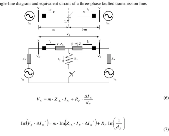
Considering the circuit in Fig. 1 and using the current distribution factor (dS) to represent the voltage drop over the fault resistance, the voltage equation at terminal X can be written as (6), where
RF represents the fault resistance. Multiplying both sides of (6) by the complex conjugate of ∆IX,
considering only the imaginary part, one can arrive at (7).
Fig. 1. Single-line diagram and equivalent circuit of a three-phase faulted transmission line.
S X F X L X d I R I Z m V 1 (6)
S F X X L X X d R I I Z m I V Im Im 1 Im 1 * * (7)If the system is considered homogeneous, the angle of dS will be approximately equal to zero. Thus, it can be considered that Im(1/dS) will be equal to zero. Then, isolating m in (7), one can arrive at (8), which represents the estimate of the fault location in percentage, according to the method proposed by [3].
100% Im Im * 1 * X X L X X I I Z I V m (8)It is noteworthy that this methodology is also known as the Takagi Method, which served as a basis for the formulation of many other techniques for fault location.
C MODIFIED TAKAGI METHOD (MTM)
This method is a modification of SIIFL. Proposed in [4], it considers the residual current (IR)
instead of the current variation at the time of the fault (ΔIX) in its formulation. In addition, it considers
a correction angle β, assumed to be equal to the source impedance angle. As a consequence of these considerations, the error due to the reactance effect is reduced. However, when considering β equal to the source impedance angle, the estimation of the fault location for single-phase short-circuits may
be inaccurate, since the ideal value of β to be adjusted varies for each point on the line. Eq. 9 represents the fault location estimated according to this method.
100% Im Im * 1 * j R X L j R X e I I Z e I V m (9) D NOVOSEL METHOD (NM)The method proposed in [8] calculates the distance to the fault point based on the distribution factor (dS), given by (10), and the post-fault voltage (VX) applied by the source in the line section
prior to the point at fault, according to (6).
L load X L load F S S Z Z Z Z m Z I I d 1 1 ) 1 ( (10)
In (10), ΔIX represents the variation of the source current in relation to the pre-fault and
post-fault periods, given by (5), and ZS, Zload and Z1L represent the source, load and line impedances,
respectively. Combining (10) and (6), it is possible to estimate the fault location, from a quadratic equation as a function of m, which is obtained by separating this equation in real and imaginary parts, as well as eliminating the fault resistance. Thus, the location of the fault will be given in per unit (p.u.). Substituting (10) in (6) and rearranging the terms, one can arrive at (11).
0 3 2 1 2 F R k k k m m (11)
Eq. 11 presents two unknown variables, being these m and RF. This equation can be separated
into real and imaginary parts. Eliminating RF in (11), the equation will have two roots. According to
[8], the appropriate solution for the distance to the fault is given by the root obtained according to (12), already in percentage in relation to the total length of the line.
% 100 2 4 2 N N N N N a c a b b m (12)
In (12), the parameters aN, bN and cN are given as a function of k1, k2 and k3. Further details on
the calculation of parameters k1, k2, k3, aN, bN, cN and RF can be found in [8].
Bretas and Salim Method
The method proposed in [11] uses data from one terminal and calculates the apparent impedance of a positive sequence up to the fault location. This method was proposed in order to
mitigate the effects of Distributed Generation (DG), since cogeneration and self-production modify systems that have only one flow, thus creating new sources of energy in the system. This technique estimates the fault point according to (13).
100% Im Im * 2 1 1 0 0 * X L L X X I I I Z I Z I V m (13)In (13), I0, I1 and I2 represent the zero, positive and negative sequence currents, taken from the
X terminal (Fig. 1). In addition, Z0L represents the zero-sequence impedance of the line.
3 METHODOLOGY AND TEST SYSTEM
Fig. 2 illustrates the test system implemented in the EMTP-ATP® software and used to obtain the voltage and current signals analysed in this study. Such system represents a TL with equivalent sources at both terminals, whose zero and positive sequence impedances are, respectively, ZS0 = 3.681
+ j24.515 and ZS1 = 0.819 + j7.757 Ω. The effective voltage value is 190 kV and the angle of SX is
delayed 30º in relation to the angle of SY. The TL has a total length of 100 km, with zero sequence
impedance equal to 0.1841 + j1.2258 Ω/km and positive sequence equal to 0.041 + j0.3878 Ω/km. The signals were measured at terminal X for different types of short-circuits and distances to the fault point (from 5 to 95% of the TL, with steps of 5%).
Fig. 2 Test system.
It is worth mentioning that all the FLs analysed were implemented in the Matlab® software. All the methods presented calculate the distance to the fault point from the moment of its detection until the breaker opening, given by the instant of actuation of the relay added to the time of extinction of the electric arc by the circuit breaker. The methods were evaluated in terms of the absolute error (eabs) of the fault location estimation, according to (14), as well as according to the distance estimated
at the time of the arc extinction, considering a circuit breaker with opening times of 4, 8 and 12 cycles, for sampling rates (N) of 8, 16, 32, 64 and 96 samples per cycle, for single-phase, phase-to-phase and three-phase faults at different points of the TL, without fault resistance. The phasors were obtained from a full cycle Fourier filter, without eliminating the DC component from the current signals.
r e abs m m
e (14)
In (14), me and mr represent the estimated position for the fault and the actual position of the
fault, respectively.
4 RESULTS AND DISCUSSIONS
In this Section, the conclusions about the transient behaviour of the responses of the analysed FLs are presented, as well as their performance in relation to the distance of the fault, the type of fault, the breaker opening time and the sampling rate are discussed.
A ANALYSIS OF THE TRANSIENT RESPONSE OF THE FLS
Among all the analysed cases, regarding the transient response of the methods, it was decided to detail the performance of the FLs for faults in 35%, 50% and 80% of the TL, for sampling rates of 32 and 64 samples per cycle, considering the breaker opening time equal to 8 cycles. The results for these cases are shown in Tabs. II to IV, where the best results are highlighted in bold. In general, it can be said that the high maximum error observed for the methodologies occurs during the first moments of estimation of the faulted point, what is due to the presence of the DC component in the current signals, which was not suppressed in this study. Therefore, it is worth mentioning that the use of methodologies for the removal of unidirectional components from fault currents should largely reduce the high values verified here.
TABLE III. RESULTS FOR THE PHASE-TO-PHASE FAULTS.
Observing the results in the Tabs. II to IV, it can be stated that, for single-phase faults and a sampling rate of 32 samples per cycle, none of the FLs was able to exceed the final value estimated by the distance relay. However, the SRM and BSM methods showed good precision in determining the faulted point with a final error between 100 and 300 m, since, in the case studied, each 1% represents 1 km of line. Similar results were obtained for sampling 64 samples per cycle, except for the fact that the best response was achieved by BSM for the single-phase fault in 80% of the LT.
Regarding phase-to-phase faults, it can be observed that the MTM presents better performance for short-circuits at 35 and 50% of the TL for both sampling rates. In 80% of the line, the best response was achieved by the SRM for 32 and 64 samples per cycle.
Finally, regarding three-phase faults, based on the data in the Tabs. II to IV, it is noted that the BSM presents better results in the two sampling rates for the short circuits in 35 and 50% of the TL, while the MTM and the SRM present the best final answer for faults in 80% in both sampling. It is also worth noting that the SIIFL and NM methods present the worst performance when estimating the distance from the faulted point at single-phase short-circuits. In addition, it is possible to observe that the error of the final estimate of the fault location increases for greater distances from the fault point in relation to the terminal where the voltage and current signals are measured for all FLs. This can best be seen in Figs. 3 to 5, which were obtained for a circuit breaker opening time equivalent to 4 cycles at 60 Hz at different sampling rates.
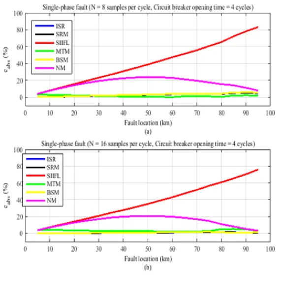
Analysing Figs. 3 and 4, it is possible to conclude that the response of the ISR, MTM and BSM FLs converges to the fault point in a few cycles for single-phase faults. For phase-to-phase faults, this also occurs for SIIFL, which, in single-phase faults, presents a greater error in estimating the fault location for greater distances.
Exclusively in relation to the performance of the NM for single-phase short-circuits, it should be noted that it presents better responses when faults occur near to the ends of the TL, increasing the estimation error as the faulted point approaches to the middle of the line, where the estimate error is maximum. However, for phase-to-phase faults, the error is considerably greater as the distance from the faulted point increases.
Based on the results presented in Fig. 5, one can conclude that, in general, for three-phase faults, the error in estimating the fault location also increases with its distance. It is important to note that behaviours similar to those presented in Figs. 3 to 5 are verified for the other opening times of the circuit breaker, since the estimation errors also increase with the same characteristics, except for the magnitude of the error, which decreases slightly, showing no significant improvement for longer opening times of the circuit breaker. Also, it is emphasized that the MTM performance improves a lot for three-phase faults with the increase of the circuit breaker opening time. These statements can
be better understood from Fig. 6, which shows the final average error of all cases analysed versus the breaker opening time, for each sampling rate used in this study.
B ANALYSIS OF THE PERFORMANCE OF FLS CONSIDERING THE SAMPLING RATE Based on the Figures in the previous section, it is possible to conclude that the response of the FLs improves with the increase of the sample rate. However, this improvement is significant for the SIIFL and NM methods (Fig. 6), which, even so, still have the highest average errors, regardless of the sampling rate and the opening time of the circuit breaker. For the other FLs, it can be said that the sampling rate does not significantly impact the response of the methodologies, since, for all sampling rates, their average errors show similar behaviours.
Fig. 3 Final absolute error of the response of the FLs versus the location of the single-phase fault for different sampling rates, and circuit breaker opening time equal to 4 cycles. a) N = 8 samples per cycle. b) N = 16 samples per cycle. c) N = 32 samples per cycle. d) N = 64 samples per cycle. e) N = 96 samples per cycle.
Fig. 4 Final absolute error of the response of the FLs versus the location of the phase-to-phase fault for different sampling rates, and circuit breaker opening time equal to 4 cycles. a) N = 8 samples per cycle. b) N = 16 samples per cycle. c) N = 32 samples per cycle. d) N = 64 samples per cycle. e) N = 96 samples per cycle.
Fig. 5 Final absolute error of the response of the FLs versus the location of the three-phase short-circuit for different sampling rates, and circuit breaker opening time equal to 4 cycles. a) N = 8 samples per cycle. b) N = 16 samples per cycle. c) N = 32 samples per cycle. d) N = 64 samples per cycle. e) N = 96 samples per cycle.
Fig. 6 Absolute average error of the response of the FLs versus circuit breaker opening time. a) N = 8 samples per cycle. b) N = 16 samples per cycle. c) N = 32 samples per cycle. d) N = 64 samples per cycle. e) N = 96 samples per cycle.
(a)
(c)
(d)
(e)
C ANALYSIS OF THE PERFORMANCE OF FLS CONSIDERING THE FAULT TYPE
Since the variation in the sampling rate does not significantly impact the performance of the methods, calculating the average error of the fault location estimation by the short-circuit type, it was possible to construct Fig. 7. From this Figure, one can see that, for any circuit breaker opening time, the SIIFL, NM and MTM methods present poor performances for the fault location in single-phase short-circuit situations. Also, it is noteworthy that SIIFL and MTM considerably improve their performance for phase-to-phase and three-phase faults, which is verified for NM only for three-phase
faults. For ISR, SRM and BSM methods the average error does not vary significantly in relation to the type of short-circuit, demonstrating that these methods are more robust and better perform the function of fault location, regardless of the type of fault, as well as the sampling rate and the circuit breaker opening time.
Fig. 7 Absolute average error of the response of the FLs versus fault type. a) Circuit breaker opening time of: a) 4 cycles; b) 8 cycles. c) 12 cycles.
5 CONCLUSIONS
The present work presents a study related to the behavior of the transient response of six methods aimed at locating faults based on the calculation of the impedance between the installation point and the faulted point, which is done based on data measured in one of the transmission line terminals. To this end, the FLs in question were tested for different types of faults, occurring at different points in the transmission line of a test system implemented in the ATPDraw, considering different circuit breaker opening times. From these tests it was possible to verify that the performances of the ISR, SRM and BSM methods are not significantly affected by the fault distance, as well as presenting good responses at different sampling rates, regardless of the breaker opening time. Regarding the SIIFL, MTM and NM methods, it can be said that their performance is affected by the parameters investigated here. In this context, it is stated that SIIFL and NM have the worst performances among the methodologies analyzed for single-phase and phase-to--phase faults, respectively, regardless of the sampling rate and the opening time of the circuit breaker, considerably improving their responses to three-phase faults. Finally, it is worth mentioning that, in future works, the same methodology used in this study will be applied to FLs presented recently, these being based on the calculation of impedance from data from one or more terminals, involving conditions not explored in this work, such as the influence of fault resistance, removal of the DC component, different angles of fault incidence and system loading.
REFERENCES
[1] T. Stringfield, D. Marihart, and R. Stevens, “Fault location methods for overhead lines”,
Transactions of the American Institute of Electrical Engineers. Part III: Power Apparatus and Systems, v. 76, p. 518-519, 1957.
[2] M. Sant and Y. Paithankar, “Online digital fault locator for overhead transmission line”, In: IET
Proceedings of the Institution of Electrical Engineers, v. 126, p. 1181-1185, 1979.
[3] T. Takagi et al., “Development of a new type fault locator using the one-terminal voltage and
current data”, IEEE Transactions on Power Apparatus and Systems, v. 101, p. 423-436, 1982.
[4] E. O. Schweitzer, “Evaluation and development of transmission line fault-locating techniques
which use sinusoidal steady-state information”, Computers & Electrical Engineering, v. 10, p. 269-278, 1983.
[5] L. Eriksson, M. M. Saha, and G. Rockefeller, “An accurate fault locator with compensation for
apparent reactance in the fault resistance resulting from remote-end infeed”, IEEE Transactions on Power Apparatus and Systems, v. 1, p. 423-436, 1985.
[6] K. Srinivasan and A. S. A. Jacques, “A new fault location algorithm for radial transmission lines
with loads”, IEEE Transactions on Power Delivery, v. 4, p. 1676-1682.
[7] D. Novosel et al., “Accurate fault location using digital relays”, In: Proceedings of the IICPST
Conference, p. 1120-1124, 1994.
[8] D. Novosel et al., “System for locating faults and estimating fault resistance in distribution
networks with tapped loads”, US Patent 5,839,093, 1998.
[9] M. Saha et al. “A new accurate fault locating algorithm for series compensated lines”, IEEE
Transactions on Power Delivery, v. 14, p. 789-797, 1999.
[10] A. Gopalakrishnan et al. “Fault location using the distributed parameter transmission line model”,
IEEE Transaction on Power Delivery, v. 15, p. 1169-1174, 2000.
[11] A. S. Bretas and R. H. Salim, “A new fault location technique for distribution feeders with
distributed generation”, WSEAS Transactions on Power Systems, WSEAS Press, v. 1, n. 5, p. 894, 2006.
[12] M. Farshad and J. Sadeh, "Accurate Single-Phase Fault-Location Method for Transmission Lines
Based on K-Nearest Neighbor Algorithm Using One-End Voltage," in IEEE Transactions on Power Delivery, vol. 27, no. 4, pp. 2360-2367, Oct. 2012.
[13] C. P. Reddy, D. V. S. S. S. Sarma and O. V. S. R. Varaprasad, "A novel fault classifier and locator
using one-end current spectrum and minimal synchronized symmetrical components for transmission lines," 2016 IEEE Annual India Conference (INDICON), Bangalore, pp. 1-6, 2016.
[14] S. S. Nagam, E. Koley and S. Ghosh, "Artificial Neural Network Based Fault Locator For Three
Phase Transmission Line with STATCOM," 2017 IEEE International Conference on Computational Intelligence and Computing Research (ICCIC), Coimbatore, pp. 1-4, 2017.
[15] IEEE Guide for determining fault location on ac transmission and distribution lines. IEEE Std