Essays in Applied Econometrics and Monetary
Policy
Essays in Applied Econometrics and Monetary Policy
A thesis submitted in fulfillment of the re-quirements for the degree of Doctor of Phi-losophy
EPGE FGV
Ficha catalográfica elaborada pela Biblioteca Mario Henrique Simonsen/FGV
Santos, Ana Flávia Soares dos
Essays in applied econometrics and monetary policy / Ana Flávia Soares dos Santos. - 2018.
121 f.
Tese (doutorado) - Fundação Getulio Vargas, Escola de Pós-Graduação em Economia.
Orientador: João Victor Issler. Inclui bibliografia.
1. Econometria. 2. Política monetária. I. Issler, João Victor. II. Fundação Getulio Vargas. Escola de Pós-Graduação em Economia. III. Título. CDD – 330.015195
I thank my family, who encouraged me and supported me unconditionally through-out my career.
Agradeço à minha família, que me incentivou e me apoiou incondicionalmente em toda a minha trajetória.
This thesis contains three independent chapters. The first one is about central bank credibility, where we measure people’s beliefs using survey data on inflation ex-pectations and focus on the 12-month-ahead horizon since it is widely used in the literature. Beliefs are measured by employing the panel-data setup of Gaglianone and Issler (2015), who show that optimal individual forecasts are an affine func-tion of one factor alone – the condifunc-tional expectafunc-tion of inflafunc-tion. This allows the identification and estimation of the common factor, our measure of people’s beliefs. Second, we compare beliefs with explicit (or tacit) targets by constructing Het-eroskedasticity and Autocorrelation Consistent (HAC) 95% asymptotic confidence intervals for our estimates of the conditional expectation of inflation, which is an original contribution of this paper. Whenever the target falls into this interval we consider the central bank credible. We consider it not credible otherwise. This ap-proach is applied to the issue of credibility of the Central Bank of Brazil (BCB) by using the now well-known Focus Survey of forecasts, kept by the BCB on infla-tion expectainfla-tions, from January 2007 until April 2017. Results show that the BCB was credible 65% of the time, with the exception of a few months in the begin-ning of 2007 and during the interval between mid-2013 throughout mid-2016. We also constructed a credibility index for this period and compared it with alternative measures of credibility.
In the second chapter, we show that it is possible to conciliate individual and consen-sus rationality tests, by developing a new framework to test for rational expectations hypothesis. We propose a methodology that verifies the consistency of the above mentioned expectation formation rule, where we explicitly allow for the possibility of heterogeneous expectations at the individual level, but also keeping individual and consensus expectations at the same system. We advance with respect to Keane and Runkle (1990)’s previous work, which argued that almost all existing tests in the literature so far were either incorrect or inadequate.
In the third chapter, we propose an individual coincident indicator for the following Latin American countries: Argentina, Brazil, Chile, Colombia and Mexico. In order to obtain similar series to those traditionally used in business-cycle research in constructing coincident indices (output, sales, income and employment) we back-cast several individual country series which were not available in a long time-series span. We also establish a chronology of recessions for these countries, covering the period from 1980 to 2012 on a monthly basis. Based on this chronology, the countries are compared in several respects. The final contribution is to propose an aggregate coincident indicator for the Latin American economy, which weights individual-country composite indices. Finally, this indicator is compared with the coincident indicator (The Conference Board – TCB) of the U.S. economy. We find that the U.S. indicator Granger-causes the Latin American indicator in statistical tests.
Figure 1 – Normal Distribution . . . 29
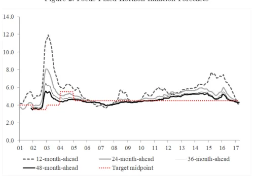
Figure 2 – Focus Fixed Horizon Inflation Forecasts . . . 31
Figure 3 – Forecasts vs Actual Inflation Rate for the 12-month-ahead horizon . . . 33
Figure 4 – Consensus Forecasts and Extended BCAF: 12-month-ahead horizon . . 35
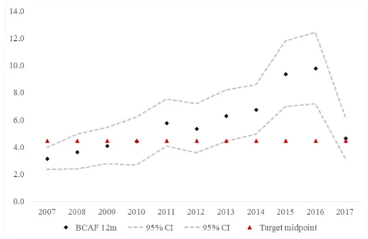
Figure 5 – BCAF and Confidence Intervals: 12-month-ahead . . . 36
Figure 6 – BCAF and Confidence Intervals vs. Inflation Target: Calendar Years. . 37
Figure 7 – Credibility Index . . . 37
Figure 8 – Comparison between Credibility Indexes proposed in the literature . . 38
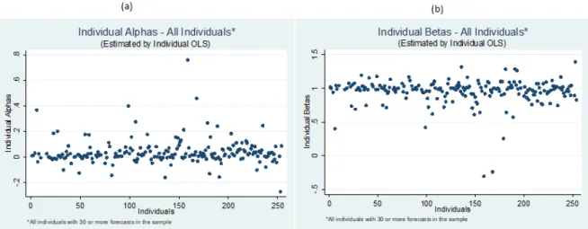
Figure 9 – Individual Alphas and Betas . . . 66
Figure 10 – Histogram of Individual Alphas and Betas . . . 67
Figure 11 – Argentina: Coincident Series . . . 83
Figure 12 – Brazil: Coincident Series . . . 84
Figure 13 – Chile: Coincident Series . . . 85
Figure 14 – Colombia: Coincident Series . . . 86
Figure 15 – Mexico: Coincident Series . . . 87
Figure 16 – Argentina: Coincident Indicator . . . 88
Figure 17 – Brazil: Coincident Indicator . . . 89
Figure 18 – Chile: Coincident Indicator. . . 89
Figure 19 – Colombia: Coincident Indicator . . . 90
Figure 20 – Mexico: Coincident Indicator . . . 91
Figure 21 – Latin America: Coincident Indicator . . . 92
Table 1 – Focus Inflation Forecasts: Descriptive Statistics* . . . 31
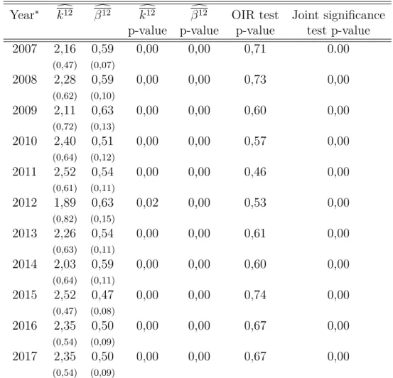
Table 2 – GMM estimation results for the 12-month-ahead forecast horizon . . . . 34
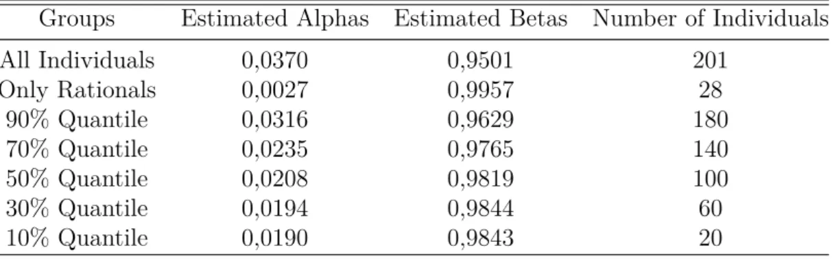
Table 3 – Average alphas and betas for selected groups . . . 67
Table 4 – Joint Hypothesis Tests on Coefficients: All Individuals* . . . 68
Table 5 – Joint Hypothesis Tests on Coefficients: Only Rational Individuals* . . . 68
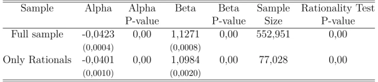
Table 6 – Results for Consensus Estimation . . . 69
Table 7 – Results for GMM Estimation: Original System vs. Modified System. . . 70
Table 8 – Tests P-values: Original System vs. Modified System . . . 71
Table 9 – Argentina: Turning Points . . . 88
Table 10 – Brazil: Turning Points . . . 88
Table 11 – Chile: Turning Points . . . 90
Table 12 – Colombia: Turning Points . . . 90
Table 13 – Mexico: Turning Points . . . 91
Table 14 – Harding and Pagan (2002)’s Concordance Index . . . 93
1 Central Bank Credibility and Inflation Expectations: A Microfounded
Fore-casting Approach . . . 10
1.1 Introduction . . . 11
1.2 The literature on central bank credibility . . . 13
1.3 Building a microfounded index. . . 19
1.3.1 Econometric Methodology . . . 19
1.3.2 Heteroskedasticity and autocorrelation consistent (HAC) covariance matrix estimation . . . 22
1.3.2.1 First case: 𝑁 → ∞ and then 𝑇 → ∞ . . . 24
1.3.2.2 Second case: 𝑇 → ∞ and 𝑁 is fixed or 𝑁 → ∞ after 𝑇 → ∞ 26 1.3.3 A new credibility index . . . 28
1.4 Empirical application . . . 29
1.4.1 Data . . . 29
1.4.2 Results . . . 33
1.4.3 Comparing with other indexes in the literature. . . 38
1.5 Conclusion . . . 39
2 A New Encompassing Model for Rationality Tests . . . 42
2.1 Introduction . . . 43
2.2 Inflationary expectations and rationality . . . 45
2.2.1 The Modeling of Expectations . . . 45
2.2.2 Rational Expectations Hypothesis: Empirical Evidence and Testing 47 2.3 Econometric Framework . . . 50
2.3.1 The Aggregation Problem . . . 50
2.3.2 A new encompassing framework for rationality tests . . . 53
2.3.3 GMM Estimation . . . 56 2.3.4 Hypothesis testing . . . 58 2.4 Empirical Application . . . 64 2.4.1 Data . . . 64 2.4.2 Stylized Facts . . . 65 2.4.3 GMM Estimation Results . . . 69 2.5 Conclusion . . . 71
3 Constructing Coincident Indices of Economic Activity for the Latin Ameri-can Economy . . . 73
3.2 Literature Review . . . 75
3.2.1 International Experience . . . 75
3.2.2 Latin America Experience . . . 77
3.3 Theoretical underpinnings . . . 78
3.3.1 The Methodology of TCB . . . 78
3.3.2 Back-casting . . . 79
3.4 Empirical Results . . . 81
3.4.1 The Coincident Series . . . 81
3.4.1.1 Argentina . . . 82
3.4.1.2 Brazil . . . 83
3.4.1.3 Chile. . . 84
3.4.1.4 Colombia . . . 85
3.4.1.5 Mexico . . . 86
3.5 The coincident indicator . . . 87
3.5.1 Argentina . . . 87 3.5.2 Brazil . . . 87 3.5.2.1 Chile. . . 89 3.5.3 Colombia . . . 89 3.5.4 Mexico . . . 90 3.5.5 Latin America . . . 91 3.6 Conclusion . . . 93 Bibliography . . . 95
Appendix
108
APPENDIX A Technical Appendix . . . 109APPENDIX B Assumptions and Propositions of Gaglianone and Issler (2015)113 APPENDIX C Additional Tables . . . 118
1 Central Bank Credibility and Inflation
Ex-pectations: A Microfounded Forecasting
Approach
Abstract
Credibility is elusive and no generally agreed upon measure of it exists. Despite that, as argued by Blinder (2000), there is a consensus that "A central bank is credible if
people believe it will do what it says". This paper proposes a measure of credibility
based upon this definition. A main challenge is that, to implement it, one needs a measure of people’s beliefs and of what central banks say they do in the first place. Even possessing these two, one later needs a way to compare whether they are the same or not. We approach this problem in a novel way. To keep it tractable, we focus on inflation expectations, since inflation is arguably the main variable central banks care about.
Our approach is as follows. First, we measure people’s beliefs using survey data on inflation expectations. We focus on the 12-month ahead horizon since it is widely used in the literature. Beliefs are measured by employing the panel-data setup of Gaglianone and Issler (2015), who show that optimal individual forecasts are an affine function of one factor alone – the conditional expectation of inflation. This al-lows the identification and estimation of the common factor, our measure of people’s beliefs. Second, we compare beliefs with explicit (or tacit) targets by constructing Heteroskedasticity and Autocorrelation Consistent (HAC) 95% asymptotic confi-dence intervals for our estimates of the conditional expectation of inflation, which is an original contribution of this paper. Whenever the target falls into this interval we consider the central bank credible. We consider it not credible otherwise. This approach is applied to the issue of credibility of the Central Bank of Brazil (BCB) by using the now well-known Focus Survey of forecasts, kept by the BCB on infla-tion expectainfla-tions, from January 2007 until April 2017. Results show that the BCB was credible 65% of the time, with the exception of a few months in the begin-ning of 2007 and during the interval between mid-2013 throughout mid-2016. We also constructed a credibility index for this period and compared it with alternative measures of credibility.
Key words: Consensus Forecasts, Forecast Combination, Panel Data, Central Banking.
1.1
Introduction
Over the last four decades, the question of central bank credibility has been ex-tensively studied by the academic literature on monetary policy. It has also become a major concern for many central bankers around the world, which have taken a number of measures to enhance the credibility of monetary policy. Building central bank credibility was especially strong in countries under Inflation Targeting regimes, given the role that expectations have in most economic models incorporating them, where it serves as a way of anchoring inflation expectations by clearly stating the target and communicating its intentions on how to to steer actual inflation toward that target.
A main problem is that credibility is elusive and no generally agreed upon measure of it exists. For example, Blinder (2000) states, "A central bank is credible if people believe it will do what it says." It is very hard to argue against such a definition of credibility, being the reason why it became so popular among central bankers and academics alike.
This paper proposes a measure of credibility that is based upon this definition. A main challenge is that, to implement it, one needs a measure of people’s beliefs and of what central banks say they do in the first place. Even possessing these two, one later needs a way to compare whether they are the same or not. We approach this problem in a novel way. To keep it tractable, we focus on inflation expectations, since inflation is arguably the main variable central banks care about. Indeed, many countries are users of Inflation Targeting with explicit targets (Brazil included), but, even if they are not, there is usually a tacit agreement on what that target should be at different points in time.
Our approach is as follows. First, we measure people’s beliefs using survey data on inflation’s expectations1. This is done by employing the panel-data setup of Gaglianone
and Issler(2015). They show that optimal individual forecasts are an affine function of one factor alone – the conditional expectation of inflation. In this setup, individual forecasts can be a bias ridden version of the conditional expectation of inflation if individuals have no knowledge of the true DGP of inflation, if they possess an asymmetric loss function, or both. Although this is true for individuals, we assume that markets operate under a mean-squared-error risk function with knowledge of inflation’s DGP. Therefore, people’s beliefs will be equal to the conditional expectation of inflation, since this function minimizes the loss functions for the market as a whole. This allows the identification and estimation of our measure of people’s beliefs. Second, we compare beliefs with explicit (or tacit) targets. Therefore, our measure of what central banks say they do are these targets, which serve as a binding contract between central banks and society. To compare people’s beliefs with what central banks say they do, we need to take into account the fact that our estimate of people’s beliefs are measured with uncertainty, which is true for any estimate including
1 We focus on 12-month-ahead horizon since it is widely used in the literature and it is the most
ours. Thus, we construct Heteroskedasticity and Autocorrelation Consistent (HAC) 95% asymptotic confidence intervals for our estimates of the conditional expectation of infla-tion. Whenever the target falls into this interval we consider the central bank credible. We consider it not credible otherwise.
Of course, there has been active research in the area of credibility, especially in this millennium. Regarding measurement, a pioneering work is due to Svensson (1993), who proposed a simple test to check whether the inflation target is credible in the sense that market agents believe that future inflation will fall within the target range. A number of articles followed, trying to construct credibility measures and indices in the last two decades; see Bomfim and Rudebusch (2000), Cecchetti and Krause (2002), Mendonça and Souza (2007,2009), Levieuge at al. (2016), Bordo and Siklos (2015), inter alia. We advance with respect to this literature in three ways: (i) as we discuss below, in most of these papers people’s beliefs are not correctly specified or estimated. Here, we just need panel-data on inflation expectations to estimate consistently beliefs; (ii) most of these papers adopt ad hoc confidence bands in making comparisons between beliefs and targets. This creates a problem of measurement. Even if these confidence bands are appropriate for a given country in a specific point in time, they may not be appropriate for a different country and/or on a different point in time for the same country; (iii) the application of our approach is straightforward for countries under an inflation targeting program. However, it extends naturally to other countries in which a tacit target is present.
The approach discussed above is applied to study the credibility of the Central Bank of Brazil (BCB) by using the now well-known Focus Survey of forecasts, kept by the BCB on inflation expectations. This is a world-class database, fed by institutions that include commercial banks, asset management firms, consulting firms, non-financial institutions, etc. About 250 participants can provide daily forecasts for a large number of economic variables, e.g., inflation using different price indices, interest and exchange rates, GDP, industrial production, etc., and for different forecast horizons, e.g., current month, next month, current year, 5 years ahead, among others. At any point in time, about 100 participants are active using the system that manages the database. The survey has several key features: (i) participants can access the survey at any time and we can observe their decisions to update or not their forecasts; (ii) the confidentiality of information is guaranteed and the anonymity of forecasters is preserved, i.e., there are no reputational concerns; (iii) the Focus Survey has very strong incentives for participants to update their forecasts, specially on inflation expectations; see Carvalho and Minella (2012) and Marques (2013) for further details. To apply the techniques discussed above on the Focus Survey, we first extend the work of Gaglianone and Issler (2015) by deriving a robust HAC estimator for the asymptotic variance of the inflation expectation estimator proposed there. This is an additional original contribution of this paper.
Based on this framework, the asymptotic variance of the inflation expectation is obtained on a monthly basis for the Focus Survey database, together with the conditional expectation of inflation 12-months ahead, constructing the 95% HAC confidence intervals for inflation expectations from January 2007 until April 2017. This is compared to the target in the Brazilian Inflation Target Regime. Results show that the BCB was credible 65% of the time, with the exception of a few months in the beginning of 2007 and during the interval between mid-2013 throughout mid-2016. We also constructed a credibility index for this period and compared it with alternative measures of credibility previously developed in the literature.
The remainder of this paper is organized as follows. Section 1.2 discusses the existing literature on central bank credibility and brings a discussion about the existing indexes. Section1.3gives an informal overview of the main results of Gaglianone and Issler (2015), a step-by-step description of the HAC covariance matrix estimation procedure and develops a new credibility index for the central bank based on this measure. Section 1.4 brings an empirical application of this framework to evaluate the credibility of the BCB in recent years, using the Focus Survey database. Section 1.5 concludes.
1.2
The literature on central bank credibility
The issue of whether it is better for the policymaker to operate with pure discre-tion and poor accountability or to commit to a policy has long been a central quesdiscre-tion for monetary policy. Kydland and Prescott (1977) showed that a regime where policy-makers have to precommit to behave in a particular way is preferable to a regime that allows policymakers to choose a different policy at each point in time, because agents re-optimize dynamically. The main idea behind the dynamic optimization argument is that expectations play a central role in macroeconomic dynamics, a concept that was first emphasized by Muth (1961)’s theory of rational expectations and later by Friedman (1968) and Phelps (1967, 1968), gaining further attention with the the earliest rational expectations models of Lucas (1972, 1973) and Sargent and Wallace (1975).
Several central banks have adopted a more systematic approach to maintain price stability in the early 90s, particularly with an inflation targeting as a method of com-mitment, explicitly acknowledging that low and stable inflation is the overriding goal of monetary policy and retaining "constrained discretion", as argued by Bernanke and Mishkin (1997). At the same time, the theoretical debate in favor of monetary policy rules gained traction with Taylor (1993).
The evolution and the improvement of the monetary policy institutional framework are related in many empirical studies to better economic outcomes. It is widely agreed2 2 See Alesina (1988), Alesina and Summers (1993), Cukierman (2008), Cukierman et al. (1992), Grilli
that independent, transparent, accountable and credible central banks are able to deliver better policy outcomes. Cecchetti and Krause (2002) study a large sample of countries and find that credibility is the primary factor explaining the cross-country variation in macroeconomic outcomes. Taylor (2000) and Carrière-Swallow et al. (2016) find evidence that price stability and greater monetary policy credibility create an endogenous reduc-tion in the pass-through to consumer prices. More recently, central banks are certainly more transparent than anytime in history and many communications practices have been used to better align public’s expectations and the objectives of monetary policy, forward guidance3 is communicated and, in some cases, future interest rate path is published4,5.
The agents’ expectations regarding central bank policy is directly tied to the con-cept of credibility. Cukierman (1986) define monetary policy credibility as "the absolute value of the difference between the policy-maker’s plans and the public’s beliefs about those plans". In our view, a less controversial and cleaner definition is given by Blinder (1999), who argues that "a central bank is credible if people believe it will do what it says". Re-gardless of the definition, central bank credibility in the literature is usually related to a reputation6 built based on strong aversion to inflation7 or a framework that is
character-ized by an explicit contract with incentive compatibility8 or a commitment to a rule or a
specific and clear objective.
Svensson (1993) was the first to propose a test to monetary policy credibility, in the sense that market agents believe that future inflation will be on the target. Following Cukierman and Meltzer (1986)’s definition of credibility, related to the absolute value between public’s expectations and the policymaker’s plans, he proposes to compare ex-post target-consistent real interest rates with market real yields on bonds. If market rates fall outside the range, credibility in expectations can be rejected. In the case where the central bank has an explicit inflation target, Svensson (2000) proposes to measure credibility as the distance between the expected inflation and the target.
Bomfim and Rudebusch (2000) suggest another approach, measuring overall cred-ibility by the extent to which the announcement of a target is believed by the private
et al. (1991), Rogoff (1985), among others
3 The FOMC statement on March, 2009, introduced the forward guidance language in the monetary
policy toolkit.
4 The Norges Bank, The Swedish Riksbank and the Reserve Bank of New Zealand publish in their
quarterly monetary policy report the expected path for policy rates.
5 Bomfim and Rudebusch (2008) show that central bank communication of interest rate projections
can help shape financial market expectations and may improve macroeconomic performance.
6 Rogoff (1985) suggested that monetary policy should be placed in the hands of an independent central
bank run by a ’conservative’ central banker who would have a greater aversion to inflation than that of the public at large. This would help to reduce the inflation bias inherent in discretion.
7 More recently, after the 2008 financial crisis, central bank credibility has also been very much tied to
strong aversion to deflation in many advanced economies.
8 Canzoneri (1985), Persson (1993) and Walsh (1995) have analyzed alternative ways of allowing
sector when forming their long-run inflation expectations. Specifically, they assume that the expectation of inflation at time 𝑡, denoted 𝜋𝑒
𝑡, is a weighted average of the current
target, denoted by 𝜋𝑡, and last period’s (12-months) inflation rate, denoted by 𝜋𝑡−1:
𝜋𝑒𝑡 = 𝜆𝑡𝜋𝑡+ (1 − 𝜆𝑡)𝜋𝑡−1
The parameter 𝜆𝑡, with (0 < 𝜆𝑡< 1) indexes the credibility of the central bank. If 𝜆𝑡= 1,
there is perfect credibility, and private sector’s long-run inflation expectations will be equal to the announced long-run goal of the policymaker. If 𝜆𝑡= 0, there is no credibility,
and the inflation target is ignored in the formation of expectations. Intermediate values of 𝜆𝑡 represent partial credibility of the announced ultimate inflation target.
Following Bomfim and Rudebusch (2000), Demertzis et al. (2008) model inflation and inflation expectations in a general VAR framework, based on the fact that the two variables are intrinsically related. When the level of credibility is low, inflation will not reach its target because expectations will drive it away, and expectations themselves will not be anchored at the level the central bank wishes. They apply their framework to a group of developed countries and compute an "anchoring effect" based on 𝜆𝑡.
Cukierman and Meltzer (1986)’s approach was also further explored in the lit-erature after Svensson’s work, and a number of articles proposed different criteria for measuring central bank credibility. The preferred measure is the average 12-month-ahead inflation expectations from surveys with private agents (consumers and/or professional forecasters) but they differ in the way that they define how fast the credibility decays, which thresholds to choose, whether to penalize or not negative deviations (expectations below actual inflation) and the symmetry of the index.
Cecchetti and Krause (2002) construct an index of policy credibility that is an inverse function of the gap between expected inflation and the central bank’s target level, taking values from 0 (no credibility) to 1 (full credibility). The index is defined as follows:
𝐼𝐶𝐾 = ⎧ ⎪ ⎪ ⎪ ⎪ ⎨ ⎪ ⎪ ⎪ ⎪ ⎩ 1 if 𝜋𝑒 ≤ 𝜋 𝑡 1 − 𝜋𝑒−𝜋𝑡 20%−𝜋𝑡 if 𝜋𝑡≤ 𝜋 𝑒≤ 20% 0 if 𝜋𝑒 ≥ 20%
where 𝜋𝑒 is the expected inflation and 𝜋
𝑡 is the central bank target. Between 0 and 1 the
value of the index decreases linearly as expected inflation increases. The authors define 20% as an ad hoc upper bound, which is questionable and certainly changes from one economy to another. Many central banks that have maintained low and stable inflation for decades would consider a much lower bound. Besides that, after the 2008 financial crisis, many central banks have been more worried about deflation risks, and the index
proposed by Cecchetti and Krause (2002) considers only positive deviations as a factor relevant for credibility loss.
Mendonça and Souza (2007, 2009) propose an extension to Cecchetti and Krause (2002)’s index considering that not only positive deviations but also negative deviations of inflation expectations from the target can generate a loss of credibility9. The index
proposed by the latter is:
𝐼𝐷𝑀 𝐺𝑆 = ⎧ ⎪ ⎪ ⎪ ⎪ ⎪ ⎪ ⎪ ⎪ ⎨ ⎪ ⎪ ⎪ ⎪ ⎪ ⎪ ⎪ ⎪ ⎩ 1 if 𝜋𝑚𝑖𝑛 𝑡 ≤ 𝜋𝑒 ≤ 𝜋𝑚𝑎𝑥𝑡 1 − 𝜋𝑒−𝜋𝑚𝑎𝑥𝑡 20%−𝜋𝑚𝑎𝑥𝑡 if 𝜋 𝑚𝑎𝑥 𝑡 < 𝜋𝑒 < 20% 1 −𝜋𝑒−𝜋𝑚𝑖𝑛𝑡 −𝜋𝑚𝑖𝑛 𝑡 if 0 < 𝜋𝑒 < 𝜋 0 if 𝜋𝑒 ≥ 20% or 𝜋𝑒≤ 0
where 𝜋𝑒 is the inflation expectation of the private sector and 𝜋𝑚𝑖𝑛
𝑡 and 𝜋𝑚𝑎𝑥𝑡 represent
the lower and upper bounds of the inflation target range, respectively. The central bank is viewed as non credible (𝐼𝐷𝑀 𝐺𝑆 = 0) if expected inflation is equal or greater than 20%
or lower than or equal to 0%. The two indexes above consider that outside certain ranges, credibility is zero.
Levieuge et al. (2016) believe that negative deviations of inflation expectations from the target are less likely to compromise credibility than positive deviations. They provide an asymmetric measure of credibility based on the linear exponential (LINEX) function, as follows:
𝐼𝐿 = 𝑒𝑥𝑝(𝜑(𝜋𝑒−𝜋))−𝜑(𝜋1 𝑒−𝜋), for all 𝜋𝑒
where 𝜋𝑒 is the inflation expectations of the private sector, 𝜋 is the inflation target and, for 𝜑 = 1, positive deviations (𝜋𝑒 > 𝜋) will be considered more serious than negative deviations (𝜋𝑒 < 𝜋) as the exponential part of the function dominates the linear part
when the argument is positive. As the previous indexes, when 𝐼𝐿 = 1 the central bank
has full credibility and when 𝐼𝐿= 0 there is no credibility at all.
Bordo and Siklos (2015) propose a comprehensive approach to find cross-country common determinants of credibility. They organize sources of changes in credibility into groups of variables that represent real, financial, and institutional determinants for the proposed central bank credibility proxy. Their preferred definition of central bank credi-bility is written as follows:
9 Mendonça and Souza (2007) considers that perfect credibility occurs when inflation expectations are
exactly in the target midpoint, and it decreases linearly until the upper and lower bounds of the target range and Mendonça and Souza (2009) considered a target range instead of a target point.
𝐼𝐵𝑆 = ⎧ ⎪ ⎨ ⎪ ⎩ 𝜋𝑒𝑡+1− 𝜋𝑡 if 𝜋𝑡− 1 ≤ 𝜋𝑡+1𝑒 ≤ 𝜋𝑡+ 1 (𝜋𝑒 𝑡+1− 𝜋𝑡)2 if 𝜋𝑡− 1 > 𝜋𝑒𝑡+1> 𝜋𝑡+ 1 where 𝜋𝑒
𝑡+1 is the one-year-ahead inflation expectations and 𝜋𝑡is the central bank target.
Credibility is then defined such that the penalty for missing the target is greater when expectations are outside the 1% interval than when forecasts miss the target inside this 1% range.
There is also a strand of literature that apply state space models and the Kalman Filter to develop credibility measures, since it is a latent variable; see Hardouvelis and Barnhart (1989) and Demertzis et al. (2012). In a recent contribution, Vereda et al. (2017) apply this framework to the term structure of inflation expectations in Brazil to estimate the long-term inflation trend, as it can be associated to the market perception about the target pursued by the central bank. They follow Kozicki and Tinsley (2012)’s methodology and treat the so called shifting inflation endpoint as a latent variable estimated using the Kalman filter. The disagreement between forecasters is also related to a credibility measure, focusing not on the consensus forecast, but also on the distribution of the cross-section of forecasts; see Dovern, Fritsche and Slacalek (2012) and Capistrán and Ramos-Francia (2010).
Finally, Garcia and Lowenkron (2007) and Garcia and Guillén (2014) also bring relevant contributions to the brazilian literature. Garcia and Lowenkron (2007) study the relation between agents’ inflation expectations 12 months ahead and inflation surprises and also look at inflation-linked bonds to evaluate the relation with inflation risk premia. Garcia and Guillén (2014) look at the distribution of inflation expectations using a Markov chain approach, based on the fact that if an agent is persistently optimistic or pessimistic about inflation prospects10, this implicitly reveal a bias, which is an evidence of lack of credibility.
As we can see, the literature that tried to measure central bank credibility fo-cused on measures that involve private sector expectations of inflation. In that sense, it is natural to ask if such expectations are reasonably measured or, in other words, reflect private expectations free of bias. It is well known that, under a mean-squared-error risk function, the optimal forecast is the conditional expectation. However, individual agents or professional forecasters may have an asymmetric loss function for a variety of reasons11.
So, the answer to this question is no.
The direct measures of inflation expectations involve surveys with professional forecasters, consumers or firms, while indirect measures are market expectations implied in
10 The concept of optimistic or pessimistic here is related to an inflation forecast that is below or above
the inflation target, respectively.
bond prices. King (1995) argues in favor of indirect measures, such as market expectations implied in bond prices, because they are available at higher frequency. However, there is a literature on inflation forecasting that argues that survey based methods outperform a number of model based forecasts12and, besides that, in the Brazilian case the availability of daily forecasts from professional forecasters at the Focus Survey database provides rich information about direct measures on inflation expectations.
The great majority of the indexes described above use average 12-month-ahead inflation expectations from surveys. But, as we will argue, survey-based forecasts can be biased, and there are many sources of forecast bias. Forecasters may have economic incentives to make biased forecasts and may also have asymmetric loss functions over forecast errors. Besides that, there is influence of information rigidities in the formation of inflation expectations, which is also a potential source of bias. Previous research13 has
shown that in the particular case of Brazil, professional forecasters are biased, as they persistently overestimate or underestimate inflation.
Not only there is evidence that the consensus expectations is an imperfect measure, but also there are other critics to the existing indexes. The measures that relates inflation expectations to the target usually need a threshold14, above/under which the credibility
is null. But in all cases previously discussed, this threshold is ad hoc and cannot be generalized to all countries. As it reduces the validity and the comparability of the index between countries and also between years for the same country, we think a threshold based on a statistical criteria is better, such that it could be generalized among countries and compared over time.
There is also a discussion about whether credibility is linear or not, and if it is symmetric or not. Certainly credibility is not linear15, and that is why we think that an
index can be better analyzed if it is presented with a confidence region. Credibility is related with agents’ perceptions, therefore it is very simplistic to try to resume a very complex relation in one number and a more comprehensive measure can be obtained through an interval.
Now that we discussed the ideal features that a credibility analysis should have, we show in more details the econometric methodology in the next section and the setup behind our index.
12 Ang et al. (2007) argue that methods that employ true out-of-sample survey-based forecasts
pro-vided by economic agents (consumers and/or professional forecasters) outperform a large number of out-of-sample single-equation and multivariate time-series models, even comparing with information embedded in asset prices. This is consistent with Faust and Wright (2013)’s argument that subjective forecasts of inflation seem to outperform model-based forecasts.
13 See Garcia and Guillén (2014)
14 Cecchetti and Krause (2002) and Mendonça and Souza (2007, 2009) set credibility equal to zero
below/above a certain ad hoc threshold.
1.3
Building a microfounded index
This section brings a discussion of the econometric methodology proposed by Gaglianone and Issler (2015)16 to combine survey expectations17 in order to obtain
opti-mal forecasts in a panel-data context. Their main assumptions and propositions are listed on Appendix B with more detail. The techniques to obtain the bias corrected average forecast (BCAF) are explained and we further discuss how to obtain the asymptotic dis-tribution of this estimator, using heteroskedasticity and autocorrelation consistent (HAC) covariance matrix estimation methods.
1.3.1
Econometric Methodology
The techniques proposed by Gaglianone and Issler (2015) are appropriate for fore-casting a weakly stationary and ergodic univariate process {𝑦𝑡} using a large number of
forecasts that will be combined to yield an optimal forecast in the mean-squared error (MSE) sense. The forecasts for 𝑦𝑡 are taken from a survey of agents’ expectations
regard-ing the variable in question and are computed usregard-ing conditionregard-ing information sets lagged ℎ periods. These ℎ-step-ahead forecasts of 𝑦𝑡 formed at period (𝑡 − ℎ) are labeled 𝑓𝑖,𝑡ℎ, for
𝑖 = 1, ..., 𝑁 , 𝑡 = 1, ..., 𝑇 and ℎ = 1, ..., 𝐻, where 𝑁 is the number of respondents of an opinion poll regarding 𝑦𝑡.
The econometric setup includes two layers, where in the first layer the individual form his optimal point forecast of 𝑦𝑡 (𝑓𝑖,𝑡ℎ) and in the second layer the econometrician
uses the information about individual forecasts to make inference about the conditional expectation E𝑡−ℎ(𝑦𝑡). They show that optimal forecasts, are related to the conditional
expectation E𝑡−ℎ(𝑦𝑡) by an affine function:
𝑓𝑖,𝑡ℎ = 𝑘𝑖ℎ+ 𝛽𝑖ℎ· E𝑡−ℎ(𝑦𝑡) + 𝜀ℎ𝑖,𝑡 (1.1)
This is the optimal ℎ-step-ahead feasible forecast of 𝑦𝑡 for each forecaster 𝑖 in the
sample, where 𝜃ℎ𝑖 = [𝛽𝑖ℎ 𝑘ℎ𝑖]′ is a (2 × 1) vector of parameters and 𝜀ℎ𝑖,𝑡 accounts for finite sample parameter uncertainty. As we do not need identification of all 𝛽𝑖ℎ and 𝑘𝑖ℎ, to be able to identify E𝑡−ℎ(𝑦𝑡), the only focus is on their means. Then, averaging across 𝑖 and
assuming that 1 𝑁 ∑︀𝑁 𝑖=1𝜀ℎ𝑖,𝑡 𝑝 −
→ 0, allows identifying E𝑡−ℎ(𝑦𝑡) as:
E𝑡−ℎ(𝑦𝑡) = 𝑝𝑙𝑖𝑚𝑁 →∞ 1 𝑁 ∑︀𝑁 𝑖=1𝑓𝑖,𝑡ℎ − 𝑁1 ∑︀𝑁 𝑖=1𝑘𝑖ℎ 1 𝑁 ∑︀𝑁 𝑖=1𝛽𝑖ℎ (1.2)
16 It should be mentioned that this methodology extends the previous literature of forecasting in a
panel-data context (see Palm and Zellner (1992), Davies and Lahiri (1995), Issler and Lima (2009), Lahiri, Peng and Sheng (2015).
under the assumption that the terms of the limit above converge in probability.
The basic idea is to estimate the random variable E𝑡−ℎ(𝑦𝑡) through GMM
tech-niques relying on 𝑇 asymptotics. But as the loss function is known only by the individual forecaster, and this is an important source of heterogeneity in the forecasts, 𝑓ℎ
𝑖,𝑡 is a bias
and error ridden conditional expectation. Issler and Lima (2009) proposed to decompose 𝑦𝑡 such that:
𝑦𝑡= E𝑡−ℎ(𝑦𝑡) − 𝜂𝑡ℎ (1.3)
where 𝜂ℎ
𝑡 is a martingale-difference sequence and, by construction, E𝑡−ℎ(𝜂𝑡ℎ) = 0.
There-fore, they can use this decomposition to express 𝑓ℎ
𝑖,𝑡 in the following way:
𝑓𝑖,𝑡ℎ = 𝑘ℎ𝑖 + 𝛽𝑖ℎ· 𝑦𝑡+ 𝜈𝑖,𝑡ℎ (1.4)
where 𝜈𝑖,𝑡ℎ ≡ 𝛽ℎ
𝑖·𝜂ℎ𝑡+𝜀ℎ𝑖,𝑡is a composite error term. Under the assumption that E(𝜈𝑖,𝑡ℎ|ℱ𝑡−ℎ) =
018, where ℱ
𝑡−ℎ is the information set available at 𝑡 − ℎ, it follows that:
E[𝜈𝑖,𝑡ℎ ⊗ 𝑧𝑡−𝑠] = E[(𝑓𝑖,𝑡ℎ − 𝑘𝑖ℎ− 𝛽𝑖ℎ· 𝑦𝑡) ⊗ 𝑧𝑡−𝑠] = 0 (1.5)
for all 𝑖 = 1, ..., 𝑁 , 𝑡 = 1, ..., 𝑇 and all ℎ = 1, ..., 𝐻, and where 𝑧𝑡−𝑠 is a vector of
instru-ments, 𝑧𝑡−𝑠 ∈ ℱ𝑡−𝑠 with 𝑠 = ℎ and ⊗ is the Kronecker product. But, as this moment
conditions have too many parameters and as the parameters to be estimated by GMM don’t depend on 𝑖, they use cross-section averages to reduce parameter dimensionality, as long as there is convergence in probability, leading to:
E[(𝑓.,𝑡ℎ − 𝑘ℎ− 𝛽ℎ· 𝑦𝑡) ⊗ 𝑧𝑡−𝑠] = 0 (1.6)
for all 𝑡 = 1, ..., 𝑇 and ℎ = 1, ..., 𝐻 and where 𝑓ℎ .,𝑡 = 𝑁1 ∑︀𝑁 𝑖=1𝑓𝑖,𝑡ℎ, 𝑘ℎ = 1 𝑁 ∑︀𝑁 𝑖=1𝑘𝑖ℎ, and 𝛽ℎ = 1 𝑁 ∑︀𝑁
𝑖=1𝛽𝑖ℎ. Therefore, to be able to identify and estimate E𝑡−ℎ(𝑦𝑡) from a survey of
forecasts, since E𝑡−ℎ(𝑦𝑡) does not vary across 𝑖, averaging across 𝑖 is a good strategy.
If we stack all moment conditions implicit in equation1.6 across ℎ, it is even more clear that the initial problem collapsed to one where we have 𝐻 × 𝑑𝑖𝑚(𝑧𝑡−𝑠) restrictions
and 2𝐻 parameters to estimate19: 18
As we noted before, by construction, E(𝜂𝑡ℎ|ℱ𝑡−ℎ) = 0, so the assumption needed to obtain
E(𝜈𝑖,𝑡ℎ |ℱ𝑡−ℎ) = 0 is only that E(𝜀ℎ𝑖,𝑡|ℱ𝑡−ℎ) = 0.
19 We should remember that over-identification requires that 𝑑𝑖𝑚(𝑧
E ⎡ ⎢ ⎢ ⎢ ⎢ ⎢ ⎢ ⎣ (𝑓1 .,𝑡− 𝑘1− 𝛽1 · 𝑦𝑡) (𝑓2 .,𝑡− 𝑘2− 𝛽2 · 𝑦𝑡) ... (𝑓𝐻 .,𝑡 − 𝑘𝐻 − 𝛽𝐻 · 𝑦𝑡) ⎤ ⎥ ⎥ ⎥ ⎥ ⎥ ⎥ ⎦ ⊗ 𝑧𝑡−𝑠 = 0
There are two cases here, regarding the limit in equation (1.2). The first case is when we let first 𝑁 → ∞ and then we let 𝑇 → ∞. The second is when we first let 𝑇 → ∞ and 𝑁 is fixed or 𝑁 → ∞ after 𝑇 .
In the first case, note that under suitable conditions, the cross-sectional aver-ages in (1.6) would converge in probability to a unique limit as 𝑁 → ∞, that is, 𝑝𝑙𝑖𝑚𝑁 →∞𝑁1 ∑︀𝑁𝑖=1𝛽𝑖ℎ = 𝛽ℎ, 𝛽ℎ ̸= 0 and |𝛽ℎ| < ∞; 𝑝𝑙𝑖𝑚𝑁 →∞𝑁1 ∑︀𝑁𝑖=1𝑘ℎ𝑖 = 𝑘ℎ, 𝑘ℎ ̸= 0
and |𝑘ℎ| < ∞ and 𝑝𝑙𝑖𝑚
𝑁 →∞𝑁1 ∑︀𝑁𝑖=1𝑓𝑖,𝑡ℎ = 𝑓.,𝑡ℎ, 𝑓.,𝑡ℎ ̸= 0 and |𝑓.,𝑡ℎ| < ∞, for all 𝑡 = 1, ..., 𝑇 .
After taking moment conditions and noting that 𝑁 → ∞:
E[𝜈𝑖,𝑡ℎ ⊗ 𝑧𝑡−𝑠] = E[(𝑓𝑖,𝑡ℎ − 𝑘 ℎ 𝑖 − 𝛽
ℎ
𝑖 · 𝑦𝑡) ⊗ 𝑧𝑡−𝑠] = 0 (1.7)
They show20that the feasible extended bias corrected forecast 1
𝑁 ∑︀𝑁 𝑖=1 𝑓ℎ 𝑖,𝑡−𝑘̂︀ℎ ̂︁ 𝛽ℎ , based
on 𝑇 -consistent GMM estimates 𝜃̂︁ℎ = [𝑘̂︁ℎ;𝛽̂︁ℎ]′ obeys the following condition:
E𝑡−ℎ(𝑦𝑡) = 𝑝𝑙𝑖𝑚(𝑁,𝑇 →∞)𝑠𝑒𝑞 ⎡ ⎣ 1 𝑁 𝑁 ∑︁ 𝑖=1 𝑓ℎ 𝑖,𝑡−𝑘̂︁ℎ ̂︁ 𝛽ℎ ⎤ ⎦ (1.8)
where (𝑁, 𝑇 → ∞)𝑠𝑒𝑞 denotes the sequential asympotic approach proposed by Phillips
and Moon (1999), when first (𝑁 → ∞) and then (𝑇 → ∞).
In the second case, when first (𝑇 → ∞) and then (𝑁 → ∞) or 𝑁 is fixed after (𝑇 → ∞), a stronger assumption is needed to validate the moment condition, that is, E(𝜀ℎ𝑖,𝑡|ℱ𝑡−ℎ) = 0. Based on this assumption, they conclude21 that the feasible extended
BCAF based on consistent GMM estimates of the vector of parameters 𝜃̂︁ℎ =
[︂ ̂︁ 𝑘ℎ;𝛽̂︁ℎ ]︂′ obeys: E𝑡−ℎ(𝑦𝑡) = 𝑝𝑙𝑖𝑚(𝑇,𝑁 →∞)𝑠𝑒𝑞 ⎡ ⎣ 1 𝑁 𝑁 ∑︁ 𝑖=1 𝑓𝑖,𝑡ℎ −𝑘̂︁ℎ ̂︁ 𝛽ℎ ⎤ ⎦ (1.9)
The result then imply that E𝑡−ℎ(𝑦𝑡) can be consistently estimated as:
20 This is the Proposition 8 of Gaglianone and Issler (2015). 21 This is the Proposition 9 of Gaglianone and Issler (2015).
̂︀ E𝑡−ℎ(𝑦𝑡) = 1 𝑁 𝑁 ∑︁ 𝑖=1 𝑓𝑖,𝑡ℎ −𝑘̂︁ℎ ̂︁ 𝛽ℎ , or, (1.10) ̂︀ E𝑡−ℎ(𝑦𝑡) = 1 𝑁 𝑁 ∑︁ 𝑖=1 𝑓𝑖,𝑡ℎ −𝑘̂︁ℎ ̂︁ 𝛽ℎ (1.11)
for each ℎ = 1, ..., 𝐻, depending on whether we let first 𝑁 → ∞ and then 𝑇 → ∞ or first 𝑇 → ∞ and then 𝑁 → ∞ or hold 𝑁 fixed after 𝑇 → ∞. Therefore, summing up, we can state that: E𝑡−ℎ(𝑦𝑡) = 𝑝𝑙𝑖𝑚(𝑁,𝑇 →∞)𝑠𝑒𝑞 ⎡ ⎣ 1 𝑁 𝑁 ∑︁ 𝑖=1 𝑓𝑖,𝑡ℎ −𝑘̂︁ℎ ̂︁ 𝛽ℎ ⎤ ⎦= 𝑝𝑙𝑖𝑚(𝑇,𝑁 →∞)𝑠𝑒𝑞 ⎡ ⎣ 1 𝑁 𝑁 ∑︁ 𝑖=1 𝑓𝑖,𝑡ℎ −𝑘̂︁ℎ ̂︁ 𝛽ℎ ⎤ ⎦ (1.12)
regardless of the order in which 𝑁 and 𝑇 diverge and then we have a microfounded structural model for the ℎ-period-ahead expectations based on GMM estimates of the parameters under T asymptotics. The estimates for E𝑡−ℎ(𝑦𝑡) can be interpreted as
bias-corrected versions of survey forecasts because if the mean 𝑘ℎor 𝑘ℎ is zero and the mean 𝛽ℎ
or 𝛽ℎ is one, E
𝑡−ℎ(𝑦𝑡) will converge to the same probability limit of the consensus forecast
(𝑁1 ∑︀𝑁
𝑖=1𝑓𝑖,𝑡ℎ).
As it is clear from equation (1.1), individual forecasts are in general a bias ridden version of the conditional expectation E𝑡−ℎ(𝑦𝑡). This happens because of asymmetric loss,
no knowledge of the DGP of inflation, or both. Despite that, we can still regard E𝑡−ℎ(𝑦𝑡)
as a market forecast, since it is the common factor of all individual forecasts. Under a mean-squared-error risk function for the market as a whole, it will be the optimal forecast for inflation. This justifies its label as the market expectation of inflation, or, as people’s beliefs, as in Blinder (1999). Thus, in this paper, we equate people’s beliefs with E𝑡−ℎ(𝑦𝑡).
Its feasible versions are estimated in equations (1.10) and (1.11).
Next, we discuss how to obtain the asymptotic distribution of Ê︀𝑡−ℎ(𝑦𝑡), apply-ing non parametric methods to find its asymptotic covariance matrix. We will use the non parametric approach because the error pattern has unknown autocorrelation and heteroskedasticity properties.
1.3.2
Heteroskedasticity and autocorrelation consistent (HAC) covariance
ma-trix estimation
Heteroskedasticity and autocorrelation consistent (HAC) covariance matrix es-timation refers to calculation of covariance matrices that account for conditional het-eroskedasticity of regression disturbances and serial correlation of cross products of in-struments and regression disturbances. The heteroskedasticity and serial correlation may
be of known or unknown form, and this will determine if the estimation method will be parametric or non parametric.
The relevant technical issue in this paper is that Ê︀𝑡−ℎ(𝑦𝑡) is estimated from an orthogonality condition that involves a composite error term, 𝜈ℎ
𝑖,𝑡, that has unknown
dis-tribution, hence unknown autocorrelation and heteroskedasticity properties, so that it is impossible to use a parametric model for consistent estimation of the covariance matrix of the orthogonality restrictions.
The most widely used class of estimators relies on smoothing of autocovariances. Newey and West (1987a) and Andrews (1991) are the main references in this field, building on the literature on estimation of spectral densities. We have an informal overview in this subsection, but Appendix A brings a more complete review of this theory.
Let Γ𝑗 denote the (𝑗 × 𝑗) autocovariance of a stationary mean zero random vector
ℎ𝑡(𝜃), that represents an orthogonality condition at lag 𝑗 between a vector of instruments
𝑍𝑡and a vector of regression erros 𝜖𝑡, ℎ𝑡(𝜃) = 𝑍𝑡·𝜖𝑡(𝜃), at lag 𝑗, or Γ𝑗 = E[ℎ𝑡(𝜃)ℎ𝑡−𝑗(𝜃)]. The
long-run variance of ℎ𝑡(𝜃) is defined as the sum of all autocovariances, and as Γ𝑗 = Γ′−𝑗, we can write: 𝑆𝑗 = Γ0+ ∞ ∑︁ 𝑗=1 (Γ𝑗 + Γ′−𝑗) (1.13)
As White(1984a) argues, from the point of view of the estimation of asymptotic covariance matrices, there are three cases regarding this sum. The first is where 𝑍𝑡· 𝜖𝑡
is uncorrelated, so that 𝑆𝑗 = Γ0, for all 𝑗, and this would be the case when 𝑍𝑡· 𝜖𝑡 is
an independent sequence or a martingale difference sequence. The second case is where 𝑍𝑡· 𝜖𝑡is finitely correlated, so that the sum can be truncated from 𝑗 = 1 to 𝑗 = 𝑚 because
covariances of order greater than 𝑚 are zero, so that 𝑆𝑗 = Γ0+∑︀𝑚𝑗=1(Γ𝑗+ Γ′−𝑗). The third and last case, and the most interesting one, is when 𝑍𝑡𝜖𝑡is an asymptotically uncorrelated
sequence. When we do not have information about its covariance structure, an essential restriction is that Γ𝑗 → 0 as 𝑗 → ∞. Therefore, we shall assume that 𝑍𝑡· 𝜖𝑡 is a mixing
sequence, which suffices for asymptotic uncorrelatedness.
The idea of smoothing autocovariances in non-parametric covariance matrix es-timation is to use a series of weights that obey certain properties and will guarantee a positive semi-definite estimator Γ̂︀𝑗 for Γ𝑗. ewey and West (1987a) and Andrews (1991) considered estimators defined as:
̂︀ 𝑆𝑗 =Γ̂︀0+ 𝜅(𝑗, 𝑙) 𝑙 ∑︁ 𝑗=1 (Γ̂︀𝑗 +̂︁Γ′−𝑗) (1.14)
pa-rameter. The idea is that covariances of higher order have less weight, and as they are estimated with less accuracy. Therefore, the use of a HAC estimator involves the specifi-cation of a kernel function and bandwidth parameter. In our main applispecifi-cation, we use the Bartlett (1950) kernel as proposed by Newey nd West (1987a)22 and the data dependent method proposed by Newey and West (1994) to choose the bandwidth parameter.
As we have two asymptotic cases, we will begin analyzing the case when we let first 𝑁 → ∞ and then 𝑇 → ∞ and after we analyze the case when we first let 𝑇 → ∞ and 𝑁 is fixed or 𝑁 → ∞ after 𝑇 .
1.3.2.1 First case: 𝑁 → ∞ and then 𝑇 → ∞
Let us first recall that the population moment condition of Gaglianone and Issler (2015), after cross section average, is given by:
E[𝜈𝑡ℎ⊗ 𝑧𝑡−𝑠] = E[(𝑓.,𝑡ℎ − 𝑘0ℎ− 𝛽0ℎ· 𝑦𝑡) ⊗ 𝑧𝑡−𝑠] = 0 (1.15)
for each ℎ = 1, ..., 𝐻, where 𝜃ℎ
0 = (𝑘ℎ0,𝛽0ℎ) is the true parameter value and ⊗ is the Kronecker product.
When we let 𝑁 → ∞, under suitable conditions the cross section averages in (2.15) converge in probability to a limit, that is, 𝑝𝑙𝑖𝑚𝑁 →∞𝑁1 ∑︀𝑁𝑖=1𝛽𝑖ℎ = 𝛽0ℎ, 𝛽0ℎ ̸= 0 and |𝛽ℎ
0| < ∞; 𝑝𝑙𝑖𝑚𝑁 →∞𝑁1 ∑︀𝑁𝑖=1𝑘𝑖ℎ = 𝑘ℎ0, 𝑘0ℎ ̸= 0 and |𝑘0ℎ| < ∞ and 𝑝𝑙𝑖𝑚𝑁 →∞𝑁1 ∑︀𝑁𝑖=1𝑓𝑖,𝑡ℎ = 𝑓.,𝑡ℎ,
𝑓ℎ
.,𝑡̸= 0 and |𝑓.,𝑡ℎ| < ∞, for all 𝑡 = 1, ..., 𝑇 .
Assuming that standard regularity conditions for consistency23 hold, the key
con-dition for consistent estimation, which is also known as identification concon-dition, is that the moment condition evaluated at these limits have a unique solution. Therefore, after 𝑁 → ∞ we can replace cross-sectional averages by its probability limits:
E[(𝑓.,𝑡ℎ − 𝑘0ℎ− 𝛽0ℎ· 𝑦𝑡) ⊗ 𝑧𝑡−𝑠] = 0 (1.16)
where 𝜃ℎ
0 = [𝑘0ℎ; 𝛽0ℎ]
′ is the true parameter value. The GMM estimator 𝜃̂︁ℎ = [𝑘̂︁ℎ;𝛽̂︁ℎ]′ will be obtained by replacing population variables for its sample counterparts and matching the sample moment condition to the population moment condition E[𝜈𝑡ℎ⊗ 𝑧𝑡−𝑠] = 0, for
each ℎ = 1, ..., 𝐻 and where 𝜃0ℎ is such that 𝜃ℎ0 →𝑝 𝜃̂︁ℎ, for all ℎ, as proven by Hansen
22 The Bartlett (1950) kernel is defined as 𝜅(𝑗, 𝑙) = 1 − 𝑗 𝑙+1.
23 For the general class of Extremum Estimators, where the GMM estimator is included, if: i) 𝑄 0(𝜃)
is uniquely maximized (or minimized) at 𝜃0; ii) Θ is compact ; iii) 𝑄0(𝜃) is continuous; iv) ̂︀𝑄𝑛(𝜃)
converges uniformly in probability to 𝑄0(𝜃), then ̂︀𝜃 𝑝
−→ 𝜃0. Here, uniform convergence and continuity
are the hypotheses that are often referred to as ”the standard regularity conditions for consistency". For more details, see Newey and McFadden (1994), p. 2120-2140.
(1982), and 𝑧𝑡−𝑠 is a vector of instruments with 𝑑𝑖𝑚(𝑧𝑡−𝑠) ≥ 2. The heteroskedasticity
and autocorrelation consistent (HAC) covariance estimator is given by equation 1.17:
̂︀ Σ(ℎ)𝐻𝐴𝐶 =Γ̂︀0(𝜃̂︀ℎ) + 𝑙 ∑︁ 𝑗=1 𝜅(𝑗, 𝑙)(Γ̂︀𝑗(𝜃̂︁ℎ) +Γ̂︀′ 𝑗(𝜃̂︁ℎ)) (1.17) where Γ̂︀𝑗(𝜃̂︀ℎ) = 𝑇−1∑︀𝑇 𝑡=𝑗+1ℎ𝑡(𝜃̂︀ℎ)ℎ′
𝑡−𝑗(𝜃̂︀ℎ), 𝜅(𝑗, 𝑙) is the kernel function weight used to
smooth the sample autocovariance function, 𝑙 is the bandwidth parameter and ℎ𝑡(𝜃ℎ) =
ℎ𝑡(𝜃
(ℎ)
0 ) = (𝑓.,𝑡ℎ − 𝑘ℎ0 − 𝛽0ℎ · 𝑦𝑡) ⊗ 𝑧𝑡−𝑠. As we mentioned, we will use the Bartlett kernel
𝜅(𝑙, 𝑗) = 1 −𝑙+1𝑗 , so that the HAC covariance estimator is the same as proposed by Newey and West (1987a).
To find the asymptotic distribution of Ê︀𝑡−ℎ(𝑦𝑡) entails the following steps. First, as proved by Hansen (1982), the efficient GMM estimator 𝜃̂︀ℎ is asymptotically normal, such that: √ 𝑇 (𝜃̂︀ℎ− 𝜃ℎ 0) 𝑑 − → 𝒩 (0, (𝐺𝑆−1𝐺′)−1) (1.18)
where the optimal weighting matrix is 𝑆−1, 𝑆 = E[ℎ(𝜃(ℎ))ℎ(𝜃(ℎ))′
] and 𝐺 = E[𝜕ℎ(𝜃)𝜕𝜃 𝜕ℎ(𝜃)𝜃 ′]−1. Let us denote the GMM estimator variance by Σ(ℎ), such that Σ(ℎ) = (𝐺𝑆−1𝐺′)−1.
The next step is to note that Ê︀𝑡−ℎ(𝑦𝑡) is as a continuous function 𝑓 : 𝐼𝑅2 → 𝐼𝑅, of 𝜃̂︁ℎ, 𝑓 (𝜃̂︁ℎ) = 𝑓 (𝑘̂︁ℎ,𝛽̂︁ℎ) = 1 𝑁 ∑︀𝑁 𝑖=1 𝑓ℎ 𝑖,𝑡−𝑘̂︀ℎ ̂︁
𝛽ℎ , with continuous first derivatives, so that the
delta method can be applied to find the variance of Ê︀𝑡−ℎ(𝑦𝑡). The delta method applies an extension of Slutsky’s theorem and states that if Σ(ℎ) is the covariance matrix of an estimator ̂︁𝜃ℎ, and Σ̂︀(ℎ) is the covariance matrix estimator such thatΣ̂︀(ℎ)
𝑝 − →Σ(ℎ), then: √ 𝑇 (𝑓 (𝜃̂︁ℎ) − 𝑓 (𝜃ℎ 0)) 𝑑 − → 𝒩 (︃ 0, 𝐷(𝑓 (𝜃ℎ))′Σ(ℎ)𝐷(𝑓 (𝜃ℎ)) )︃ (1.19)
where 𝐷(𝑓 (𝜃ℎ)) is the jacobian of 𝑓 (𝜃ℎ): 𝐷(𝑓 (𝜃ℎ)) =
[︃ − 1 𝛽ℎ; −𝑁1 ∑︀𝑁 𝑡=1𝑓 ℎ 𝑖,𝑡+𝑘ℎ (𝛽ℎ)2 ]︃′ .
Therefore, it is straightforward to obtain the estimator of the asymptotic covari-ance matrix of Ê︀𝑡−ℎ(𝑦𝑡) = 𝑓 (𝜃̂︀ℎ):
[
𝐴𝑣𝑎𝑟(𝑓 (𝜃̂︁ℎ)) = (𝐷(𝑓 (𝜃̂︁ℎ)))′Σ̂︀(ℎ)(𝐷(𝑓 (𝜃̂︁ℎ))) =𝑉̂︀(ℎ) (1.20)
As we are interested in estimating the long run variance of Ê︀𝑡−ℎ(𝑦𝑡), we will con-sider the HAC covariance estimator of Σ(ℎ), in other words, Σ̂︀(ℎ) ≡ Σ̂︀(ℎ)
𝐷(𝑓 (𝜃̂︁ℎ))′Σ̂︀(ℎ)
𝐻𝐴𝐶𝐷(𝑓 (𝜃̂︁ℎ)). Therefore, a consistent estimator of the long run variance of
̂︀ E𝑡−ℎ(𝑦𝑡) is given by: ̂︀ 𝑉(ℎ)= ⎡ ⎢ ⎣ −1 ̂︁ 𝛽ℎ 1 𝑁 ∑︀𝑁 𝑖=1(−𝑓 ℎ 𝑖,𝑡+𝑘̂︀ℎ) ̂︂ (𝛽ℎ)2 ⎤ ⎥ ⎦· ⎡ ⎣ ̂︀Γ0(𝜃̂︁ℎ) + 𝑙 ∑︁ 𝑗=1 𝜅(𝑗, 𝑙)(Γ̂︀𝑗(𝜃̂︁ℎ) +Γ̂︀′ 𝑗(𝜃̂︁ℎ)) ⎤ ⎦· ⎡ ⎢ ⎢ ⎣ − 1 ̂︁ 𝛽ℎ 1 𝑁 ∑︀𝑁 𝑖=1(−𝑓 ℎ 𝑖,𝑡+𝑘̂︀ℎ) ̂︂ (𝛽ℎ)2 ⎤ ⎥ ⎥ ⎦ (1.21)
Then, we can use this result and equation1.19 to find the limiting distribution of ̂︀
E𝑡−ℎ(𝑦𝑡) and state that, for each ℎ, we have:
√ 𝑇 (Ê︀𝑡−ℎ(𝑦𝑡) − E𝑡−ℎ(𝑦𝑡)) 𝐴𝑠𝑦 ∼ 𝒩 (0, 𝑉(ℎ)) (1.22) or: ̂︀ E𝑡−ℎ(𝑦𝑡)) 𝐴𝑠𝑦 ∼ 𝒩 (︂ E𝑡−ℎ(𝑦𝑡), 𝑉(ℎ) 𝑇 )︂ (1.23)
where 𝑉(ℎ) can be consistently estimated by𝑉̂︀(ℎ) from equation 1.21.
1.3.2.2 Second case: 𝑇 → ∞ and 𝑁 is fixed or 𝑁 → ∞ after 𝑇 → ∞
The population moment condition is given by:
E[𝜈𝑡ℎ⊗ 𝑧𝑡−𝑠] = E[(𝑓.,𝑡ℎ − 𝑘0ℎ− 𝛽0ℎ· 𝑦𝑡) ⊗ 𝑧𝑡−𝑠] = 0 (1.24)
for each ℎ = 1, ..., 𝐻, where 𝜃ℎ
0 = (𝑘ℎ0, 𝛽0ℎ) is the true parameter value and ⊗ is the Kronecker product. The GMM estimator 𝜃̂︁ℎ = [𝑘̂︁ℎ;𝛽̂︁ℎ)]′ will be obtained by replacing population variables for its sample counterparts and matching the sample moment con-dition to the population moment concon-dition E[𝜈ℎ
𝑡 ⊗ 𝑧𝑡−𝑠] = 0, i.e., solving the following
equation:
(𝑓ℎ
.,𝑡−𝑘̂︁ℎ−𝛽̂︁ℎ· 𝑦𝑡) ⊗ 𝑧𝑡−𝑠 = 0 (1.25)
for each ℎ = 1, ..., 𝐻 and where 𝜃̂︁ℎ
0 is such that 𝜃̂︁0ℎ
𝑝
→ 𝜃̂︁ℎ, for all ℎ, as proven by Hansen (1982), and 𝑧𝑡−𝑠 is a vector of instruments with 𝑑𝑖𝑚(𝑧𝑡−𝑠) ≥ 2.
The heteroskedasticity and autocorrelation consistent (HAC) covariance estimator is given by: ̂︀ Σ(ℎ)𝐻𝐴𝐶 =Γ̂︀0(𝜃̂︁ℎ) + 𝑙 ∑︁ 𝑗=1 𝜅(𝑗, 𝑙)(Γ̂︀𝑗(𝜃̂︁ℎ) +Γ̂︀′ 𝑗(𝜃̂︁ℎ)) (1.26)
where Γ̂︀𝑗(𝜃̂︀
ℎ
) = 𝑇−1∑︀𝑇
𝑡=𝑗+1𝑔𝑡(̂︁𝜃ℎ)𝑔′𝑡−𝑗(𝜃̂︁ℎ), 𝜅(𝑗, 𝑙) is the kernel function weight used to
smooth the sample autocovariance function and 𝑙 is the bandwidth parameter.
To find the long-term variance ofÊ︀𝑡−ℎ(𝑦𝑡) we will follow the same steps as above. Applying the delta method and considering thatÊ︀𝑡−ℎ(𝑦𝑡) can be seen as a function of𝜃̂︁ℎ, 𝑓 (𝜃̂︁ℎ) = 𝑓 (𝑘̂︁ℎ,𝛽̂︁ℎ) = 1 𝑁 ∑︀𝑁 𝑖=1 𝑓ℎ 𝑖,𝑡−𝑘̂︀ℎ ̂︁ 𝛽ℎ . Then: √ 𝑇 (𝑓 (𝜃̂︁ℎ) − 𝑓 (𝜃ℎ 0)) 𝑑 − → 𝒩 (︃ 0, 𝐷(𝑓 (𝜃ℎ))′Σℎ𝐷(𝑓 (𝜃ℎ)) )︃ (1.27)
where 𝐷(𝑓 (𝜃ℎ)) is the jacobian of 𝑓 (𝜃ℎ): 𝐷(𝑓 (𝜃ℎ)) =
[︃ − 1 𝛽ℎ; −1 𝑁 ∑︀𝑁 𝑡=1𝑓 ℎ 𝑖,𝑡+𝑘ℎ (𝛽ℎ)2 ]︃′ .
Therefore, the estimator of the asymptotic covariance matrix of Ê︀𝑡−ℎ(𝑦𝑡) is: [
𝐴𝑣𝑎𝑟(𝑓 (̂︁𝜃ℎ)) = 𝐷(𝑓 (𝜃̂︁ℎ))′Σ̂︂(ℎ)𝐷(𝑓 (𝜃̂︁ℎ)) =𝑉̂︀(ℎ) (1.28)
As before, a consistent estimate of the long run variance of𝐸̂︀𝑡−ℎ(𝑦𝑡) is given by:
̂︀ 𝑉(ℎ)= ⎡ ⎢ ⎢ ⎣ −1 ̂︁ 𝛽ℎ 1 𝑁 ∑︀𝑁 𝑖=1(−𝑓 ℎ 𝑖,𝑡+𝑘̂︀ℎ) ̂︂ (𝛽ℎ) 2 ⎤ ⎥ ⎥ ⎦ · ⎡ ⎣ ̂︀Γ0(𝜃̂︁ℎ) + 𝑙 ∑︁ 𝑗=1 𝜅(𝑗, 𝑙)(Γ̂︀𝑗(𝜃̂︁ℎ) +Γ̂︀′ 𝑗(𝜃̂︁ℎ)) ⎤ ⎦· ⎡ ⎢ ⎢ ⎢ ⎣ − 1 ̂︁ 𝛽ℎ 1 𝑁 ∑︀𝑁 𝑖=1(−𝑓 ℎ 𝑖,𝑡+𝑘̂︀ℎ) ̂︂ (𝛽ℎ) 2 ⎤ ⎥ ⎥ ⎥ ⎦ (1.29)
Then, we can use this result and equation1.27 to find the limiting distribution of ̂︀
E𝑡−ℎ(𝑦𝑡) and state that, for each ℎ, we have that:
√ 𝑇 (Ê︀𝑡−ℎ(𝑦𝑡) − E𝑡−ℎ(𝑦𝑡)) 𝐴𝑠𝑦 ∼ 𝒩 (0, 𝑉(ℎ)) (1.30) or: ̂︀ E𝑡−ℎ(𝑦𝑡)) 𝐴𝑠𝑦 ∼ 𝒩 (︂ E𝑡−ℎ(𝑦𝑡), 𝑉(ℎ) 𝑇 )︂ (1.31)
where 𝑉(ℎ) can be consistently estimated by𝑉̂︀(ℎ) from equation (1.29).
Based on this limiting distribution, we can construct asymptotic confidence inter-vals for Ê︀𝑡−ℎ(𝑦𝑡) for each ℎ, which will be of great usefulness in the construction of our measure of credibility.
Once we have characterized the asymptotic distributions as in equations (1.23) and (1.31), we can construct 95% HAC robust confidence intervals to be compared with the explicit or tacit targets for inflation in each point in time. This will determine whether or not the central bank was credible in that period.
As there is nothing magic about 95% confidence bands, a broader approach could also be employed, considering different levels of credibility risk. The use of fan charts is an interesting and possible approach, since it allows the assessment of uncertainties surrounding point forecasts. This technique gained momentum following the publication of fan charts by the Bank of England in 1996. Because we are using asymptotic results, we will not allow asymmetries as is common place when fan charts are employed. However, the technique of expressing risk in its different layers is an interesting alternative.
Our approach could also be applied to evaluate the risk that the realized inflation falls out of the credibility zone. Andrade et al. (2012) propose a notion of Inflation-at-Risk looking at the tails of the ex-ante forecast distribution, using survey expectations from professionals that could be adapted to our case.
1.3.3
A new credibility index
As we are able to find the asymptotic distribution of Ê︀𝑡−ℎ(𝑦𝑡) for each ℎ, as dis-cussed in the previous subsection, we can use this distribution to construct a credibility index. The basic idea is that Ê︀𝑡−ℎ(𝑦𝑡) is asymptotically normally distributed with zero average and covariance matrix 𝑉(ℎ), which can be consistently estimated by 𝑉̂︀(ℎ) from equation (1.21) or (1.29). We will argue here that the area under the probability density function of the normal distribution between the inflation target andÊ︀𝑡−ℎ(𝑦𝑡) can be used to construct a measure of central bank credibility.
In our application, we could use both cases discussed before, where we let 𝑁 → ∞ first or when we let 𝑇 → ∞ first. But, as we will argue in the next section for the brazilian case, most surveys approximate better the case when we let first 𝑇 → ∞ and after we let 𝑁 → ∞ or 𝑁 fixed, as there are usually thousands of time-series observations and a limited number of participants in the cross sectional dimension.
Let us call the cumulative distribution function ofÊ︀𝑡−ℎ(𝑦𝑡) as 𝐹 (𝑥) = 𝒩 (0,𝑉̂︀(ℎ)), where 𝑉̂︀(ℎ) is given by equation (1.29). The cumulative distribution 𝐹 (𝑥) can be used to construct a credibility index (𝐶𝐼𝐼𝑆) that has the following properties: (i) ifÊ︀𝑡−ℎ(𝑦𝑡) = 𝜋*, where 𝜋* is the central bank inflation target midpoint, 𝐶𝐼𝐼𝑆 attains its maximum value at
1 and this would be the perfect credibility case; (ii) 𝐶𝐼𝐼𝑆 decreases as the distance from
the target increases, according to the distribution of Ê︀𝑡−ℎ(𝑦𝑡), asymptotically going to zero. Figure (1) describes the idea behind the index, that will be measured as the density of 𝐹 (𝑥) between Ê︀𝑡−ℎ(𝑦𝑡) and 𝜋*, denoted in the graph by the blue area.
The credibility index will be defined as:
𝐶𝐼𝐼𝑆 = 1 −
|𝐹 (Ê︀𝑡−ℎ(𝑦𝑡)) − 𝐹 (𝜋*)|
1/2 ,if − ∞ < 𝜋 *