A Work Project, presented as part of the requirements for the Award of a Masters Degree in Finance from the Nova School of Business and Economics
Search-for-Yield in Portuguese Fixed-Income Mutual Funds and Monetary
Policy
Mariana Aires de Campos de Sampaio e Mello, 634
Abstract
This paper studies the effects of monetary policy on mutual fund risk taking using a sample of Portuguese fixed-income mutual funds in the 2000-2012 period. Firstly I estimate time-varying measures of risk exposure (betas) for the individual funds, for the benchmark portfolio, as well as for a representative equally-weighted portfolio, through 24-month rolling regressions of a two-factor model with two systematic risk factors: interest rate risk (TERM) and default risk (DEF). Next, in the second phase, using the estimated betas, I try to understand what portion of the risk exposure is in excess of the benchmark (active risk) and how it relates to monetary policy proxies (one-month rate, Taylor residual, real rate and first principal component of a cross-section of government yields and rates). Using this methodology, I provide empirical evidence that Portuguese fixed-income mutual funds respond to accommodative monetary policy by significantly increasing exposure, in excess of their benchmarks, to default risk rate and slightly to interest risk rate as well. I also find that the increase in funds’ risk exposure to gain a boost in return (search-for-yield) is more pronounced following the 2007-2009 global financial crisis, indicating that the current historic low interest rates may incentivize excessive risk taking. My results suggest that monetary policy affects the risk appetite of non-bank financial intermediaries.
1. Introduction
As an asset class, high yield debt has benefitted immensely from the low interest rate policies adopted by central banks worldwide following the 2007-2009 global financial crisis, as it has evolved into a key asset class for investors achieving a yield pick-up. Dealogic reports that European high-yield bond issuances total $156 billion as of November 2014, overtaking 2013’s record value of $125 billion. Additionally, this asset class has delivered extremely attractive returns gaining about 16% since 2009 (Pictet Asset Management (2014)). The expectation is that the accommodative monetary cycle is here to stay, which leads to low volatility and interest rates, leaving investors hungry to maintain their returns in the midst of declining returns or even to obtain higher returns by investing in riskier products.
According to the European Central Bank (EBC) (2014) this robust demand for riskier assets has been evident not only in the low yields of both sovereign and corporate bonds but also “in the valuations of other assets”. This clearly indicates investor’s greater demand for risk, a phenomenon dubbed search-for-yield, which has been most obvious through the loosening of lending standards by commercial banks, but is also present in credit pricing by other financial intermediaries. The Joint Committee of the EU Supervisory Authorities pinpoint search-for-yield
as investing in “less liquid, riskier, and longer duration assets” as well as though the use of off-balance sheet investment vehicles (2014). This paper attempts to understand whether Portuguese fixed-income mutual funds have increased their risk exposure to gain a boost in their return following the methodology applied by Gungor and Sierra (2014) on Canadian fixed-income mutual funds.
given clusters of investors redeeming their shares simultaneously as mutual funds have
demandable equity (Gungor and Sierra (2014)).
Beyond their role in the credit market, mutual fund structure and managerial incentives make them an interesting intermediary to study the search-for-yield phenomenon. Recall that not only are fund flows convex (i.e., funds that outperform their peers receive a larger inflow than the outflow observed by funds that underperform), but also fund management companies are paid a fixed percentage of total assets under management (fees). For example, in my sample, annual management fees are most frequently 95 basis points, averaging slighting lower at 89.5 basis points.
Macroeconomic variables have a significant influence on fund flows. In the midst of a distressed economy, bonds tend to attract more investors since they are safer and thus mutual fund flows will go up. However, it is precisely in these conditions that central banks intervene with expansionary policies that push down interest rates and ramp up liquidity in attempt to stimulate the economy. The combination of greater flows but lower rates can create an incentive for funds to increase risks to obtain higher yields. This possibility is especially evident when one considers that managerial compensation depends on assets under management, which subsequently depends on returns relative to benchmark.
It should be noted that Gungor and Sierra’s (2014) methodology, which breaks down the passive and active risk of a mutual fund requires a benchmark, i.e. fund managers following a stipulated benchmark. This is important to note as the Financial Times reported that this practice might actually distort the market through incentivizing fund managers to have full weights in large and risky securities (Authers (2014)). For this reason, other literature seeking empirical evidence for
the search-for-yield phenomenon concentrates on the actual fund holdings through checking if a
systematic bias exists between high yield holdings versus investment grade ones such as Becker and Ivashina (2012) and Choi and Kronlund (2014).
Gibson (2012) went on to consider the costs and benefits of active management and concluded that the costs do not outweigh the benefits. Finally, Chen and Qin (2014) examined flows into funds and found that funds were not only sensitive to performance but also to macro fundamentals.
Even though search-for-yield has been pinpointed as one of the drivers of credit accumulation leading up to the 2007-2009 financial crisis (Yellen (2011) and Rajan (2010)), there is lack of empirical evidence of the phenomenon (Becker and Ivashina (2012)). Gungor and Sierra’s work considered the dynamic risk exposures of Canadian fixed-income mutual funds and found empirical evidence linking monetary policy to risk exposure. More specifically, the funds in their sample increased their exposure to default risk as interest rates fell, a reaction most pronounced following the 2007-2009 financial crisis. However, other approaches including both Becker and Ivashina (2012) and Choi and Kronlund (2014), find empirical evidence of the phenomenon through considering portfolio constitutions. Becker and Ivashina (2012) consider insurance companies, which differ from mutual funds due to regulatory requirements, but found clear evidence of a systematic bias toward higher yields albeit being conditional to credit ratings. Likewise, Choi and Kronlund (2014) found that American mutual funds also search-for-yield
using mainly non-AAA investment grade corporate bonds meaning that they hold more of these bonds than the bond indices do. These funds were also found to participate in “negative search-for-yield” by shying away from high yield debt. The results suggested that the return was generated as a consequence of common risk factors as opposed to superior bond picking.
In this paper, I will apply the Gungor and Sierra (2014) methodology, which tries to detect
search-for-yield in Portuguese mutual funds in two phases. In the first phase, I estimate a
all, or most of, the assets within an index. That being said, deviations from this passive approach are considered to be active management decisions. As passive exposure is not static, the model is calibrated to take into account time-varying risk factors (at the monthly frequency).
The results suggest that a typical fund adjusts both its default and its interest rate risk exposure over time. Regarding default risk exposures, negative and statistically significant coefficients indicate that, across the board, the typical Portuguese fixed-income mutual fund exposes itself to more risk, most likely in the form of holding assets with higher yields, in response to falling interest rates and expansionary monetary policies. Additionally, it is clear that the shift to boost risk in response to falling rates occurred in the aftermath of the 2007-2009 financial crisis, which suggests that the period of historically low rates encourages funds to generate returns with recourse to greater default risk.
The results concerning interest rate are less obvious as two of the monetary policy alternatives studied (one-month Euribor and policy rule residual) reveal negative and statistically significant coefficients, which indicate that funds increase their exposure to interest rate risk when facing lower interest rates. The magnitude of these coefficients is smaller than that observed for default risk. However, if one considers the ex-post policy rate, the coefficient is positive and statistically significant. These results become more coherent when the analysis is split into two subperiods, again with a clear shift in the aftermath the 2007-2009 financial crisis. Overall, mutual funds increase their default and interest rate risk exposure when facing historically low rates during the crisis period. These results are robust at the individual fund level, rather than using equal weighted portfolio of fixed-income funds.
2. Methodology
The methodology attempts to associate the time varying risk fixed-income funds face to monetary policy. Fama and French (1993) identify two standard risk factors portfolio returns are subject to both default and interest rate risk and enable both an intuitive and parsimonious characterization of fixed-income returns. Hence, as in Gungor and Sierra (2014), I assume that the following model describes excess returns of fixed-income funds:
where , is excess return of fund p in the month t, which is computed by removing the one-month Euribor rate from the funds’ realized one-monthly return in local currency. The two explanatory variables, DEF and TERM, are proxies for default risk and interest rate risk respectively. DEF is the difference between the value-weighted portfolio of Euro-area long-term government bond returns and the value weighted portfolio of corporate bond returns. TERM is the difference between the value-weighted portfolio of Euro-area long-term government bonds and the one-month Euribor rate. Thus, , and , estimate fund p’s exposure to risk at month t. Finally , is the pricing error, and , the zero mean error term that is uncorrelated with the risk factors.
In the presence of time-varying risk, , and , will vary over time. To avoid systematic biases (Ferson and Schadt (1996)) and to allow for time variation in risk exposures, the model is estimated for each individual fund p using a 24-month rolling window, which yields time varying coefficients. The sample period is from January 2000 to December 2012, which covers not only Portugal’s adoption of the single currency (2001) but also various instances of ECB rate cuts (2008, 2009, 2012) as well as rises (2011) among other critical moments in the European sovereign debt crisis.
Having said this, the main purpose of this study is to understand whether fixed-income mutual fund managers actively subject themselves to a greater level of risk when interest rates are low. This would show that central banks’ actions affect fund managers’ risk tolerance, as proxied by the time varying , and , of the portfolios they manage. In order to control for any changes in betas due factors unrelated to managerial actions, the passive component of time variation is controlled for and only the remaining changes are related to monetary policy.
Recall that the beta of a portfolio, including the benchmark portfolio, is the weighted average of the individual asset’s betas. Having said this, this rationale implies that a portfolio p’s beta can be broken down into two parts: the benchmark or passive beta and any deviations from beta (i.e., the active managerial decisions):
, , , , ,
This implies that an index fund, which replicates the return of a passive index and thus does not have deviations from the benchmark, should have a intercept of approximately zero, a slope about equal to one, and a R-squared of approximately one. Furthermore, if some of the weights of the assets differ from the weights attributed in the benchmark composition but are not time-varying , , Δ 0 then the manager actively varied the portfolio composition and any time variation among betas cannot be explained through a dynamic strategy but rather to time variation in the individual securities’ betas ( , . Also, if there is correlation between the time variation in , and an information variable , then regression portfolio betas on the benchmark beta and information variable may find a statistically significant coefficient for even if the manager is not dynamically changing portfolio composition as a function of .
Hence to understand if the active portion of fixed-income mutual fund risk is linked to information variables , , and , are described as linear functions of the passive benchmark portfolio and information variables as follows:
, , ,
The linear functions are estimated using ordinary least squares (OLS). Time-varying benchmark passive betas ( , are estimated using a 24-month rolling window on monthly data, and includes observable macroeconomic variables at time t-1.
includes monetary policy variables (mp) as well as two control variables: the term spread (ts) and the default spread (ds). I consider four monetary policy variables: (1) residuals from the interest rate policy rule, more commonly known as the Taylor rule, (2) the ex-post real interest rate, (3) the short term rate, which in this case is the one-month rate, and (4) the first principal component of a cross-section of sovereign German bund yields and short term interest rates (one-, three-(one-, and six-month rates).
The default and term spreads used are different from the ones previously employed in equation (1). The default spread is obtained by subtracting an index of Euro-area AA-rated long-term corporate bonds from an index of Euro-area BBB-rated long-term corporate bonds, taken from Iboxx via DataStream. This yield spread between these long-term corporate bonds captures the business conditions. The term spread is the yield spread between long- and short-term government bonds and is obtained by subtracting the yield of two-year Euro-area government bonds from the yield of ten-year Euro-area government bonds, sourced from the ECB statistical warehouse. The term spread has been pinpointed as a good gauge of economic activity (Estrella and Hardouvelis (1991)) and Fama and Bliss (1987)). Additionally, as aforementioned, Fama and French (1993) single out term and default spread as sound forecasters of excess portfolio returns on passive portfolios of both bonds and stocks.
3. Data Description
I require a fund to have at least 24-months of continuous data to estimate betas. I study the period from January 2000 to December 2012, although prior years are used to obtain the initial estimates of beta (January 2000). After applying these filters, the sample includes 90 unique funds. Unlike Gungor and Sierra (2014), this filter does not create the risk of survivorship bias as the funds studied only have to have at least 24 months of continuous observations within the twelve year period and some of the funds in the sample were liquidated or merged with other funds within the analysis timeframe. Panel A of Table 1 presents fund data descriptive statistics. The average fund has total net assets valued at €141.29 million and a return of 0.15% per month. The data for the systematic risk factors is from DataStream, the St. Louis FED, and Bloomberg. DEF is computed by subtracting the long-term government bond yields for the Euro area from the Iboxx index of Euro area corporates. Likewise, TERM is computed by subtracting the lagged 1-month Euribor (Bloomberg) from the long-term bond yields for the Euro area.
I employ four alternative proxies of monetary policy, two of which are relative and the other two absolute. The relative indicators are the ex-post real rate and the policy rule residual. The ex-post real rate is computed by subtracting the present realized twelve-month inflation from the lagged three-month Euribor rate. The policy rule, more commonly known as the Taylor rule, associates both the real and nominal rates with a measure of output gap. Thus, the residual of the policy rule is the residuals of a simple OLS regression of the three-month Euribor rate on the twelve-month inflation and a measure of output gap. The measure of the output gap is obtained using European Central Bank Euro-area gross domestic product data. Additionally, the two absolute indicators are the one-month Euribor rate and the first component from a cross section of German government bonds yields and Euribor rates. The cross section includes one-, three- and six-month Euribor rates as well as one-, two-, three-, five-, seven- and ten-year German government bond yields, all obtained from Bloomberg. The first component is used as it best captures duration-risk channel changes within portfolio returns (Gungor and Sierra (2014)).
proxy for the short-term rate instead of the more commonly applied overnight rate as the former shows greater variability.
Figure 1 shows the four alternative monetary policy indicators. The variables are closely related and follow a similar pattern across time. As expected, the variables rise leading up to the financial crisis and peak in September 2008. Following the collapse of Lehman Brothers, nominal rates (described through the one-month Euribor) fell and were maintained low, while ex-post real rates also fell below zero.
Regarding the default and term spreads used as control variables, the data is obtained from Iboxx indexes sourced from DataStream and the European Central Bank’s statistical warehouse. The default spread is the difference between AA-rated and BBB-rated long-term Euro-area corporate bond yields while the term spread is the difference between ten-year (long-term) and two-year (short-term) Euro-area government bond yields.
Panel B of Table 1 presents descriptive statistics for the monetary policy and control variables.
4. Results
drastically, to historical lows, from 2012 forward in an attempt to regain access to credit markets and ultimately stimulate growth. As of September 2014 the refinancing rate, the rate at which banks lend money to one another, sits at five basis points, which is lower than it has ever been.
4.1 Risk Exposures
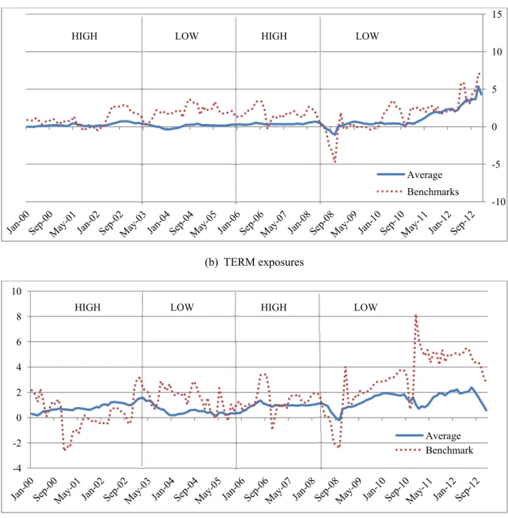
Figures 3a and 3b present the average DEF and TERM exposures of the equally-weighted funds as well as the benchmarks (passive portfolio). The sample period is from January 2000 to December 2012, and is partitioned into subperiods of high and low interest rates, where the cut-off point is the median one-month Euribor rate in the period (2.39%). The first high period (rates above the median rate) is from January 2000 until from April 2003, followed by a period of lower rates from May 2003 until January 2006 when rates begin to increase again and continue to do so from February 2006 until December 2008 and finally, in the aftermath of the financial crisis, a period of low rates from January 2009 until the end of the sample period. Default risk exposure is, on average, relatively flat and tends to be lower than the benchmark’s exposure. However, following the crisis the average default exposure jumps, as does that of the benchmark. Interest risk rate is more volatile, but the current pattern exists, until the financial crisis, when rates are low (high) the average fund’s risk exposure is lower (higher) than the benchmark’s. As was the case with default risk, interest rate risk also jumps following the crisis. This suggests that in the face of historically low rates funds seek historically high risk exposures in an attempt to generate returns.
Table 2 shows the cross-sectional distribution of the coefficients and t-statistics for the estimated alphas and betas of individual funds for equation (1), assuming the model parameters are static over time. Consistent with Gungor and Sierra (2014), on average, TERM is positive and statistically significant at the 5% level. However, DEF is positive but not statistically significant at the 5% level, only becoming statistically relevant at 10%. These results show that mutual funds in our sample take interest rate and default risk into account when generating excess returns.
while the factors used are not, this means that risk-adjusted returns are generally negative instead of being equal to zero (Fama and French (2010)). Table 2 shows that alpha is, on average, equal to -0.04 with a t-statistic equal to -3.25. The two-factor model explains, on average, 84%, of the changes in a typical fund’s excess return. This result is consistent with Gungor and Sierra (2014) who find that the two-factor model is responsible for 82% of the variation in their sample. Table 2 supports that the two-factor model is an acceptable characterization of the average risk-return relationship for my sample of fixed-income funds.
4.2 Risk Exposures and Monetary Policy
I then consider how the active risk exposure of an equally-weighted portfolio of funds reacts to the monetary policy proxies. The equally-weighted portfolio can be viewed as a representative fund and can describe the average changes in risk exposures. Table 3 shows the coefficient and
t-statistics estimates for the two-factor model: , , , , , .
The average fund has higher exposure to the TERM factor than to the DEF factor. When comparing the pre-crisis to the post-crisis data, it is clear that both term and default risk exposures have increased globally, which indicates that the mutual funds have not increased one exposure at the expense of another, but rather increased risk taking
Next, I study whether and how the active portion of risk exposure of an equally-weighted portfolio of funds reacts over time to monetary policy changes. I take the risk exposures of the equally-weighted portfolio and the benchmark previously estimated using a 24-month rolling window. Then for each of the risk factors (DEF and TERM), I run a regression in which the dependent variable is the risk factor of the equally-weighted portfolio, and the explanatory variables are the benchmark risk factor and the monetary policy variables (and control variables). The resulting estimated coefficients, t-statistics and R-squared for each risk factor, DEF and TERM, are presented in Tables 4 and 5, respectively. The tables present not only the full estimation period from January 2000 until December 2012 in Panel A but also two subperiods in Panels B and C for the period prior to the crisis (from January 2000 until December 2006) and the period following the crisis (from January 2007 to December 2012).
entire time period. The interpretation for this result is that the average fund exposes itself to greater default risk, meaning increasing the weight on high-yield debt in its portfolio, when interest rates fall and an expansionary monetary policy is in place. Additionally, Panel B and C consider whether this adjustment has changed due to the crisis and show that in fact this response to monetary policy is driven by the post-crisis period. Panel C shows that all of the monetary policy variables coefficients are negative and statistically significant, while in Panel B the coefficients are positive and statistically significant, with the exception of the first principal component. Thus, I conclude that it is exactly in the period with historically low interest rates that funds actively sought to increase the amount of default risk they were exposed to.
Table 5 shows the results for a similar analysis using interest rate risk as proxied by TERM. Over the entire sample period, the results vary. When considering the one-month Euribor rate and the policy rule residual, it seems that as interest rates go down funds seek to expose themselves to a greater degree of interest rate risk. However, when I consider the ex-post real rate, as interest rates go down then exposure decreases as well. The results become clearer when I compare the pre- and post-crisis period. When looking at the pre-crisis period, funds tend to decrease their interest rate risk as interest rates decrease, a result that is clear from the positive and statistically significant coefficients for the one-month Euribor rate, the policy rule residual, and the ex-post rule. This trend shifts after the crisis and during the period of historically low rates, as the average fund increases its interest rate risk in response to decreasing interest rates, as the aforementioned coefficients are negative and statistically significant.
In summary, the results indicate that when interest rates fall, the typical fund will expose itself to greater default and interest rate risk. This strategy to generate return via risk is adopted by Portuguese fixed-income mutual funds following the financial crisis and the monetary policy decisions made since then.
4.3 Individual Funds
cross-sectional information. For example, funds with differing coefficients and intercepts may cancel out within a portfolio subsequently leading to misleading conclusions and inference. Thus, individual funds are tested for active changes using the same two step procedure to assess whether the conclusions reached for the equally-weighted portfolio are robust.
Table 6 reports the cross-sectional distribution of the estimated coefficients and respective
t-statistics resulting from the breakdown of , . On average, consistent with the equally-weighted portfolio, the coefficients are all negative and statistically significant at the 5% level with the exception of the first principal component. Also, the heteroskedasticity and serial-correlation robust generalized method of moments (GMM) is used to test for joint significance and strongly rejects the null hypothesis that funds do not to actively adjust their risk exposures to changes in monetary policy. The average DEF exposure of funds from Table 6 is equal to 0.55 suggesting that a decrease of 10 basis points in the one-month interest rate would render a 12.57% higher default risk exposure. Across the 54 individual funds in my sample, at least 10 have a statistically significant negative coefficient, peaking at 13 when the proxy is the ex-post real rate. This indicates that approximately 24% of the funds adjust their exposure to default risk negatively and statistically significantly to increasing policy rates. However, it should also be noted that across the alternative proxies at least six funds had positive reactions meaning that active exposure increases in response to increases in policy rates, peaking at 19, which is approximately 27.7%, when the policy rule residual is considered. Overall, the interpretation is that on average individual funds react to declines in interest rates and expansionary monetary policies by boosting active default risk exposure.
default risk exposures. The peaks of statistically significant non-zero coefficients are 21 out of 54 funds (38.9%) with positive non-zero one-month rate coefficients and 19 out of 54 (27.8%) funds with negative non-zero coefficients for the policy rule residual. When considering the average number of funds that are statistically significant across all four alternative monetary variables, the average is higher for negative and statistically significant, indicating that the reaction of boosting interest rate risk exposure in response to falling rates is slightly stronger than decreasing risk as a response.
Individual fund data seems to support the original equally-weighted portfolio findings suggesting that Portuguese fixed-income mutual funds clearly increase default risk exposure in response to a decrease in interest rates and expansionary monetary policies. Funds are also found to slightly increase their interest rate risk exposures in response to rate cuts.
4.4 Economic Significance
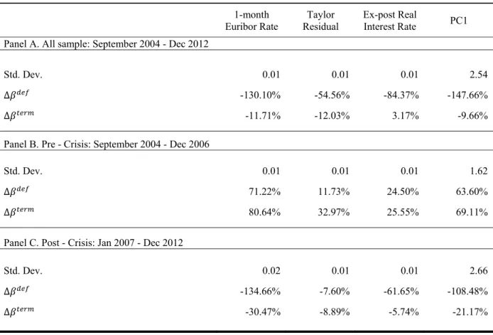
In addition to considering the statistical relevance of the findings, in order to complement my findings I will also consider the economic significance of the results. Table 8 presents the percentage change in risk exposure (DEF and TERM) given a one-standard deviation change in monetary policy variables. Panel A presents the estimates over the entire sample period. It is clear that default and interest rate risk exposures move in the same direction, albeit the change in default risk exposure is greater than that of interest risk rate. This is clear when one considers the average across all monetary policy alternatives, which is approximately 104% for default risk compared to interest rate risk’s 7.5%.
Conclusion
This paper shows that Portuguese fixed-income mutual funds increase their exposure to default risk and to some extent, however less apparent, their exposure to interest risk rate, in response to expansionary monetary policies and interest rate cuts.
Using a linear two-factor pricing model, I estimate the dynamic risk exposures for individual funds, the benchmarks as well as for a representative equally-weighted portfolio. I then link these time-varying risk exposures to the benchmark’s exposure, which is indicative of the passive exposure, as well as macroeconomic variables. The results show that the individual fund’s exposure to both default and interest rate risk is not significantly explained by the benchmark’s exposure which indicates that the majority of funds, on average, seek to expose themselves to default risk, and somewhat to interest rate risk, as an active response to monetary policy. When I consider a representative equally-weighted portfolio I obtain similar results of statistically significant active portion of risk exposures increasing in reaction to accommodative monetary policy stances. Interestingly, the results clearly show a change in strategy following the 2007-2009 financial crisis. While prior to the crisis, Portuguese fixed-income mutual funds actually decrease their risk exposures when interest rates fall, in the aftermath of the crisis they then shifted this response to increase risk when rate cuts occur suggesting that the current historically low rates induce extra-risk taking unseen before.
References
Abramowicz, L. (2014). Banco Espirito Santo Loan Mystery Confronts Derivatives Buyers.
Bloomberg.
Alloway, T. (2014). US banks warn on ‘excessive’ risk-taking. The Financial Times.
Ang, A. and D. Kristensen (2012). Testing conditional factor models. Journal of Financial
Economics 106 (1), 132-156.
Ang, A., J. Liu, and K. Schwarz (2010). Using stocks or portfolios in tests of factor models. Working Paper, Columbia University.
Authers, J. (2014). Risk-return relationship has been upended. The Financial Times. Bank of England (2013). Financial Stability Report.
Becker, B., and V. Ivashina. (2014). Reaching for Yield in the Bond Market. forthcoming,
Journal of Finance .
Bekaert, G., M. Hoerova, and M. L. Duca (2013). Risk, uncertainty and monetary policy.
Journal of Monetary Economics 60 (7), 771-788.
Chen, Y. and N. Qin (2014). The Behavior of Investor Flows in Corporate Bond Mutual Funds. Working Paper.
Chevalier, J. and G. Ellison (1999). Career concerns of mutual fund managers. The Quarterly Journal of Economics 114 (2), 389-432.
Choi, J. and Kronlund, M (2014). Reaching for Yield or Playing It Safe? Risk Taking by Bond Mutual Funds. Working Paper, University of Illinois.
Cici, G., and S. Gibson (2012) The Performance of Corporate Bond Mutual Funds: Evidence Based on Security-Level Holdings. Journal of Financial and Quantitative Analysis 47,159-178. Cici, G., S. Gibson, and J. Merrick (2011). Missing the marks? Dispersion in corporate bond valuations across mutual funds. Journal of Financial Economics 101, 206-226.
Cremers, K. J. M. and A. Petajisto (2009). How active is your fund manager? A new measure that predicts performance. Review of Financial Studies 22 (9), 3329-3365.
Deutsche Bundesbank (2014). Financial Stability Review.
Estrella, A. and G. Hardouvelis (1991). The term structure as a predictor of real economic activity. The Journal of Finance 46, 555-576.
European Fund and Asset Management Association (2013). EFAMA International Statistical Release (2012:Q4).
European Securities and Markets Authority (2014). Trends, Risks, Vulnerabilities No. 1, 2014. European Securities and Markets Authority (2014). Trends, Risks, Vulnerabilities No. 2, 2014. Fama, E. and R. Bliss (1987). The information in long-maturity forward rates. American
Economic Review 77, 680-692.
Fama, E. and K. French (1993). Common risk factors in the returns on stocks and bonds. Journal
of Financial Economics 33, 3-56.
Fama, E. and K. French (2010). Luck versus skill in the cross-section of mutual fund returns. The
Journal of Finance 65 (5), 1915-1947.
Ferson, W. and R. Schadt (1996). Measuring fund strategy and performance in changing economic conditions. The Journal of Finance 51, 425-461.
Gambacorta, L. (2009). Monetary policy and the risk-taking channel. BIS Quarterly Review
(December), 43-53.
Gungor, S. and Sierra, J. (2014). Search-for-Yield in Canadian Fixed-Income Mutual Funds and Monetary Policy. Bank of Canada Working Paper 2014-3.
Ioannidou, V., S. Ongena, and J. Peydró (2010). Monetary policy, risk-taking and pricing: Evidence from a quasi-natural experiment. CentER Discussion Paper Series No. 2009-31S. IOSCO (2014). Securities Market Risk Outlook 2014-15.
Jimenez, G., S. Ongena, J. Peydró, and J. Saurina (2008). Hazardous times for monetary policy: What do twenty-three million bank loans say about the effects of monetary policy on credit risk-taking? Banco de España Working Paper No. 833.
Joint Committee for European Supervisory Authority (2014). Report on Risk and Vulnerabilities in the EU Financial System.
Jones, C. (2014). Bundesbank warns corporate debt becoming overpriced. The Financial Times.
Rajan, R. (2010). Fault Lines. Princeton University Press.
Roll, R. (1977). A critique of the asset pricing theory tests; part i: On past and potential testability of the theory. Journal of Financial Economics 4, 129-176.
Turner, M. (2014). European high-yield bond market hits its stride. Financial News.
Pictet Asset Management (2014). What now for European high-yield bonds?
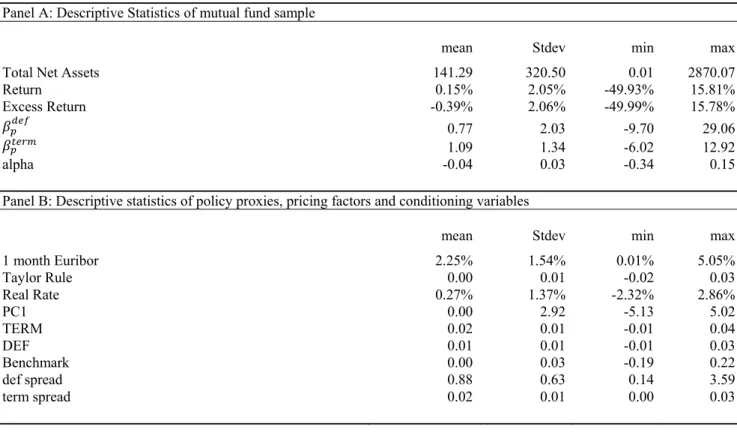
Table 1: Descriptive statistics
Panel A: Descriptive Statistics of mutual fund sample
mean Stdev min max
Total Net Assets 141.29 320.50 0.01 2870.07
Return 0.15% 2.05% -49.93% 15.81%
Excess Return -0.39% 2.06% -49.99% 15.78%
0.77 2.03 -9.70 29.06
1.09 1.34 -6.02 12.92
alpha -0.04 0.03 -0.34 0.15
Panel B: Descriptive statistics of policy proxies, pricing factors and conditioning variables
mean Stdev min max
1 month Euribor 2.25% 1.54% 0.01% 5.05%
Taylor Rule 0.00 0.01 -0.02 0.03
Real Rate 0.27% 1.37% -2.32% 2.86%
PC1 0.00 2.92 -5.13 5.02
TERM 0.02 0.01 -0.01 0.04
DEF 0.01 0.01 -0.01 0.03
Benchmark 0.00 0.03 -0.19 0.22
def spread 0.88 0.63 0.14 3.59
term spread 0.02 0.01 0.00 0.03
Table 2: CrossSectional distribution of two-factor model coefficient estimates: Individual funds
Coefficient Estimates t-statistics R2
alpha TERM DEF alpha TERM DEF
Minimum -0.34 -6.02 -9.70 -1861.52 -759.02 -2437.36 0.00
Average -0.04 1.09 0.77 -3.25 2.11 1.29 0.84
Maximum 0.15 12.92 29.06 0.94 2.13 2.63 0.99
No. of funds 90
No. of funds with <0 alpha 79
No. of funds with >0 alpha 11
No. of funds with <0 alpha significant at 5% 19 No. of funds with >0 alpha significant at 5% 10
This table shows the cross-sectional distribution of the coefficients and their t-statistics for the individual funds
within the sample estimated using the unconditional two-factor model: , , , ,
,, where both the intercept and factors are held constant overtime. The remaining rows summarize the funds that
have intercepts that are statistically significant and different from zero.
Table 3: Two-factor coefficient estimates: single equally-weighted portfolio
alpha TERM DEF N R2
All Sample: Jan 2000 - Dec 2012 -0.05 1.46 0.61 156 0.40
-17.97 10.32 3.98
Pre-Crisis: Jan 2000 - Dec 2006 -0.04 1.14 0.39 84 0.72
-19.50 9.05 2.75
Post-Crisis: Jan 2007 - Dec 2012 -0.05 1.49 0.58 72 0.95
-8.51 9.02 1.71
This table shows the values of the coefficients and their t-statistics for the unconditional two-factor model: ,
, , , , tested on an equally-weighted portfolio of all funds in the sample and
Table 4: Explaining : single equally-weighted portfolio 1-month Euribor Rate Taylor Residual Ex-post Real
Interest Rate PC1
Panel A. All sample: September 2004 - Dec 2012
monetary policy -69.43 -44.19 -49.21 -0.45
(26.82) (42.32) (15.62) (0.09)
benchmark 0.34 0.42 0.32 0.26
(0.09) (0.12) (0.08) (0.07)
term spread -79.23 -0.18 -27.94 -75.53
(40.79) (17.83) (19.06) (22.19)
default spread 0.53 0.45 0.59 0.33
(0.23) (0.28) (0.21) (0.16)
constant 2.36 -0.66 0.17 1.03
(1.09) (0.37) (0.28) (0.37)
N 99 99 99 99
R2 10.71% 14.01% 8.60% 18.94%
Panel B. Pre - Crisis: September 2004 - Dec 2006
monetary policy 17.33 2.46 5.73 0.09
(6.57) (5.55) (2.99) (0.02)
benchmark 0.05 0.36 0.05 0.04
(0.01) (0.03) (0.02) (0.01)
term spread 6.01 -10.46 -2.98 2.67
(7.67) (5.02) (6.70) (4.29)
default spread -0.17 -0.18 -0.20 -0.11
(0.03) (0.04) (0.04) (0.02)
constant -0.22 0.06 0.28 0.18
(0.24) (0.02) (0.05) (0.05)
N 27 27 27 27
R2 81.60% 53.31% 76.83% 77.90%
Panel C. Post - Crisis: Jan 2007 - Dec 2012
monetary policy -99.38 -17.05 -49.96 -0.48
(17.78) (41.95) (12.70) (0.07)
benchmark 0.34 0.50 0.37 0.28
(0.06) (0.10) (0.07) (0.06)
term spread -135.83 1.29 -35.70 -92.03
(33.70) (18.32) (20.58) (18.62)
default spread 0.49 0.32 0.53 0.24
(0.17) (0.26) (0.19) (0.15)
constant 4.23 -0.32 0.48 1.55
(0.87) (0.37) (0.28) (0.32)
N 72 72 72 72
R2 38.28% 20.43% 29.99% 45.99%
This tables shows the results obtained from , , , , , ,,
Table 5: Explaining : single equally-weighted portfolio 1-month Euribor Rate Taylor Residual Ex-post Real
Interest Rate PC1
Panel A. All sample: September 2004- Dec 2012
monetary policy -8.81 -13.73 2.60 -0.04
(14.56) (20.49) (7.85) (0.08)
benchmark 0.18 0.17 0.19 0.17
(0.07) (0.07) (0.07) (0.08)
term spread -2.11 5.20 11.85 2.31
(22.42) (12.19) (13.14) (18.30)
default spread 0.09 0.09 0.04 0.06
(0.13) (0.13) (0.14) (0.12)
constant 0.84 0.46 0.46 0.62
(0.65) (0.14) (0.18) (0.31)
N 99 99 99 99
R2 14.47% 11.09% 11.99% 15.15%
Panel B. Pre - Crisis: September 2004 - Dec 2006
monetary policy 62.83 22.14 19.14 0.30
(7.75) (24.84) (12.15) (0.05)
benchmark 0.11 0.16 0.14 0.11
(0.02) (0.04) (0.03) (0.02)
term spread 17.30 -34.77 -15.11 -0.45
(10.76) (7.58) (15.34) (12.00)
default spread -0.36 -0.42 -0.47 -0.15
(0.22) (0.20) (0.23) (0.13)
constant -1.04 1.13 0.79 0.44
(0.24) (0.08) (0.24) (0.08)
N 27 27 27 27
R2 73.03% 80.71% 82.98% 85.21%
Panel C. Post - Crisis: Jan 2007 - Dec 2012
monetary policy -26.24 -23.27 -5.43 -0.11
(17.26) (15.49) (7.82) (0.09)
benchmark 0.09 0.11 0.11 0.07
(0.08) (0.08) (0.08) (0.09)
term spread -19.59 8.16 12.90 -2.63
(23.69) (9.75) (11.24) (17.78)
default spread 0.02 0.02 -0.02 -0.05
(0.11) (0.13) (0.13) (0.10)
constant 1.90 0.69 0.82 1.14
(0.79) (0.13) (0.19) (0.37)
N 72 72 72 72
R2 1.55% 17.57% 17.51% 19.88%
This tables shows the results obtained from , , , , ,
, , where , measures portfolio p’s exposure to interest rate risk at time t, , is benchmark’s exposure to
Table 6: The cross-sectional distribution of t-statistics for the monetary policy indicators: Default-risk exposure in individual funds
1-month rate Taylor real rate pc1
Coeff t-stat Coeff t-stat Coeff t-stat Coeff t-stat
Minimum -283.81 0.86 -285.41 1.36 -386.69 0.85 -2.18 1.17
Average 29.73 27.78 15.27 27.96 -6.26 15.67 0.09 0.11
Maximum 382.11 381.29 596.41 365.77 170.63 155.65 1.01 0.01
GMM -35.47 -46.65 -32.52 -0.20
p-value 0.0000 0.0330 0.0000 0.0000
No and % of funds
t-stat < -2.58 18 8 16 14
33.33% 14.81% 29.63% 25.93%
-2.58 < t-stat < -1.96 1 5 3 6
1.85% 9.26% 5.56% 11.11%
-1.96 < t-stat < -1.65 3 5 3 3
5.56% 9.26% 5.56% 5.56%
-1.65 < t-stat < 0 12 10 13 12
22.22% 18.52% 24.07% 22.22%
0 < t-stat < 1.65 7 19 6 6
12.96% 35.19% 11.11% 11.11%
1.65 < t-stat < 1.96 2 1 3 1
3.70% 1.85% 5.56% 1.85%
1.96 < t-stat < 2.58 2 1 3 1
3.70% 1.85% 5.56% 1.85%
2.58 < t-stat 9 5 7 11
16.67% 9.26% 12.96% 20.37%
Total no. of funds 54 54 54 54
No. of significantly <0 fund 12 10 13 12
No. of significantly >0 fund 7 19 6 6
This table shows the cross-sectional distribution of the estimated coefficient and respective t-statistics at a fund-level
for the following regression: , , , , , , , which breaks a
Table 7: The cross-sectional distribution of t-statistics for the monetary policy indicators: Default-risk exposure in individual funds
1-month rate Taylor real rate pc1
Coeff t-stat Coeff t-stat Coeff t-stat Coeff t-stat
Minimum -461.19 0.71 -366.80 1.45 -202.97 0.67 -2.19 0.01
Average 23.34 26.49 4.82 27.65 4.30 16.09 0.06 0.12
Maximum 636.33 192.70 727.75 181.22 177.21 132.28 1.43 1.04
GMM 5.27 0.86 15.53 0.05
p-value 0.1630 0.9010 15.5254 0.0060
No and % of funds
t-stat < -2.58 5 3 4 8
9.26% 5.56% 7.41% 14.81%
-2.58 < t-stat < -1.96 3 3 1 2
5.56% 5.56% 1.85% 3.70%
-1.96 < t-stat < -1.65 3 3 1 2
5.56% 5.56% 1.85% 3.70%
-1.65 < t-stat < 0 7 19 8 8
12.96% 35.19% 14.81% 14.81%
0 < t-stat < 1.65 21 15 11 13
38.89% 27.78% 20.37% 24.07%
1.65 < t-stat < 1.96 0 2 4 1
0.00% 3.70% 7.41% 1.85%
1.96 < t-stat < 2.58 6 4 4 6
11.11% 7.41% 7.41% 11.11%
2.58 < t-stat 9 5 21 14
16.67% 9.26% 38.89% 25.93%
Total no. of funds 54 54 54 54
No. of significantly <0 fund 7 19 8 8
No. of significantly >0 fund 21 15 11 13
This table shows the cross-sectional distribution of the estimated coefficient and respective t-statistics at a fund-level
for the following regression: , , , , , ,, which
Table 8: Economic significance: single equally-weighted portfolio
1-month Euribor Rate
Taylor Residual
Ex-post Real
Interest Rate PC1
Panel A. All sample: September 2004 - Dec 2012
Std. Dev. 0.01 0.01 0.01 2.54
∆ -130.10% -54.56% -84.37% -147.66%
∆ -11.71% -12.03% 3.17% -9.66%
Panel B. Pre - Crisis: September 2004 - Dec 2006
Std. Dev. 0.01 0.01 0.01 1.62
∆ 71.22% 11.73% 24.50% 63.60%
∆ 80.64% 32.97% 25.55% 69.11%
Panel C. Post - Crisis: Jan 2007 - Dec 2012
Std. Dev. 0.02 0.01 0.01 2.66
∆ -134.66% -7.60% -61.65% -108.48%
∆ -30.47% -8.89% -5.74% -21.17%
Figure 1: Monetary Policy Proxies
This figure presents the four alternative monetary policy proxies used in the analysis: the one-month Euribor rate, the ex-post real rate, the policy rule residual (also known as the Taylor rule) and the first principal component of a cross-section of yields of different maturity German bunds and Euribor rates.
Figure 2: Average Fund Return Volatility
This figure depicts average volatility of the fund returns, in local currency, within the sample. The volatility was computed using a 24-month rolling window on the monthly return data.
-6 -4 -2 0 2 4 6 -0,03 -0,02 -0,01 0 0,01 0,02 0,03 0,04 0,05 0,06 Real rate Taylor Rule 1-month rate PC1 0,00% 0,50% 1,00% 1,50% 2,00% 2,50% 3,00% 3,50% Feb -99 Au g-99 Feb -00 Au g-00 Feb -01 Au g-01 Feb -02 Au g-02 Feb -03 Au g-03 Feb -04 Au g-04 Feb -05 Au g-05 Feb -06 Au g-06 Feb -07 Au g-07 Feb -08 Au g-08 Feb -09 Au g-09 Feb -10 Au g-10 Feb -11 Au g -1 1 Feb -12 Au g-12 Lehman Brothers Beginning
Figure 3: Time-varying risk exposures
(a) DEF exposures
(b) TERM exposures
This figure presents the rolling betas for both DEF and TERM estimated with a 24-month rolling window across the time frame from January 2000 to December 2012. The solid line refers to the average risk exposure of all the funds in the sample and the dotted line shows the risk exposure of the benchmark. The time frame is partitioned into subperiods of high and low interest rates, where the cut-off point is the median interest in the period (2.39%). The first high period (rates above the median rate) is from Jan. 2000 until from Apr. 2003, followed by a period of lower rates from May 2003 until Jan. 2006 when rates begin to increase again and continue to do so from Feb. 2006 until Dec. 2008 and finally, in the aftermath of the financial crisis a period of low rates from Jan. 2009 until the end of the time frame.
-10 -5 0 5 10 15
Average
Benchmarks
HIGH LOW HIGH LOW
-4 -2 0 2 4 6 8 10
Average Benchmark