Finite probability distributions in Coq

(1)

(2)

(3)

(4)

(5)

not enough; we must do. Johann Wolfgang von Goethe

(6)

Acknowledgements

To my supervisor, Professor José Carlos Bacelar Almeida, for the support, exper-tise and careful guidance provided throughout this work, a special thanks for everything.

To all the people involved in the SMART project at Minho’s University, in par-ticular: Manuel Barbosa, José Barros, Manuel Alcino, Paulo Silva, Luís Miranda and Tiago Oliveira, for all the fruitful discussions and good working environment provided, a sincere thank you. During the execution of this work, I was given a research grant - Bolsa de Investigação Científica (BIC), funded by the ENIAC JU program (GA 120224).

To my home town friends, for understanding the countless times I did not show up for our weekly meetings, for the continuous support and friendship, thank you for never letting me down.

To my friends in Braga, but specially to my friends at Confraria do Matador, a huge thanks for this 5 years of great experiences.

To Sara and Sérgio, I am extremely grateful for all the help provided in the elaboration of this document.

To all my family, but specially to my parents, José and Maria, and my brother, Ricardo, words cannot describe how much you mean to me. A huge thank you from the bottom of my heart, for being my guiding light and source of inspiration, and for providing the conditions that allowed me to be where I am at this stage of my life.

(7)

(8)

Abstract

When building safety-critical systems, guaranteeing properties like correctness and security are one of the most important goals to achieve. Thus, from a sci-entific point of view, one of the hardest problems in cryptography is to build systems whose security properties can be formally demonstrated.

In the last few years we have assisted an exponential growth in the use of tools to formalize security proofs of primitives and cryptographic protocols, clearly showing the strong connection between cryptography and formal methods. This necessity comes from the great complexity and sometimes careless presentation of many security proofs, which often contain holes or rely on hidden assump-tions that may reveal unknown weaknesses. In this context, interactive theorem provers appear as the perfect tool to aid in the formal certification of programs due to their capability of producing proofs without glitches and providing addi-tional evidence that the proof process is correct.

Hence, it is the purpose of this thesis to document the development of a frame-work for reasoning over information theoretic concepts, which are particularly useful to derive results on the security properties of cryptographic systems. For this it is first necessary to understand, and formalize, the underlying probability theoretic notions. The framework is implemented on top of the fintype and finfun modules of SSREFLECT, which is a small scale reflection extension for the COQ proof assistant, in order to take advantage of the formalization of big operators and finite sets that are available.

(9)

(10)

Resumo

Na construção de sistemas críticos, a garantia de propriedades como a correção e segurança assume-se como um dos principais objetivos. Deste modo, e de um ponto de vista científico, um dos problemas criptográficos mais complicados é o de construir sistemas cujas propriedades possam ser demonstradas formalmente. Nos últimos anos temos assistido a um crescimento enorme no uso de fer-ramentas para formalizar provas de segurança de primitivas e protocolos crip-tográficos, o que revela a forte ligação entre a criptografia e os métodos formais. Urge esta necessidade devido à grande complexidade, e apresentação por vezes descuidada, de algumas provas de segurança que muitas vezes contêm erros ou se baseiam em pressupostos escondidos que podem revelar falhas desconheci-das. Desta forma, os provers interativos revelam-se como a ferramenta ideal para certificar programas formalmente devido à sua capacidade de produzir provas sem erros e de conferir uma maior confiança na correção dos processos de prova. Neste contexto, o propósito deste documento é o de documentar e apresentar o desenvolvimento de uma plataforma para raciocinar sobre conceitos da teoria de informação, que são particularmente úteis para derivar resultados sobre as propriedades de sistemas criptográficos. Para tal é necessário, em primeiro lugar, entender e formalizar os conceitos de teoria de probabilidades subjacentes. A plataforma é implementada sobre as bibliotecas fintype e finfun do SSREFLECT, que é uma extensão à ferramenta de provas assistas COQ, por forma a aproveitar a formalização dos somat’ orios e conjuntos finitos disponíveis.

(11)

(12)

List of Figures

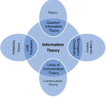
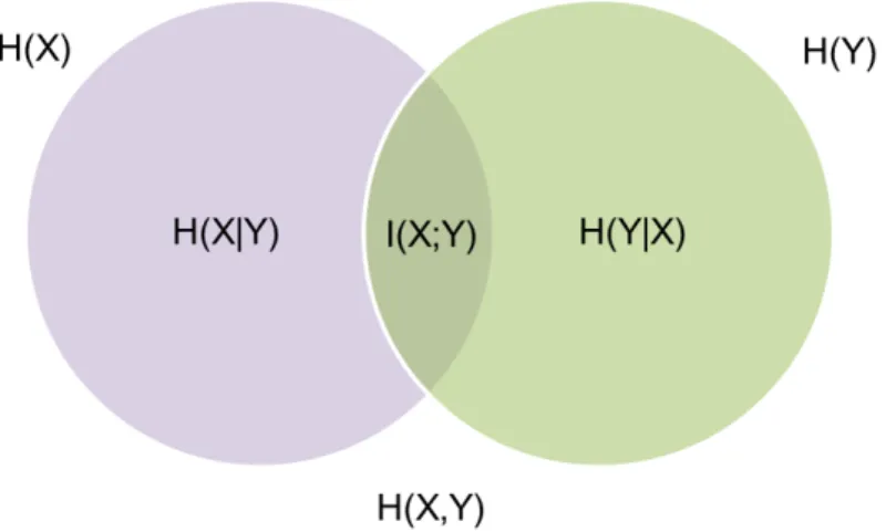
3.1 Venn diagram for set operations: union, intersection and comple-ment. . . 23 5.1 Relationship of information theory to other fields. . . 48 5.2 Graphical representation of the relation between entropy and

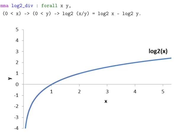
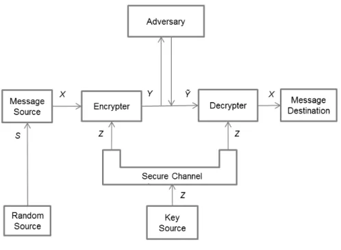
mu-tual information. . . 53 6.1 Graph of the logarithm to the base 2. . . 63 6.2 Generalization of Shannon’s model of a symmetric cipher. . . 71

(17)

(18)

Chapter 1 Introduction

Number theory and algebra have been playing an increasingly significant role in computing and communications, as evidenced by the striking applications of these subjects in fields such as cryptography and coding theory [Sho05]. How-ever, the commonly held opinion is that the formalization of mathematics is a long and difficult task for two reasons: first, standard mathematical proofs (usu-ally) do not offer a high enough level of detail and second, formalized theory is often insufficient as a knowledge repository which implies that many lemmas have to be reproved in order to achieve relevant results.

In the last few years we have assisted an exponential growth in the use of tools to formalize security proofs of primitives and cryptographic protocols, clearly showing the strong connection between cryptography and formal methods. This necessity comes from the great complexity and sometimes careless presentation of many important scheme’s proofs, which may lead to mistakes undetected un-til now. Moreover, and although provable cryptography provides high assurable cryptographic systems, security proofs often contain glitches or rely on hidden assumptions that may reveal unknown weaknesses. In this context, interactive theorem provers appear as the perfect tool to aid in the formal certification of pro-grams due to their capability to produce proofs without the holes usually found in their paper versions and to provide additional evidence that the proof process is correct. This idea is reflected by the increasing use, despite some may think, of interactive theorem provers for industrial verification projects: for instance,

(19)

NASA uses PVS1to verify software for airline control and Intel uses HOL light2 to verify the design of new chips [Geu09].

Cryptographic protocols provide mechanisms to ensure security that are used in several application domains, including distributed systems and web services (and more recently also in the protection of intellectual property). However, de-signing secure cryptographic protocols is extremely difficult to achieve [BT05]. In this context there is an increasing trend to study such systems, where the specifi-cation of security requirements is provided in order to establish that the proposed system meets its requirements.

Thus, from a scientific point of view, one of the most challenging problems in cryptography is to build systems whose security properties can be formally demonstrated. Such properties only make sense in a context where a definition of security is given: furthermore, knowledge about the adversary’s available infor-mation and computation power should also be provided. Both adversary and be-nign entity are probabilistic processes that communicate with each other, and so, it is possible to model this environment as a probability space. Equally important, we may use information (and probability) theoretic concepts (e.g., entropy) to de-rive results on the security properties of cryptographic systems, which clearly reflects the fundamental role of these two areas in cryptography [Mau93].

1.1 Objectives

The central objective of this work is to build a framework that provides the user the possibility to reason over information theory concepts, particularly in the field of cryptography. Thus, it is first necessary to understand, and formalize, the underlying probability theory notions and also how to use them in order to build such framework. In this context we aim to develop, in COQ, a library that formalizes fundamental laws of probability theory and basic concepts of infor-mation theory.

1_{http://pvs.csl.sri.com/}

(20)

1.2. CONTRIBUTIONS 3

1.2 Contributions

This thesis proposes a formal framework to reason about probability and infor-mation theory concepts, possibly in a cryptographic environment, which is im-plemented using the COQ proof assistant, and particularly, the SSREFLECT plu-gin. The key to our implementation is to take advantage of the formalization of big operators and finite sets provided by the SSREFLECTlibraries finset and bigop, since it allows to precisely capture the mathematical aspects of the concepts in-volved.

In detail, we make the following contributions:

• Development of a probability oriented framework

A COQframework is implemented that allows the user to reason about ba-sic notions of probability and set theory.

• Extension of the framework to include the formalization of relevant in-formation theoretic concepts

On top of the probability oriented frame work, a formalization of infor-mation theory concepts is added that should serve as a basis to reason in cryptographic contexts.

1.3 Dissertation Outline

The remainder of the document is organized as follows: Chapter 2 briefly intro-duces the COQ proof assistant, its small scale reflection extension, SSREFLECT and the two most relevant libraries for this work; Chapter 3 explains basic con-cepts of probability theory; Chapter 4 discusses our approach to the formalization of discrete probabilities in COQ; Chapter 5 introduces important notions of infor-mation theory with a focus on the concept of entropy; Chapter 6 presents and discusses our formalization of such information theoretic concepts. The Chapter closes with a simple case study.

(21)

(22)

Chapter 2 Interactive Theorem Proving

“For our intention is to provide a medium for doing mathematics different from that provided by paper and blackboard. Eventually such a medium may support a variety of input devices and may provide communication with other users and systems; the essential point, however, is that this new medium is active, whereas paper, for example, is not."

Constable et al. [CAA+_86] An interactive theorem prover, or proof assistant, is a software tool that aids in the development of formal proofs by interacting with the user (user-machine collaboration). Its purpose is to show that some statement, the conjecture, is a logical consequence of a set of statements, the axioms and hypotheses, given an appropriate formalization of the problem.

These statements are written using a logic (e.g., first-order logic, high-order logic), which enables the user to formulate the problem in such a way that the machine may, unambiguously, understand it. The idea is to allow him to set up a mathematical context, define properties and logically reason about them. The user then guides the search for proofs in a proof editing mode where he should be relieved of trivial steps in order to concentrate on the decision points of the proofs. Therefore the system must provide a large, and trusted, set of mathemat-ical theory which usually represents a measure of the success of the system and serves as a means of achieving complex results. In practice, for serious formaliza-tion of mathematics a good library is usually more important than a user friendly

(23)

system.

The input language of a proof assistant can be declarative, where the user tells the system where to go, or procedural, where the user tells the system what to do [Geu09]. Usually the proofs of the latter are not readable by the common reader since they only have meaning for the proof assistant whereas the proofs of the former tend to be written in a more clear and natural way. This is exemplified by the fact that proof scripts1_{need not correspond to a proof in logic, as generally} happens with procedural proofs but not with declarative proofs.

In mathematics, and in particular when dealing with proof assistants, a proof is absolute. It is the mathematical validation of a statement, whose correction can be determined by anyone, and is supposed to both convince the reader that the statement is correct and to explain why it is valid. Each proof can be divided in small steps that may be individually verified. This is important when handling the proof of a theorem that turns out to be false as it allows to pinpoint the exact step(s) that cannot be verified.

Nowadays proof assistants are mainly used by specialists who seek to formal-ize theories in it and prove theorems. In fact the community of people formalizing mathematics is relatively small and is spread across the existent proof assistants. This chapter starts by giving a brief overview about the interactive theorem prover COQ, namely: its specification language, proof process, canonical struc-tures mechanism and standard library. The chapter closes by introducing a small scale reflection extension to the COQproof system called SSREFLECTand its most important libraries for the purposes of this work, finset and bigop.

2.1 The C

OQ

Proof Assistant

The COQsystem [Teaa] is an interactive theorem prover whose underlying formal language is based on an axiom-free type theory called the Calculus of Inductive Constructions2. Its core logic is intuitionistic but it can be extended to a classical logic by importing the correct module. Laws like the excluded middle, A∨ ¬A, or the double negation elimination,¬¬A⇒ A, will then become available.

1_{proofs done using a proof assistant}

(24)

2.1. THE COQ PROOF ASSISTANT 7 As a programming language it is capable to express most of the programs al-lowed in standard functional languages (one of the exceptions being the inability to express non-terminating programs which enforces restrictions on the recursion patterns allowed in the definitions).

As a proof assistant, it is designed to allow the definition of mathematical and programming objects, writing formal proofs, programs and specifications that prove their correctness. Thus, it is a well suited tool for developing safe programs but also for developing proofs in a very expressive logic (i.e., high order logic), which are built in an interactive manner with the aid of automatic search tools when possible. It may also be used as logical framework in order to implement reasoning systems for modal logics, temporal logics, resource-oriented logics, or reasoning systems on imperative programs [BC04].

2.1.1 The Language

COQobjects represent types, propositions and proofs which are defined in a spec-ification language, called Gallina, that allows the user to define formulas, verify that they are well-formed and prove them. However, it comprises a fairly ex-tensive syntax and so we only touch a few important aspects (see [The06] for a complete specification of the Gallina language).

Every object is associated to (at least) a type and each type is an object of the system. This means that every well-formed type has a type, which in turn has a type, and so on3. The type of a type is always a constant and is called a sort. For instance

true : bool 0 : nat

S : nat -> nat

where nat is the type for natural numbers and bool contains two constants asso-ciated with truth values (true and false). Hence all objects are sorted into two categories:

• Prop is the sort for logical propositions (which, if well-formed, have type

3_{this happens because all types are seen as terms of the language and thus should belong to}

(25)

Prop). The logical propositions themselves are the types of their proofs; • Set intends to be the type for specifications (i.e., programs and the usual

datatypes seen in programming languages such as booleans, naturals, etc).

Since sorts should be given a type, a Type(0) is added as the type of sorts Set and Prop (among others). This sort, in turn, has type Type(1), and so on. This gives rise to a comulative hierarchy of type-sorts Type(i), for all i ∈ N. Such a hierarchy avoids the logical inconsistencies that result from considering an axiom such asType:Type[The06]. Note however that, from the user perspective, the indices of the Type(i) hierarchy are hidden by the system, and treated as constraints that are inferred/imposed internally.

Useful COQtypes are:

nat type of natural numbers (e.g., 6:nat) bool type of boolean values (e.g., true:bool)

Prop type of propositions

Type(orSet) type of types (e.g., nat:Set) T1 -> T2 type of functions from T1 to T2

T1 * T2 type of pairs of type T1 and T2

COQ syntax for logical propositions is summarized by (first row presents the mathematical notation and the second row presents the corresponding COQ no-tation):

⊥ � x=y x_�= y _¬P P_∨Q P_∧Q P _⇒Q P_⇔ Q False True x = y x <> y ~ P P \/ Q P /\ Q P -> Q P <-> Q Note that the arrow (->) associates to the right and so propositions such as T1 -> T2 -> T3 are interpreted as T1 -> (T2 -> T3).

Finally we show the syntax for universal and existential quantifiers:

∀x, P ∃x, P

forall x, P exists x, P

(26)

2.1. THE COQ PROOF ASSISTANT 9 The type annotation :T may be omitted if T can be inferred by the system. Universal quantification serves different purposes in the world of COQ as it can be used for first-order quantification like in forall x:T, x = x or for higher-order quantification like inforall (A:Type)(x:A), x = x orforall A:Prop, A -> A. Actually, both the functional arrow and the logical implication are special cases of universal quantifications with no dependencies (e.g., T1 -> T2 states the same asforall _:T1, T2).

2.1.2 Proof Process

Like in almost every programming language’s compiler, the core of the COQ sys-tem is a type checker, i.e., an algorithm which checks whether a formula is well-formed or not. Actually it is the way COQ checks proofs’ correctness: proving a lemma may be seen as the same as proving that a specific type is inhabited. This is explained by the fact that COQ sees logical propositions as the type of their proofs, meaning that if we exhibit an inhabitant of T:Prop, we have given a proof of T that witnesses its validity [Ber06]. This is the essence of the well known Curry-Howard isomorphism.

Proof development is carried in the proof editing mode through a set of com-mands called tactics4_{that allow a collaborative (user-machine) proof process. The} proof editing mode is activated when the user enunciates the theorem, using the TheoremorLemmacommands. These commands generate a top-level goal that the user will then try to demonstrate. In each step of the process there is a list of goals to prove that are generated by the tactics applied in the step before. When there are no goals remaining (i.e., the proof is completed) the command Qedwill build a proof term from the tactics that will be saved as the definition of the theorem for further reuse.

COQ’s proof development process is intended to be user guided but it still provides some kind of automatisation through a set of advanced tactics to solve complex goals. For instance:

• auto: Prolog style inference, solves trivial goals. Uses the hints from a

4_{a tactic is a program which transforms the proposition to be proved (goal) in a set of (possibly}

(27)

database, which can be extended by the user;

• tauto: complete for (intuitionistic) propositional logic;

• ring: solves equations in a ring or semi-ring structure by normalizing both hand sides of the equation and comparing the results;

• fourier: solves linear inequalities on real numbers; • omega: solves linear arithmetic goals.

2.1.3 Canonical Structures

COQ’s canonical structures mechanism are introduced due to their importance throughout the rest of this document.

ACanonical Structureis an instance of a record/structure5_{type that can be} used to solve equations involving implicit arguments [The06]. Its use is subtle in the SSREFLECT libraries, but provides a mechanism of proof inference (by type inference), which is used as a Prolog-like proof inference engine as often as pos-sible [GMT08].

For the purposes of this work, canonical structures are mostly used as a sub-typing mechanism. In order to demonstrate this idea, we give an example (taken from [BGOBP08]). It is possible to describe the equality of comparable types as: Structure eqType : Type := EqType {

sort :> Type;

eqd : sort -> sort -> bool;

_ : forall x y, (x == y) <-> (x = y) } where "x == y" := (eqd x y).

This structure allows to define a unified notation for eqd. Note that every eqType contains an axiom stating that eqd is equivalent to the Leibnitz equality, and hence it is valid to rewrite x into y given x == y. Now, we can extend the notion of comparable types to the naturals. If we can prove

Lemma eqnP : forall m n, eqn m n <-> m = n.

5_{a record, or labelled product/tuple, is a macro allowing the definition of records as is done in}

(28)

2.2. A SMALL SCALE REFLECTION EXTENSION TO COQ 11 for a given specific function eqnP : nat -> nat -> bool then we can make nat, aType, behave as an eqType by declaring

Canonical Structure nat_eqType := EqType eqnP.

This creates a new eqType with sort ≡nat and eqd ≡eqn (both are inferred from the type of eqnP), which allows nat to behave as sort nat_eqType during type inference. Therefore COQ can now make interpretations like n == 6, as eqn

n 6, or 2 == 2, as eqn 2 2.

2.1.4 Standard Library

Usually, proof development is carried with the help of a trusted knowledge repos-itory. COQautomatically loads a library that constitutes the basic state of the sys-tem. Additionally, it also includes a standard library that provides a large base of definitions and facts. It comprises definitions of standard (intuitionistic) logical connectives and properties, data types (e.g., bool or nat), operations (e.g., +, * or -) and much more, which are directly accessible through theRequirecommand. Useful libraries are:

• Logic: classical logic and dependent equality; • Reals: axiomatization of real numbers;

• Lists: monomorphic and polymorphic lists.

2.2 A Small Scale Reflection Extension to C

OQ

SSREFLECT6 _{[Teab] is an extension to the COQ} _{proof system which emerged as} part of the formalization of the Four Colour Theorem by Georges Gonthier in 2004 [Gon05]. Therefore it uses, and extends, COQ’s logical specification lan-guage, Gallina. It is a script language that strongly focuses on the readability and maintainability of proof scripts by giving special importance to good bookkeep-ing. This is essential in the context of an interactive proof development because

(29)

it facilitates navigating the proof, thus allowing to immediately jump to its erro-neous steps. This aspect gains even more importance if we think that a great part of proof scripts consist of steps that do not prove anything new, but instead are concerned with tasks like assigning names to assumptions or clearing irrelevant constants from the context.

SSREFLECT introduces a set of changes that are designed to support the use of reflection in formal proofs by reliably and efficiently automating the trivial operations that tend to delay them. In fact it only introduces three new tactics, renames three others and extends the functionality of more than a dozen of the basic COQ tactics. Several important features include:

• support for better script layout, bookkeeping and subterm selection in all tactics;

• an improved set tactic with more powerful matching. In SSREFLECT some tactics can be combined with tactic modifiers in order to deal with several similar situations:

– a prime example is the rewrite tactic. The extended version allows to perform multiple rewriting operations, simplifications, folding/un-folding of definitions, closing of goals and etc.;

• a “view” mechanism that allows to do bookkeeping and apply lemmas at the same time. It relies on the combination of the / view switch with book-keeping tactics (and tactics modifiers);

• better support for proofs by reflection.

Note that only the last feature is specific to small-scale reflection. This means that most of the others are of general purpose, and thus are intended for normal users. Such features aim to improve the functionality of COQ in areas like proof management, script layout and rewriting.

SSREFLECT tries to divide the workload of the proof between the prover en-gine and the user, by providing computation power and functions that the user may use in his proof scripts. These scripts comprise three kinds of steps [GMT08]:

(30)

2.3. IMPORTANT SSREFLECT LIBRARIES 13 • bookkeeping steps: to manage the proof context by introducing, renaming,

discharging or splitting constants and assumptions;

• rewriting steps: to locally change parts of the goal or assumptions.

SSREFLECT is fully backward compatible, i.e., any COQ proof that does not use any new feature should give no problems when compiling with the extended system [GMT08].

2.3 Important SSR

EFLECT

Libraries

The SSREFLECT framework includes a vast repository of algebraic and number theoretic definitions and results (see http://ssr.msr-inria.inria.fr/~hudson/ current/), as a result of the contribution of a large number of people. This library is divided into files according to a specific area of reasoning. For example, ssralg provides definitions for the type, packer and canonical properties of algebraic structures such as fields or rings [GGMR09] whereas finfun implements a type for functions with a finite domain.

Using this framework will almost certainly take the user to work with more than one of these theory files due to the hierarchical way they are organized. Depending on what one intends to do, some will have higher importance and play a more active role whereas others will merely be needed as the backbone of the former. While developing this framework, two libraries proved to be of extreme importance as their results had a direct impact in most definitions and proofs processes. Next we give a slight overview about finset7 _{and bigop}8_{, two} SSREFLECTlibraries.

2.3.1 finset

finset is an SSREFLECTlibrary that defines a type for sets over a finite type, which is based on the type of functions over a finite type defined in finfun9_{. A finite type,}

7_{http://ssr.msr-inria.inria.fr/~hudson/current/finset.html} 8_{http://ssr.msr-inria.inria.fr/~hudson/current/bigop.html} 9_{http://ssr.msr-inria.inria.fr/~hudson/current/finfun.html}

(31)

or finType, is defined as a type with decidable equality (eqType) together with a sequence enumerating its elements (together with a property stating that the se-quence is duplicate-free and includes every member of the given type) [GMT08]. The family of functions defined in finfun is implemented with a finType domain and an arbitrary codomain as a tuple10_{of values, and has a signature of the type} {ffun aT -> rT}, where aT must have a finType structure and is a #|aT|.-tuple

rT (i.e., a tuple with #|aT|11 elements of type rT).

Boolean functions are a special case of these functions, as they allow to define a mask on the finType domain, and therefore inherit important properties of the latter, such as (Leibniz) intentional and extensional equalities. They are denoted by {set T} and defined as:

Inductive set_type (T : finType) := FinSet of {ffun pred T}.

where T must have a finType structure and pred is a boolean predicate (T -> bool).

The library is extensive and contains many important results of set theory, such as De Morgan’s laws.

Notations

For types A, B: {set T} we highlight the following notations:

x \in A x belongs to A

set0 the empty set

setT or [set: T] the full set

A :|: B the union of A and B

A :&: B the intersection of A and B

A :\: B the difference A minus B

~: A the complement of A

\bigcup_<range> A iterated union over A, for all i in <range>. i is bound in A \bigcap_<range> A iterated intersection over A, for all i in <range>. i is bound in A

10_SSR_EFLECT_{treats tuples as sequences with a fixed (known) length} 11_{# denotes the cardinality of aT}

(32)

2.3. IMPORTANT SSREFLECT LIBRARIES 15 Most of these notations regard basic set operations but there are also results that allow the user to work with partitions or powersets, for example. Moreover, it is also possible to form sets of sets: since {set T} has itself a finType struc-ture one can build elements of type {set {set T}}. This leads to two additional important notations: for P: {set {set T}}:

cover P the union of the set of sets P trivIset P the elements of P are pairwise disjoint

Main Lemmas

We are mainly interested in lemmas regarding set operations (i.e., union, intersec-tion, complement and De Morgan’s laws), as they play a crucial role in probability theory (see Chapter 3).

Lemma setIC A B : A :&: B = B :&: A.

Lemma setIA A B C : A :&: (B :&: C) = A :&: B :&: C.

Lemma setIUr A B C : A :&: (B :|: C) = (A :&: B) :|: (A :&: C).

lemmassetIC,setIAand setIUrrepresent the commutativity, associativity and distributivity of intersection, respectively. On the other hand:

Lemma setUC A B : A :|: B = B :|: A.

Lemma setUA A B C : A :|: (B :|: C) = A :|: B :|: C.

Lemma setUIr A B C : A :|: (B :&: C) = (A :|: B) :&: (A :|: C).

setUC, setUA and setUIr represent the same properties, but now regarding the union of sets.

Since ~: denotes the complement, we can state, in COQ, the De Morgan’s laws as follows (see section 3.1) as follows:

Lemma setCU A B : ~: (A :|: B) = ~: A :&: ~: B. Lemma setCI A B : ~: (A :&: B) = ~: A :|: ~: B.

Finally, the next lemmas state properties regarding the interaction between an arbitrary set and the empty/full set.

Lemma setU0 A : A :|: set0 = A. Lemma setI0 A : A :&: set0 = set0.

(33)

Lemma setUT A : A :|: setT = setT. Lemma setIT A : A :&: setT = A.

Note that the names of all lemmas follow a specific pattern: they start by the word “set” and end with a specific suffix, which is associated to the operation in scope: I for intersection, U for union, D for difference, C for complement or commutativity, A for associativity, 0 for empty set and T for full set.

2.3.2 bigop

bigop is an SSREFLECTlibrary that contains a generic theory of big operators (i.e., sums, products or the maximum of a sequence of terms), including unique lem-mas that perform complex operations such as reindexing and dependent com-mutation, for all operators, with minimal user input and under minimal assump-tions [BGOBP08]. It relies on COQ’s canonical structures to express relevant prop-erties of the two main components of big operators, indexes and operations, thus enabling the system to infer such properties automatically.

To compute a big operator it is necessary to enumerate the indices in its range. If the range is an explicit sequence of type T, where T has an eqType structure (i.e., it is a type with decidable Leibniz equality) this computation is trivial. However, it is also possible to specify the range as a predicate, in which case it must be possible to enumerate the entire index type (i.e., work with a finType).

Notations

This library provides a generic notation that is independent from the operator being used. It receives the operator and the value for empty range as parameters, and has the following general form:

• <bigop> is one of \big[op/idx] (where op is the operator and idx the value for empty range): \sum, \prod or \max for sums, products or maximums, respectively;

(34)

2.3. IMPORTANT SSREFLECT LIBRARIES 17 • <range> binds an index variable i in <general_term> and states the set over

which it iterates; <range> is one of:

(i <- s) i ranges over the sequence s

(m <= i < n) i ranges over the natural interval [m.. n-1] (i < n) i ranges over the (finite) type ’I_n (i.e., ordinal n) (i : T) i ranges over the finite type T

i or (i) i ranges over its inferred finite type

(i \in A) i ranges over the elements that satisfy the predicate A, which must have a finite type domain

(i <- s | C) limits the range to those i for which C holds

There are three ways to give the range: via a sequence of values, via an integer interval or via the entire type of the bound variable, which must then be a finType . In all three cases, the variable is bound to <general_term>. Additionally, it is also possible to filter the range with a predicate - in this case the big operator will only take the values from the range that satisfy the predicate. This definition should not be used directly but through the notations provided for each specific operator, which will allow a more natural use of big operators.

The computation of any big operator is implemented by the following code: Definition reducebig R I op idx r (P : pred I) (F : I -> R) : R :=

foldr (fun i x => if P i then op (F i) x else x) idx r.

Notation "\big [ op / nil ]_ ( i <- r | P ) F" :=

(reducebig op nil r (fun i => P%B) (fun i => F)) : big_scope. Therefore all big operators reduce to a foldr, which is a recursive high-order function that iterates a specific function over a sequence of values r, combining them in order to compute a single final value. For each element in r, foldr tests if it satisfies the predicate P: if it does so, the value of F on that element is computed and combined with the rest. The value idx is used at the end of the computation.

Main Lemmas

bigop offers around 80 lemmas to deal with big operators. They are organized in two categories:

(35)

• lemmas which are independent of the operator being iterated:

– extensionality with respect to the range, to the filtering predicate or to the expression being iterated;

– reindexing, widening or narrowing of the range of indices;

• lemmas which are dependent on the properties of the operator. In particu-lar, operators that respect:

– a plain monoid structure, with only associativity and an identity ele-ment (e.g., splitting);

– an abelian monoid structure, whose operation is commutativity (e.g., permuting);

– a semi-ring structure (e.g., exchanging big operators).

Despite the wide variety of results available, some lemmas proved to be more important than others. For example, we may use:

Lemma eq_bigl r (P1 P2 : pred I) F : P1 =1 P2 ->

\big[op/idx]_(i <- r | P1 i) F i = \big[op/idx]_(i <- r | P2 i) F i. to rewrite a big operation’s range, or

Lemma eq_bigr r (P : pred I) F1 F2 : (forall i, P i -> F1 i = F2 i) ->

\big[op/idx]_(i <- r | P i) F1 i = \big[op/idx]_(i <- r | P i) F2 i. to rewrite a big operation’s formula. Similarly, we may use the general rule, Lemma eq_big : forall (r : seq I) (P1 P2 : pred I) F1 F2 :

P1 =1 P2 -> (forall i, P1 i -> F1 i = F2 i) -> \big[op/idx]_(i <- r | P1 i) F1 i

= \big[op/idx]_(i <- r | P2 i) F2 i,

which allows to rewrite a big operation in the predicate or the expression parts. It states that two big operations can be proved equal given two premises: P1 =1 P2, which expresses that it suffices that both predicates should be extensionally

(36)

2.3. IMPORTANT SSREFLECT LIBRARIES 19 equal, and (forall i, P1 i -> F1 i = F2 i), which states that both expres-sions should be extensionally equal on the subset of the type determined by the predicate P1 [BGOBP08].

Another interesting lemma is the one that allows to permute nested big oper-ators:

Lemma exchange_big (I J : finType) (P : pred I) (Q : pred J) F : \big[*%M/1]_(i | P i) \big[*%M/1]_(j | Q j) F i j =

\big[*%M/1]_(j | Q j) \big[*%M/1]_(i | P i) F i j.

This is achieved by first showing that two nested big operations can be seen as one big operation that iterates over pairs of indices. It is then applied a re-indexing operation on the pairs in order to obtain this commutation lemma. The notation *%M indicates that the operator associated to the big operation has an abelian monoid structure.

To finish, we emphasize yet another important property, distributivity among operators:

Lemma big_distrl I r a (P : pred I) F : \big[+%M/0]_(i <- r | P i) F i * a

= \big[+%M/0]_(i <- r | P i) (F i * a).

where both operators have a semi-ring structure. The +%M notation denotes addi-tion in such structure and *%M its multiplicaaddi-tion.

(37)

(38)

Chapter 3 Elements of Probability Theory

The word probability derives from the Latin probare which means to prove or to test. Although the scientific study of probabilities is a relatively modern devel-opment, the notion of this concept has its most remote origins traced back to the Middle Ages1_{in attempts to analyse games of chance.}

Informally, probable is one of many words used to express knowledge about a known or uncertain event. Through some manipulation rules, this concept has been given a precise mathematical meaning in probability theory, which is the branch of mathematics concerned with the analysis of random events. It is widely used in areas such as gambling, statistics, finance and others.

In probability theory one studies models of random phenomena. These mod-els are intended to describe random events, that is, experiments where future outcomes cannot be predicted, even if every aspects involved are fully controlled, and where there is some randomness and uncertainty associated. A trivial exam-ple is the tossing of a coin: it is impossible to predict the outcome of future tosses even if we have full knowledge of the characteristics of the coin.

To understand the algorithmic aspects of number theory and algebra, and to know how they are connected to areas like cryptography, one needs an overview of the basic notions of probability theory. This chapter introduces fundamental concepts from probability theory (with the same notation and similar presenta-tion as in [Sho05]), starting with some basic nopresenta-tions of probability distribupresenta-tions on finite sample spaces and then closing with a brief overview about random

1_{period of European history from the 5th century to the 15th century}

(39)

variables and distributions based on them.

3.1 Basic Notions

Let Ω be a finite, non-empty set. A probability distribution on Ω is a function P : Ω→ [0, 1]that satisfies the following property:

∑

ω∈Ω

P(ω) =1. (3.1)

The elements ω are the possible outcomes of the set Ω, known as the sample space of P, and P(ω) is the probability of occurrence of that outcome. Also, one can define an event as a subset_Aof Ω with probability defined as follows:

P[_A]:=

∑

ω∈A

P(ω). (3.2)

Clearly, for any probability distribution P, and every event A,

P[A] ≥ 0 (3.3)

stating that every event has a non-negative probability of occurring.

Additionally, if {A1, A2, ...}∈ Ω are pairwise disjoint events (i.e.,Ai∩ Aj =∅ for every i �= j) then,

P[∪iAi] =

∑

i

P[Ai], (3.4)

which just states that, for any sequence of mutually exclusive events, the proba-bility of at least one of these events occurring is just the sum of their respective probabilities [Ros09b]. Formulas (3.1), (3.3) and (3.4) are called the Axioms of Probability2_.

In addition to working with probability distributions over finite sample spaces, one can also work with distributions over infinite sample spaces. However, for

(40)

3.1. BASIC NOTIONS 23 the purpose of this work we will only consider the former case.

It is possible to logically reason over sets using rules such as De Morgan’s laws, which relate to the three basic set operations: union, intersection and com-plement. For events _A and _B these operations are graphically represented in Figure 3.1 and can be defined as:

(i) A ∪ B: denotes the logical union betweenAandB, that is, it represents the event where either the event_Aor the eventBoccurs (or both);

(ii) _{A ∩ B}: denotes the intersection between _Aand _B (logically represents the event where both occur);

(iii) _A := Ω \ _A: denotes the complement of_A, that is, it represents the event where_Adoes not occur.

Figure 3.1: Venn diagram for set operations: union, intersection and complement.

From (i), (ii), (iii) and using the usual Boolean logic follows a formal definition of De Morgan’s laws:

(41)

A ∩ B = A ∪ B (3.6) Moreover, Boolean laws such as commutativity, associativity and distributiv-ity also play an important role. For all events_A,_B and_C:

• Commutativity: A ∪ B = B ∪ A andA ∩ B = B ∩ A;

• Associativity: A ∪ B ∪ C = A ∪ (B ∪ C)andA ∩ B ∩ C = A ∩ (B ∩ C); • Distributivity: A ∪ (B ∩ C) = (A ∪ B) ∩ (A ∪ C) and A ∩ (B ∪ C) = (A ∩

B) ∪ (A ∩ C).

One can also derive some basic facts about probabilities. The probability of an event _A is 0 if it is impossible to happen or 1 if it is certain. Therefore, the probability of an event ranges between 0 and 1. Additionally,

P[_{A] =} 1₋P[_A]. (3.7)

Considering the union of eventsAandB, we have:

P[_{A ∪ B] =}P[_{A] +}P[_{B] −}P[_{A ∩ B]}, (3.8a) P[_{A ∪ B] =}P[_{A] +}P[_B], i f A_∩B=∅. (3.8b)

Equation (3.8b) addresses the case whereAandBare mutually exclusive, that is, they cannot occur at the same time (no common outcomes).

Regarding intersection of events there are also theorems worth mentioning:

P[_{A ∩ B] =}P[_{A|B] ·}P[_B], (3.9a)

P[A ∩ B] =P[A] ·P[B], i f A and B are independent events. (3.9b)

Once again the second equation, (3.9b), addresses a special case whereAand B are independent events (i.e. the occurrence of one event makes it neither more

(42)

3.1. BASIC NOTIONS 25 nor less probable that the other occurs). (3.9a) introduces a new concept, condi-tional probability, which we explain next.

3.1.1 Conditional Probability

Informally, one can simply define conditional probability as the probability mea-sure of an event after observing the occurrence of another one. Otherwise, it can be formally characterized as: letAandBbe events and P[B] > 0 (i.e.,Bhas pos-itive probability). The conditional probability of eventAhappening given thatB already occurred is defined as:

P[A|B] = P[A ∩ B]_P[

B] , (3.10)

note that if P[B] = 0 (i.e., it is impossible), then, P[A|B] is undefined3_{. If}_A_and Bare independent it is clear that they are not conditionalized on each other, so:

P[A|B] = P[A], (3.11a)

P[_{B|A] =} P[_B]. (3.11b)

From (3.11a) and (3.11b) it is possible to deduce that independence means that observing an event has no impact on the probability of the other to occur. As a side note it is important to emphasize that some of the most relevant results in probability theory, such as the law of total probability or the Bayes’ theorem, were built on top of the conditional probability. These results are discussed next.

3.1.2 Law of Total Probability

Let {B1,B2, ...,Bi}i∈I be a finite and pairwise disjoint family of events, indexed by some set I, whose union comprises the entire sample space. Then, for any event Aof the same probability space:

(43)

P[A] =

∑

i∈I

P[A ∩ Bi]. (3.12)

Moreover, if P[Bi] > 0 for all i (i.e., everyBiis a partition of Ω), we have:

P[A] =

∑

i∈I

P[A|Bi]_·P[Bi]. (3.13)

Equations (3.12) and (3.13) are known as the law of total probability. This is an important result since, by relating marginal probabilities (P[Bi]) to the condi-tional probabilities ofAgiven Bi, it allows to measure the probability of a given event to occur.

3.1.3 Bayes‘ Theorem

Recall the family of events {_B1,_B2, ...,_Bi}_i∈I and the event _A from section 3.1.2. Suppose that P[_{A] >}0, then, for all j _∈ I we have:

P[Bj|A] = P[A ∩ Bj_P[ ] A] =

P[A|Bj]·P[Bj]

∑_i∈IP[_A|Bi]_·P[_Bi], (3.14) Equation (3.14) is known as the Bayes‘ theorem, or the principle of inverse probability [Jay58], and it can be seen as a way to perceive how the probability of an event to occur is affected by the probability of another one. It has been mostly used in a wide variety of areas such as science and engineering, or even in the development of “Bayesian” spam blockers for email systems4_[SDHH98].

Following is a real life example, from [Sho05], regarding the application of the Bayes’ theorem. It is one of many versions of the same problem, famous for the counter intuitive manner that it presents the solution. The reader can check the Monty Hall problem [Ros09a] for another famous problem involving similar reasoning.

Suppose that the rate of incidence of disease X in the overall population is 1% and there is a test for this disease; however, the test is not perfect: it has a 5% false

4_{which work by observing the use of tokens, typically words, in e-mails and then using}

(44)

3.2. RANDOM VARIABLES AND DISTRIBUTIONS 27 positive rate, that is, 5% of healthy patients test positive for the disease, and a 2% false negative rate (2% of sick patients test negative for the disease). Advised by his doctor, a patient does the test and it comes out positive. What should the doctor say to his patient? In particular, what is the probability that the patient actually has disease X, given the test result turned out to be positive?

Surprisingly, the majority of people, including doctors and area expertises, will say the probability is 95%, since the test has a false positive rate of 5%. How-ever, this conclusion could not be far from truth.

Let Abe the event that the test is positive andB be the event that the patient has disease X. The relevant quantity that one needs to estimate is P[A|B], that is, the probability that the patient has disease X given a positive test result. Using Bayes’ theorem to do this leads to:

P[_{B|A] =} P[A|B] ·P[B]

P[A|B] ·P[B] +P[A|B] ·P[B] =

0.98_·0.01

0.98·0.01+0.05·0.99 ≈0.17. Thus, a patient whose test gave a positive result only have 17% chance to really have disease X. So, the correct intuition here is that it is much more likely to get a false positive than it is to actually have the disease.

3.2 Random Variables and Distributions

Generally, we are not interested (only) in events within the sample space, but rather in some function on them. In most cases it is necessary to associate a real number, or other mathematical object5_{, to each of the outcomes of a given event.} For example, suppose one plays a game that consists on rolling a dice and count-ing the number of dots faced up; furthermore, suppose one receives 1 euro if the total number of dots equals 1 or 2, 2 euros if the total number of dots is 3 or 4 and that one has to pay 5 euros otherwise. So, as far as “prizes” is concerned, we have three groups of dots: {1, 2}, {3, 4} and {5, 6}. This means that our “prize” is a function of the total number of dots faced up after rolling the dice. Now, to calculate the probability we have to win the the 2 euros prize (or any other), we

(45)

just have to compute the probability that the total number of dots faced up after rolling the dice falls into the class {3, 4}, which corresponds to the 2 euros prize. The notion of a random variable formalizes this idea [Sho05].

Intuitively, random variable is a measure of the outcome of a given event. It is formally characterized by a function from the probability space to an abstract set:

X : Ω→S. (3.15)

Despite existing several types of random variables, the two most used are the discrete and the continuous [Fri97]. Suppose that a coin is tossed into the air 5 times and that X represents the number of heads occurred in the sequence of tosses. Because the coin was only tossed a finite number of times, X can only take a finite number of values, so it is known as a discrete random variable. Similarly, suppose that X is now a random variable that indicates the time until a given ice cream melts. In this case X can take an infinite number of values and therefore it is known as a continuous random variable.

In order to specify the probabilities associated with each possible value of a random variable, it is often necessary to resort to alternative functions from which the probability measurement immediately follows. These functions will depend on the type of the random variable: because we are only interested in discrete random variables, suppose X takes on a finite set of possible outcomes (i.e, X is a discrete random variable), in this case the easiest way to specify the probabilities associated with each possible outcome is to directly assign to each one a probability. From (3.15) we can now determine a new function:

pX(x) : S→ [0, 1], (3.16)

where pX(x) := P[X = x], for each x ∈ S. As we are dealing with discrete ran-dom variables pX(or simply p if the random variable is understood from context) is known as a probability mass function (pmf), the distribution of X. Similarly, there is a specific family of functions that characterizes the distribution of a con-tinuous random variable, the probability density function.

A pmf is a probability distribution, and hence satisfies their characterizing properties, namely:

(46)

3.2. RANDOM VARIABLES AND DISTRIBUTIONS 29

0≤P[X= x] ≤1, (3.17)

∑

x∈S

P[X =x] =1, (3.18)

which are similar to the properties that we have introduced at the beginning of section 3.1.

Throughout the rest of this document the term random variable will be used when referring discrete random R-valued variables6_{(unless told otherwise). These} variables will be denoted by upper case letters.

3.2.1 Joint Distribution

Probability distributions can also be applied to a group of random variables, in situations where one may want to know several quantities in a given random experiment [MD00]. In such cases, these probability distributions are called joint distributions: they define the probability of an event happening in terms of all random variables involved.

However, for the purposes of this work, we will only consider cases that just concern two random variables. Thus, given X and Y, defined on the same prob-ability space and with codomains Sx_{and S}y_{, we can characterize their joint} prob-ability mass function as:

pXY(x, y): Sxx Sy → [0, 1], (3.19) where pXY(x, y):= P[X =x, Y=y], for each x∈ Sxand y∈ Sy. This joint pmf is again a probability distribution and hence,

0_≤ p_XY(x, y) _≤1, (3.20)

that is, the joint probability of two random variables ranges between 0 and 1 and,

6_{random variables with a distribution that is characterized by a pmf and whose image is the}

(47)

∑

x∈Sx_y∈S

∑

yP[X

=x, Y=y] =1, (3.21)

which states that the sum of all joint probabilities equals to 1 with respect to a specific sample space.

From the joint pmf of X and Y we can obtain the marginal distribution of X by:

p_X(x) =

∑

y∈SypXY(x, y), (3.22)

and similarly for Y:

p_Y(y) =

∑

x∈Sx

p_XY(x, y). (3.23)

Moreover, if X and Y are independent, their joint pmf may be defined by the multiplication of their independent probabilities, that is:

p_XY(x, y) = pX(x)·pY(y). (3.24)

3.2.2 Conditional Distribution

Recall equation (3.10), which defines the conditional probability of an event given the occurrence of another. If X and Y are random variables it is thus natural to define their conditional pmf as:

p_X|Y(x, y) = pXY(x, y)

pY(y) , (3.25)

where p_X|Y(x, y) := P[X_|Y = y], for each x _∈ Sx and y _∈ Sy. This means that conditional distributions seek to answer the question: which is the probability distribution of a random variable given that another takes a specific value?

If X and Y are independent random variables, then:

(48)

3.2. RANDOM VARIABLES AND DISTRIBUTIONS 31 and,

p_Y|X(y, x) = p_Y(y). (3.27) Joint distributions relate to conditional distributions through the following two important properties:

p_XY(x, y) = p_(X|Y=y)(x)·p_Y(y), (3.28)

(49)

(50)

Chapter 4 Finite Probability Distributions in

Coq

A probability lays on a hierarchy of numerous other concepts, without which it cannot be assembled. Recall, from chapter 3, that an event can be described by a random variable and that a random variable can be characterized by a distri-bution. These concepts, in turn, are defined by functions and therefore enjoy a number of specific mathematical properties that one needs to ensure in order to guarantee the correct specification of a probability.

Suppose you are building a house: it makes sense to start by building the foundations and then to continue all the way up until the roof, so the house does not collapse upon itself, right? Similarly, in this case the most important aspect is to ensure the proper specification and implementation of all concepts involved, in a bottom up way. So, if we want to be able to work with probabilities it is ad-visable to first specify the basic components that are a part of them. Although not being at the bottom of the hierarchy, the functions that underlie the definition of probability, necessary to formalize both distributions and random variables, can be classified as the key components for the construction of a framework focused on reasoning over probabilities.

Fortunately, SSREFLECT is equipped with tools that are ideal to work with such objects. For instance, finset module offers the possibility to work with sets by defining a type for sets over a finite type. Also, bigop provides a generic definition for iterating an operator over a set of indexes. Once knowing how to work with

(51)

finite sets and how to iterate over their possible values one can start defining the basic concepts that underlie the probability of an event, like its sample space, and from there continue developing the framework. Of course there are still many properties one needs to ensure, but more on that later.

The development of such a framework was not always steady and needed a lot of tweaking along the way. This chapter presents and discusses some of the design decisions made through the developing stage of this work. It closes by presenting a possible application for the formalized concepts.

4.1 An Approach to Finite Probability Distributions

in C

OQ

Section 3.1 introduced basic notions about probabilities. Those concepts repre-sented the basis for the construction of a probability-oriented framework and nat-urally appeared as the first ones in need to be formally characterized. However there were important aspects to take care first before approaching such matters.

We knew that eventually conditional probabilities would appear along the way, which meant that we were destined to deal with fractions at a certain point. For this reason we chose to define probabilities over the rational numbers (since COQ defines them as fractions), although they are generally defined over real numbers, using a library developed under [Mah06]. This library provided in-dispensable theory, necessary to work with rationals - addition, multiplication, subtraction, etc. - along with proofs of relevant properties regarding their arith-metic - associativity, commutativity, distributivity, etc.

Next we present the initial approach to the implementation of the framework with a special focus on the basic concepts introduced in sections 3.1 and 3.1.1.

4.1.1 Specification of a Finite Probability Distribution

Recall definition (3.1) from section 3.1: an event is a set of outcomes, and a subset of the sample space, to which a probability is assigned. Each probability is given by its probability function and can be specified in COQas follows:

(52)

4.1. AN APPROACH TO FINITE PROBABILITY DISTRIBUTIONS IN COQ 35 Structure pmf := Pmf {

pmf_val :> {ffun aT -> VType};

_ : (forallb x, (0 <= pmf_val x)) && \sum_(x:aT) pmf_val x == 1 }.

Since we are only interested in discrete distributions, this definition only con-cerns pmf’s. It contains:

• a function pmf_val that maps each of the event’s outcome to a rational num-ber VType;

• two properties that every pmf must satisfy:

– each outcome has a non-negative probability of occurring;

– the sum of all probabilities, regarding the same sample space, equals 1.

The :> symbol makes pmf_val into a coercion, which means we can use a P : pmf as if it were a {ffun aT -> VType} - COQ’s type inference system will insert the missing pmf_val projection. The rest are important aspects, stated before, we had to guarantee in order to characterize a discrete distribution. Both properties are well known axioms of probability and hence we can just impose them to hold. From here, the probability of an event just follows as:

Variable aT: finType. Variable d: pmf aT.

Definition prob (E: {set aT}) := \sum_(x \in E) (d x).

Thus, the probability of an event is given by the sum of all atomic events that compose it. In the definition above, d denotes the pmf that characterizes the probability distribution of the event E whereas d x maps a specific outcome x to its probability. An event is defined as a set over a finite type mainly because of two things:

• it allows handling the sums within the distributions in an efficient and easy way;

(53)

• we can use the tens of lemmas finset had to offer directly. This greatly smooths the work to be done since those lemmas include results like De Morgan’s laws or others related to set theory.

In mathematical languages, definitions can often get complex or big enough to make it hard for the user to use or understand them. In COQ we can redefine the way those definitions look, by assigning new notations, in order to improve their cleanliness. Most users are used to a notation similar to the one presented in chapter 3 so we decided to follow the same path:

Notation "\Pr_ d ’[’ E ’]’" := (prob d E) (at level 41, d at level 0, E at level 53,

format "’[’ \Pr_ d ’/’ [ E ] ’]’") : prob_scope.

This notation allows to express the probability of an event as \Pr_d[A], where A represents an event or a set operation. The idea is to enable the user to write lemmas or other definitions in a more natural and comfortable way.

4.1.2 Main Lemmas

After defining the concept of probability, it makes sense to move into the formal-ization of properties that will actually allow to handle it. At this point, the most logical thing to do is to start with the ones that we talked about in section 3.1. Union, intersection and complement are extremely important results and thus are often used in other proofs. But first, take a glimpse at an important property many times disregarded:

Lemma prob_decomp : forall A B,

\Pr_d[A] = \Pr_d[A :&: B] + \Pr_d[A :&: ~:B].

To prove this lemma it suffices to use results available in finset. First start by showing that A = A_∩S, where S represents the full set, and then that A_∩S = A_{∩ (}B_∪B) since the union of a set with its complement always equals the full set. Using intersection’s distributivity leads to A∩ (B∪B) = (A∩B)∪ (A∩B) and to a goal state of the proof that looks like \Pr_d[(A :&: B):|: (A :&: ~: B)] = \Pr_d[(A :&: B)] + \Pr\d[(A :&: ~:B)], where :|: denotes the union between sets and is defined in finset. Recall from equation (3.8b) that we can

(54)

4.1. AN APPROACH TO FINITE PROBABILITY DISTRIBUTIONS IN COQ 37 expand the union of two events into their sum if they are mutually independent. Since the probability of an event is defined over big operators (as a summation), we will have to manage the proof at that level in order to complete it:

Lemma big_setU: forall (R : Type) (idx : R) (op : Monoid.com_law idx) (I : finType) (A B : {set I}) (F : I -> R),

[disjoint A & B] ->

\big[op/idx]_(i \in A :|: B) F i =

op (\big[op/idx]_(i \in A) F i) (\big[op/idx]_(i \in B) F i). This lemma allows to do just that. It expresses that a big operation, whose range is a predicate that looks like i _∈ A∪B, can be unfolded into an operation between two big operators, where each one’s range contains a predicate regard-ing one of the sets1_{, given that the premise [disjoint A & B] holds. This is} ex-actly what we need to finish the proof - applying this lemma will lead to a last goal to be proven, [disjoint A :&: B & A :&: ~:B], which is true. Note that [disjoint A & B]2 is a boolean expression that evaluates to true if, and only if, the boolean predicates A, B:pred T (with T:finType) are extensionally equal to pred03, that is, they are disjoint.

Mostly, we intended to prove properties introduced in section 3.1 but along the way many others emerged. They turned out to be necessary in order to achieve such initial goals. This happened withprob_decomp, which despite not being one of the main properties we aimed to prove, later emerged as a relevant result (e.g., it was vital to prove equation (3.8a)).

There is no perfect recipe for theorem proving and sometimes it can get really troublesome. The important thing is to know how to approach the problem and never give up, because certainly many obstacles will appear. In this case, we soon realized three important aspects:

• almost all proofs will involve set operations properties manipulation; • sometimes it will probably be necessary to manage the proof at a lower level

(i.e., handle the big operators per se);

1_i_∈ _{A or i}_∈_{B since i}_{∈ (}_A_∪_B_{) = (}_i_∈ _A₎_{∪ (}_i_∈_B) 2_{and similarly, [disjoint A :&: B & A :&: ~:B]}

(55)

• some proofs will rely on additional results (i.e., other properties we are also aiming to prove).

This is reflected in the next example. Consider equation (3.8a), another im-portant result of probability theory regarding intersection of events: if one had to prove its validity in an informal way, like by pencil-and-paper, it could be done like this: P[_{A ∪ B] =}P[_{A] +}P[_{B] −}P[_{A ∩ B]} 1 ⇐⇒ =P[_{A ∩ B] +}P[_{A ∩ B] +}P[_{B] −}P[_{A ∩ B]} 2 ⇐⇒ = (1−P[B]) +P[A ∩ B] 3 ⇐⇒ =1− (P[A ∩ B] +P[A ∩ B]) +P[A ∩ B] 4 ⇐⇒ =1−P[A ∩ B] −P[A ∩ B] +P[A ∩ B] 5 ⇐⇒ =1−P[A ∩ B] 6 ⇐⇒ =P[A ∪ B]

Which is explained as follows: in 1 we just decompose P[A]into P[A ∩ B] + P[A ∩ B]through a result we have already talked about,prob_decomp. Then, in 2, we cut both P[_{A ∩ B]}since one cancels the other, and apply equation (3.7) to P[_B] to get its complement. After that, in 3, we once again useprob_decompto replace P[_B]with P[_{A ∩ B] +}P[_{A ∩ B]}. 4 and 5 resumes to the use of simple arithmetic and finally in 6 we only need to resort to the application of De Morgan’s laws and to the definition of complement (equations (3.5) and (3.7), respectively). It is interesting to see how this proof unfolds in COQ because we can clearly see the relation between it and the informal proof given previously:

(56)

4.1. AN APPROACH TO FINITE PROBABILITY DISTRIBUTIONS IN COQ 39 Lemma prob_union : forall A B,

\Pr_d[A :|: B] = \Pr_d[A] + \Pr_d[B] - \Pr_d[A :&: B]. Proof.

move=> A B.

rewrite (prob_decomp A B).

have Heq: forall (a b c:Qcb_fieldType), a+b+c-a = b+c. by move => ? ? ?; field.

rewrite Heq{Heq}.

rewrite setIC -{3}[B]setCK prob_compl.

rewrite [prob _ (~: _)](prob_decomp (~:B) A).

rewrite -setCU prob_compl.

have Heq: forall (a b c:Qcb_fieldType), a+(b-(a+(b-c))) = c. by move => ? ? ?; field.

rewrite Heq{Heq}. by rewrite setUC. Qed.

Step 1 corresponds to the first rewritetactic, as you have probably realized by now. The two following COQ code lines and the second rewrite represent the arithmetic arrangement in 2, while the third one gets the complement in 4. The remaining code lines correspond to the last two steps. Lemmas addrC, addrA, addrKr, setIC, setCl, setCK, and setUC are already defined in SSREFLECT and represent some of the basic set properties, like associativity and commutativity, and some of De Morgan’s laws as well.

4.1.3 Conditional Probability

If we introduce the definition:

x/y=z if and only if x=y_·z,

we soon realize it contains ambiguities. For y = 0 we cannot prove there is a unique z such that x =y·z. Suppose that x=1 and y=0: there is no z such that 1 = 0·z and any number z has the property 0 = 0·1. Since there is no unique solution, the result should be left undefined.

(57)

This is the mathematical explanation to why equation (3.10) is undefined when P[B] = 0. COQ does not provide a way to handle these exceptions (there are no types for infinity or undefined) and so, we had to find an alternative solution. There were several ways to approach the problem, but only two are highlighted: • include the property P[_{B] >} 0 as an argument to the definition, thus only considering cases of conditional probability where both events were de-fined;

• define conditional probability for all values, with P[B] =0. This means we would be able to evaluate all cases thus leading to an easier statement of properties and proof management;

• explicitly handle partiality with the aid of the “option” type (analogous to HASKELL’s Maybe).

We deduced that the second option offered more advantages and decided to move on with it, which led to the following definition of conditional probability: Definition condProb A :=

if \Pr_d[B] == 0 then

0

else \Pr_d[A :&: B] / \Pr_d[B]. and the respective notation:

Notation "\Pr_ d [ A | B ]" := (condProb d A B) (at level 41, d at level 0, A, B at level 53,

format "’[’ \Pr_ d ’/’ [ A | B ] ’]’") : prob_scope.

We are now able to express the conditional probability of an event A given the occurrence of an event B as \Pr_d[A | B].

4.2 Improving the Previous Specification

As a consequence of the previous specification of probability distribution, several problems emerged. As we will see in Chapter 6, our formalization of the loga-rithm relies on COQ’s formalization of the natural logaloga-rithm, which is defined