Advanced Image Analysis for the Assessment of Retinal Vascular Changes

(1)

F

ACULDADE DE

E

NGENHARIA DA

U

NIVERSIDADE DO

P

ORTO

Advanced Image Analysis for the

Assessment of Retinal Vascular

Changes

Behdad Dashtbozorg

Doctoral Program in Electrical and Computer Engineering

Supervisor: Prof. Ana Maria Mendonça

Co-supervisor: Prof. Aurélio Campilho

(2)

(3)

Advanced Image Analysis for the Assessment of Retinal

Vascular Changes

Behdad Dashtbozorg

(4)

(5)

To my loving wife Bahareh

(6)

(7)

Abstract

In the last decade, one of the major advances in retinal vascular imaging research has been the clear demonstration that physiological and pathological alterations in the retinal vascular network are associated with a variety of worldwide major diseases such as diabetes, hypertension and atherosclerosis. However, the clinical assessment of the retinal vascular condition is most of the times tiresome, and prone to errors, particularly if occurs in a screening environment.

Recent advances in image analysis can avoid this workload and provide the ophthalmologist with objective and reproducible results useful in daily clinical practice. The retinal image analysis systems have therefore become a prominent and powerful diagnostic tools in the field of ophthal-mology by detecting the changes in retinal images.

It has been widely demonstrated that in diabetic retinopathy, the blood vessels often show abnormalities at early stages, as well as vessel diameter alterations. Changes in retinal blood vessels, such as significant dilatation and elongation of main arteries, veins, and their branches, are also frequently associated with hypertension and other cardiovascular pathologies. Among several characteristic signs associated with vascular changes, the Central Retinal Arteriolar Equiv-alent (CRAE), the Central Retinal Venular EquivEquiv-alent (CRVE) and the Arteriolar-to-Venular Ratio (AVR) have been frequently used as indicators for the early detection, diagnosis, staging and follow-up of diabetes and hypertension, since they can reflect the narrowing or dilation of the retinal blood vessels.

The main goal of this work is the development of an automatic system for the measurement of CRAE, CRVE, AVR and several bifurcation geometrical features. Among other image pro-cessing operations, the estimation of these features requires vessel segmentation, vessel caliber measurement, artery/vein (A/V) classification and optic disc (OD) segmentation.

(8)

The CRAE, CRVE and AVR values are calculated from the calibers of the vessels inside a spe-cific region of interest (ROI), defined as the standard ring area around the OD. As a consequence, both the localization of the optic disc center (ODC) and its diameter are required for automating the AVR calculation. For this reason, a fully automatic method based on sliding band filter is proposed; this method is able to produce useful results even in the presence of severe pathological conditions and showing a great independence from image acquisition settings.

In this work, a graph-based method is proposed for the classification of retinal vessels as arter-ies or veins using a combination of structural information taken from the vasculature graph with intensity features from the original color image. Supervised and unsupervised techniques are in-troduced for the final assignment of A/V classes; the supervised approach uses linear discriminant analysis and a set of intensity features, while the unsupervised approach assigns the A/V classes using ak-means clustering algorithm and red intensity of vessel pixels.

(9)

Resumo

Na última década, um dos maiores avanços na investigação em imagens vasculares da retina foi a clara demonstração de que alterações fisiológicas e patológicas na rede vascular estão relacionadas com uma variedade de doenças prevalentes em todo o mundo tais como diabetes, hipertensão e aterosclerose. Contudo, a avaliação clínica da condição vascular retiniana é na maioria das vezes uma tarefa cansativa e suscetível à ocorrência de erros, particularmente se a avaliação for feita num ambiente de rastreio.

Avanços recentes em Análise de Imagem permitem evitar esta sobrecarga de trabalho e fornecerao oftalmologista resultados objetivos e reprodutíveis que são úteis na prática clínica diária. Os sis-temas de análise de imagens da retina tornaram-se assim ferramentas de diagnóstico importantes para a deteção de alterações em imagens da retina.

Na retinopatia diabética tem sido amplamente demonstrado que os vasos sanguíneos podem apresentar alterações em fases precoces, nomeadamente alterações no seu diâmetro. Alterações nos vasos sanguíneos da retina, tais como a dilatação significativa e o alongamento das princi-pais artérias, veias e seus ramos, são também frequentemente associadas à hipertensão e outras patologias cardiovasculares. Entre vários sinais característicos associados a alterações vasculares, o Diâmatro Arterial Equivalente (CRAE), o Diâmetro Venoso Equivalente (CRVE) e o Índice Arterio-Venoso (AVR) têm sido frequentemente utilizados como indicadores para a detecção pre-coce, diagnóstico, avaliação do estado e seguimento de diabetes e hipertensão, uma vez que os seus valores podem refletir o estreitamento ou dilatação dos vasos sanguíneos da retina.

O objetivo principal deste trabalho é o desenvolvimento de um sistema automático para a medição do CRAE, CRVE, AVR e várias características geométricas das bifurcações vasculares. Entre outras operações de processamento de imagem, a estimação destas características requer a segmentação e medição do calibre dos vasos sanguíneos, classificação dos vasos em artérias ou veias e segmentação do disco óptico.

(10)

Os valores de CRAE, CRVE e AVR são calculados a partir dos calibres dos vasos dentro de uma região de interesse específica, definida como a área anelar padrão em volta do disco óp-tico. Como consequência, tanto a localização do centro do disco óptico como o seu diâmetro são necessários para automatizar o cálculo de AVR. Por este motivo, é proposto um método com-pletamente automático baseado num filtro de convergência que tem como região de suporte uma banda deslizante; este método é capaz de obter resultados úteis, mesmo na presença de condições patológicas graves e mostra uma grande independência das configurações de aquisição de imagem. Neste trabalho, é proposto um método de classificação dos vasos da retina como artérias ou veias que representa a rede vascular usando um grafo e combina esta informação estrutural com características de intensidade da imagem de cor original. Técnicas supervisionadas e não super-visionadas são usadas para a atribuição final das classes artéria/veia; a abordagem supervisionada utiliza análise discriminante linear e um conjunto de características de intensidade, enquanto que a abordagem não supervisionada atribui as classes artéria/veia utilizando um algoritmo de agrupa-mento dek-médias e a intensidade dos pixels dos vasos no canal vermelho (R) da imagem colorida

(RGB).

Finalmente, as abordagens desenvolvidas estão integradas no sistema RetinaCAD, Retinal

Computer Aided Diagnosis. Este sistema é projetado para facilitar a aplicação de ferramentas

(11)

Acknowledgments

The work presented in this thesis was accomplished between 2010 and 2014. This period of time was thoroughly different form the rest of my life both personally and professionally. I am writing these lines to express my gratitude to those whose support was undeniably holding my back to resist the hard challenging path throughout the last four years.

First of all, I would like to thank Professor Ana Maria Mendonça and Professor Aurélio Campilho, my supervisors, who helped me to start my career form the very beginning and provided me a great scientific supervision during the whole period. Their interesting ideas always encour-aged me to keep looking for solutions and whenever I felt down their efforts to keep me motivated were truly effective. Their deep knowledge in biomedical image analysis has been shedding light on the dark parts of the path.

I would also like to thank Dr. Susana Penas form Centro Hospitalar São João and Professor Jorge Polónia from Faculdade de Medicina, Universidade do Porto for making the clinical data available for this work.

The financial support from the FCT-Fundação para a Ciência e a Tecnologia, Portugal with the grant Ref. SFRH /BD/73376/2010 is also greatly acknowledged.

I was lucky to enter to a very strong research group at Instituto de Engenharia Biomédica (INEB). I had very constructive discussions with my colleagues and they were kindly helpful to me to resolve the issues I confronted during the accomplishment of my work.

During my stay at Porto, my friends’ company helped me not to be emotionally affected by being so far from homeland. I would like to thank them all for their friendship, especially Ali, Mohammad and Mohsen who have been there for me through thick and thin.

Last, but not least, I express my deepest thanks to my parents and my brother for their uncon-ditional support through the last years in so many ways. I cannot thank enough my wife for her love and support, without which I would never have completed this work.

(12)

(13)

“The soul, fortunately, has an interpreter - often an unconscious,

but still a truthful interpreter - in the eye.”

Charlotte Bronte

(14)

(15)

List of Figures

2.1 The retina (a) Eye anatomy; (b) Retinal image. . . 8

3.1 Examples of vessel segmentation results; left column: Original images; right col-umn: segmentation result; (a), (b) DRIVE dataset; (c), (d) STARE dataset; (e), (f) ONHSD dataset; (g), (h) INSPIRE-AVR dataset; (i), (j) MESSIDOR dataset. . . . 33

3.2 Block diagram of SBF-based optic disc segmentation. . . 34

3.3 (a) Original image; (b) Vessel segmentation image; (c) Result of vessel pixels elimination; (f)IRGimage with the initial ODC (black cross). . . 36 3.4 Schematics of the sliding band filter with 8 support region lines (dashed lines),

where a simplified support region is depicted with the segmented lines. The gray region specifies a denser support region using a higher number of radial lines. . . 38

3.5 Geometric representation of camera field of view. . . 39

3.6 (a)IRGimage with the ROI for the low-resolution SBF (square); (b) Low-resolution SBF response on ROI; (c) 10 highest values of filter response (dots) and mean value coordinates (star); (d) Initial ODC (black cross) and new ODC candidate (gray cross). . . 40

3.7 Geometric representation for calculating the number of support region lines. . . 41

3.8 (a) Maximum value of high-resolution SBF response (star) and the obtained band support points (dots); (b) Band support points in cropped image round OD; (c) Polar plot of smoothing result (solid line) on the band support points (dots); (d) OD boundary after smoothing on the original RGB image. . . 43

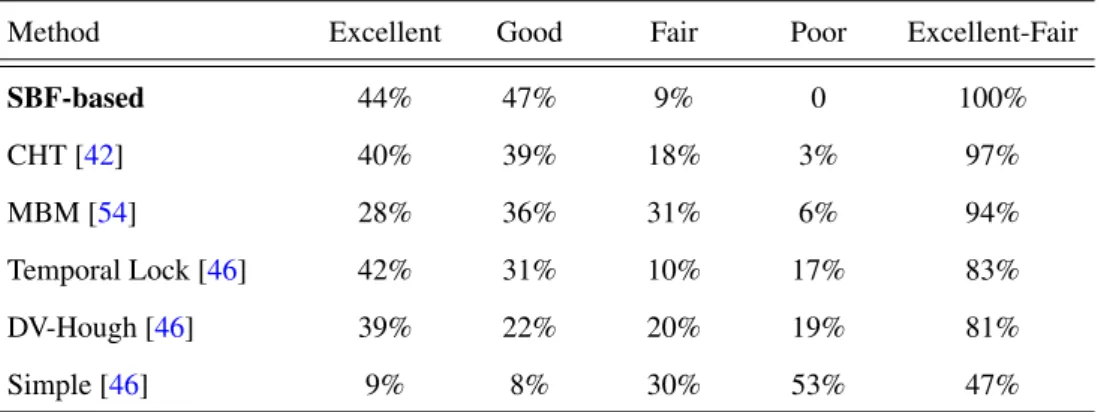
3.9 Comparison between proposed SBF-based method and four other methods in terms of percentage images per subjective category (ONHSD). . . 47

(20)

3.10 Samples of OD segmentation in the ONHSD (solid line: results of proposed method, dots: mean of clinician boundaries). (a) Excellent (δ =0.5); (b) Good

(δ =1.4); (c) Fair (δ =2.3). . . 48

3.11 Comparison between the SBF-based method and other methods in terms of per-centage of images per overlapping interval (MESSIDOR dataset). . . 49

3.12 Samples of OD segmentation in MESSIDOR dataset (Dashed line: results of pro-posed method, Solid line: manually extracted boundaries by experts). (a)S=0.97; (b)S=0.86; (c)S=0.78. . . 49

3.13 Samples of OD segmentation in the presence of exudates, peripapillary atrophy and blurredness; (a) DR: D3 and ME: R2; (b) DR: D3 and ME: R1; (c) DR: D3 and ME: Normal; (d) DR: D1 and ME: Normal ; (e) DR: D3 and ME: Normal; (f) DR: D3 and ME: R2. . . 51

3.14 Samples of OD segmentation in different conditions of contrast and illumination. 52

3.15 OD segmentation in MESSIDOR dataset where the initial OD detection (black cross) failed with the low-resolution ODC location (gray cross) and final ODC location (white cross); (a and b) The method failed to detect and segment the OD (S=0); (c) The method overcame the initial OD localization failure and seg-mented the OD correctly (S=0.90). . . 52

3.16 Samples of OD segmentation in INSPIRE-AVR dataset (Dashed line: results of proposed method, Solid line: manually extracted boundaries by an expert). (a)

S=0.97; (b)S=0.86; (c)S=0.75. . . 53

4.1 Block diagram of the proposed method for A/V classification. . . 57

4.2 Graph generation. (a) Original image; (b) Vessel segmentation image; (c) Center-line image; (d) Extracted graph. . . 58

4.3 Graph Modifications. (a), (d), (g) Typical errors; (b), (e), (e) Graph representation of the worst-case scenarios; (c), (f), (i) Final graph after modification. . . 60

(21)

LIST OF FIGURES xvii

4.5 (a)-(c) Possible configurations for nodes of degree 2; (d)-(f) Possible configura-tions for nodes of degree 3. . . 64

4.6 (a)-(c) Possible configurations for nodes of degree 4; (d) Node of degree 5. . . 66

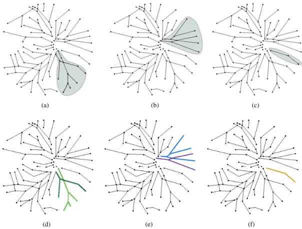
4.7 Examples of subgraph labeling where each color represent a distinct label; (a) Paired subgraph 1; (b) Paired subgraph 2; (c) Unpaired subgraph 3; (e), (e) and (f) Results of link labeling in subgraphs (a), (b) and (c). . . 68

4.8 (a) Separate subgraphs (b) Final result of graph analysis. . . 68

4.9 Examples of assigning A/V classes to the labels in each subgraph using LDA classifier; (a), (d) and (g) Graph analysis results for each subgraph; (b), (e) and (h) LDA classifier result; (c), (f) and (i) Final result of assigning A/V classes. . . 71

4.10 (a) LDA classifier result; (b) Final result of supervised graph-based A/V classifi-cation; (c) A/V classification result overlapped on original image (Red: arteries, Blue: veins). . . 71

4.11 Histograms and normal distribution fits for artery and vein pixels based on manual A/V classification in (a) Red channel; (b) Green channel; (c) Blue channel; (d) Hue; (e) Saturation; (f) Intensity. . . 72

4.12 (a) Original image; (b) Normalized red plane; (c) Intensity of vessel pixels. . . . 73

4.13 Initial cluster centroid positions on the sorted set of intensities. . . 74

4.14 Initial cluster centroid positions on the histogram of Red intensity. . . 74

4.15 (a)k-means clustering result (Red: artery, Blue: vein and Green: unknown); (b)

Paired subgraphs; (c) Result of assigning A/V classes to paired subgraphs using

k-means algorithm. . . 74

(22)

4.17 Samples of A/V classification results in INSPIRE-AVR dataset (Red: correctly classified arteries, Blue: correctly classified veins, Green: wrong classification); (a), (g) Original images; (b), (h) Manual A/V labeling; (c), (i) Supervised A/V classification results (accuracy = 97.7% and 61.2%); (d), (j) Comparison of su-pervised A/V classification results with manual labeling; (e), (k) Unsusu-pervised A/V classification results; (f), (l) Comparison of unsupervised A/V classification results with manual labeling (accuracy = 89.6% and 70.1%). . . 77

4.18 Accuracy of correctly classified vessel pixels for the supervised and unsupervised approaches in entire image and inside the ROI. . . 79

4.19 Performance of the supervised graph-based method (Red dot) and unsupervised approach (Yellow dot) compared with the results of Niemeijer’s method (Blue dot: best cut-off, Purple dot: sensitivity cut-off and Green dot: specificity cut-off); (a) INSPIRE-AVR dataset; (b) DRIVE dataset. . . 80

4.20 Samples of A/V classification results in DRIVE dataset (Red: correctly classified arteries, Blue: correctly classified veins, Green: wrong classification); (a), (g) Original images; (b), (h) Manual A/V labeling; (c), (i) Supervised A/V classifi-cation results (accuracy = 96.1% and 72.9%); (d), (j) Comparison of supervised A/V classification results with manual labeling; (e), (k) Unsupervised A/V classi-fication results; (f), (l) Comparison of unsupervised A/V classiclassi-fication results with manual labeling (accuracy = 88.8% and 78.5%). . . 82

4.21 Samples of A/V classification results in CHSJ dataset (Red: correctly classified arteries, Blue: correctly classified veins, Green: wrong classification); (a), (g) Original images; (b), (h) Manual A/V labeling; (c), (i) Supervised A/V classifi-cation results (accuracy = 83.5% and 84.2%); (d), (j) Comparison of supervised A/V classification results with manual labeling; (e), (k) Unsupervised A/V classi-fication results; (f), (l) Comparison of unsupervised A/V classiclassi-fication results with manual labeling (accuracy = 92.5% and 93.1%). . . 83

5.1 Block diagram of the proposed method for AVR estimation. . . 88

(23)

LIST OF FIGURES xix

5.3 (a) Retinal image with the ODC (black cross) detected using the method based on the entropy of vascular directions; (b) Circular OD boundary using a fixed OD radius of 180 pixels centered on the initial ODC in (a); (c) ROI for AVR calculation (delimited by the two green circles) with a fixed OD radius; (d) OD boundary using SBF-based method; (e) Approximation of the OD boundary by a circle (radius of 215 pixels); (f) ROI for AVR calculation (delimited by the two green circles) and the estimated optic disc margin (white circle). . . 91

5.4 (a) A/V classification result using the supervised graph-based method; (b) Main vessels inside the ROI (supervised AV classification and fixed OD radius); (c) A/V classification results using the unsupervised graph-based method; (d) Main vessels inside the ROI (unsupervised AV classification and OD segmentation). . . 93

5.5 Region of interest divided in six concentric regions. . . 94

5.6 Bland-Altman plots of the agreement (a) between Observer 2 and reference; (b) between Niemeijer’s method and reference; (c) between Method 1 and reference; (d) between Method 2 and reference; (e) between Method 3 and reference. . . 96

5.7 Boxplot of AVR values for different methods. . . 99

5.8 Scatter plots and regression lines between reference AVR values (a) between Ob-server 2 and reference; (b) between Niemeijer’s method and reference; (c) be-tween Method 1 and reference; (d) bebe-tween Method 2 and reference; (e) bebe-tween between Method 3 and reference. . . 100

5.9 (a) Number of subjects with matched classification between methods and refer-ence; (b) Number of subjects with mismatched classification between methods and reference . . . 101

6.1 RetinaCAD graphical user interface; (a) Main screen; (b) Second display; (c) Report.105

(24)

6.3 Examples of obtained AVR values and AV classification results inside the ROI for different images of 2 subjects from CHSJ dataset; each column shows the results for each subject; (a), (b) results for right eye with 30° FOV; (c), (d) results for right eye with 45° FOV; (e), (f) results for left eye with 30° FOV; (g), (h) results for left eye with 45° FOV; (Green circles: ROI delimitation, White circle: estimated OD, Red: arteries, Blue: veins). . . 110

6.4 Boxplot of AVR values for different eyes (right and left) and different FOV (45° and 30°). . . 112

6.5 Bland-Altman plots of the agreement between AVR values from the same eye with 45° and 30° FOV for (a) right eyes; (b) left eyes. . . 113

6.6 Bland-Altman plots of the agreement between AVR values from right and left eyes for (a) images with 45° FOV; (b) images with 30° FOV. . . 114

6.7 Scatter plots and regression lines for AVR values of the same eye with 45° and 30° FOV for (a) right eyes; (b) left eyes; and for AVR values from right and left eyes for (c) images with 45° FOV; (d) images with 30° FOV. . . 115

(25)

List of Tables

2.1 The performance of vessel segmentation methods. . . 16

2.2 The performance of optic disc segmentation methods. . . 21

2.3 The performance of A/V classification methods. . . 25

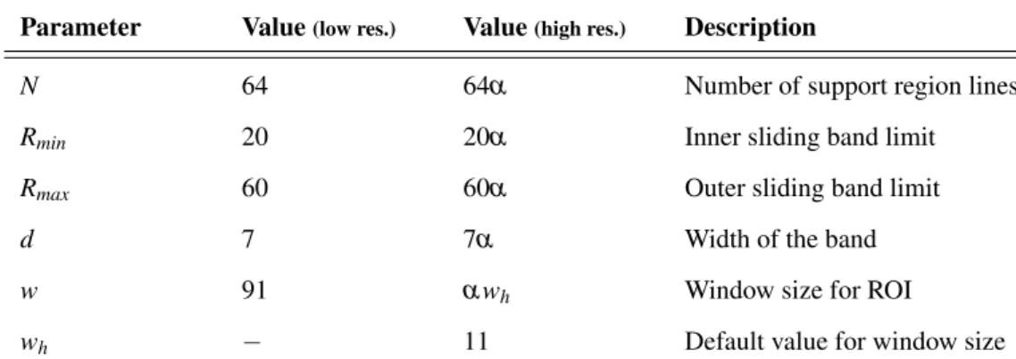
3.1 Parameters setting defined using ONHSD. . . 44

3.2 Parameters setting for low-resolution SBF and high-resolution SBF. . . 45

3.3 Scale factors for different datasets. . . 45

3.4 Parameter settings for high-resolution SBF for MESSIDOR and INSPIRE-AVR datasets. . . 45

3.5 Comparison between proposed SBF-based method and four other methods in terms of percentage images per subjective category (ONHSD). . . 46

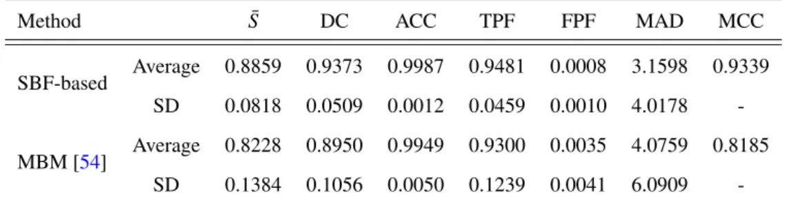
3.6 Comparison of the average and standard deviation of different measures between proposed method and MBM on ONHSD dataset. . . 47

3.7 Comparison between the SBF-based method and other methods in terms of per-centage of images per overlapping interval and average overlapping of the whole set (MESSIDOR dataset). . . 49

3.8 Comparison of the average and standard deviation (SD) of different measures be-tween proposed method and MBM on MESSIDOR dataset. . . 50

3.9 Comparison between SBF-based method and F-HLSM method in terms of per-centage images per subjective category based on the ratio between MAD and esti-mated OD radius (MESSIDOR dataset). . . 50

3.10 The average (standard deviation) of overlapping score (S) for the images of MES-SIDOR dataset with different DR and ME grades. . . 53

(26)

3.11 The average and standard deviation of different measures on INSPIRE-AVR dataset. 53

4.1 Graph Notations. . . 59

4.2 Different cases of nodes and the possible node types. . . 63

4.3 List of features measured for each centerline pixel. . . 69

4.4 Performance evaluation and comparison of individual intensity-based classifiers (INSPIRE-AVR dataset). . . 70

4.5 Accuracy of individual methods before and after combination (INSPIRE-AVR dataset). . . 78

4.6 Supervised graph-based method: accuracy rates for the entire image and inside the ROI (INSPIRE-AVR dataset). . . 78

4.7 Unsupervised graph-based method: accuracy rates for the entire image and inside the ROI (INSPIRE-AVR dataset). . . 78

4.8 Comparison of sensitivity and specificity values . . . 80

4.9 Accuracy of correctly classified pixels using supervised and unsupervised graph-based approaches for the main vessels. . . 81

5.1 AVR values for the 40 images of the INSPIRE-AVR dataset . . . 97

5.2 AVR values for the 40 images of the INSPIRE-AVR dataset . . . 98

6.1 Comparison of Mean ± SD (Min - Max) of measurements for different eyes (right and left) and different FOV (45° and 30°). . . 111

6.2 Comparison of Mean ± SD (Min - Max) of measurements for different eyes (right and left) with both FOVs of 45° and 30° and different FOVs (45° and 30°) for both right and left eyes. . . 111

6.3 Comparison of AVR values between images of the same eye with 45° and 30° FOV.112

6.4 Comparison of AVR values between images right and left eyes. . . 113

6.5 Average of AVR values and 95% confidence intervals for the subjects with differ-ent pathological conditions. . . 117

(27)

Abbreviations and Symbols

A/V Artery/Vein

ACC Accuracy

AUC Area Under Curve

AVR Arteriolar-to-Venular Ratio

BP Blood Pressure

CAD Computer-Aided Diagnosis

CRAE Central Retinal Artery Equivalent

CRVE Central Retinal Venular Equivalent

DC Dice’s coefficient

DR Diabetic Retinopathy

FOV Field of View

FPF False Positive Fraction

LDA Linear Discriminant Analysis

MAD Mean Absolute Distance

MCC Matthews Correlation Coefficient

ME Macular Edema

OD Optic Disc

ODC Optic Disc Center

RetinaCAD Retinal Computer-Aided Diagnosis

ROI Region of Interest

ROC Receiver Operating Characteristic

SBF Sliding Band Filter

TPF True Positive Fraction

(28)

(29)

Chapter 1

Introduction

The retina is the only part of the human body where the blood circulation can be observed di-rectly. Several systemic diseases can affect the retinal blood vessels, which makes the retinal image analysis a potential diagnostic tool, as it allows assessing vascular changes in an easy and non-invasive way. Retinal image analysis is one of the active research areas with the goal of providing computer-aided methods to help the quantification, measurement and visualization of retinal landmarks and biomarkers.

In diabetic retinopathy (DR), the blood vessels often show abnormalities at early stages [1], as well as vessel diameter alterations [2]. Changes in retinal blood vessels, such as significant dilatation and elongation of main arteries, veins, and their branches [2,3], are also frequently associated with hypertension and other cardiovascular pathologies.

The greatest emphasis in automated diagnosis has been given to the detection of diabetic retinopathy. Diabetes is reaching epidemic proportions worldwide, due to the growth of popu-lation, urbanization and increasing adult obesity prevalence and physical inactivity. The recent report by the International Diabetes federation (IDF) [4] indicates that 8.3% of adults (387 million people) have diabetes, and the number of people with the disease is set to rise beyond 592 million by 2035. Yet, with 175 million of cases currently undiagnosed, a vast amount of people with di-abetes are progressing towards complications unawares. People with didi-abetes have an increased risk of developing a number of serious health problems. Consistently high blood glucose levels can lead to serious diseases affecting the heart, the blood vessels, eyes, kidneys and nerves. In addition, people with diabetes also have a higher risk of developing infections, which can cause blindness, kidney failure, lower limb amputation, stroke and sudden death. In 2014 diabetes was the direct cause of 4.9 million deaths.

(30)

Diabetic retinopathy is divided into various stages based on severity. The early signs like microaneurysms, hemorrhages and cotton wool spots are known as non-proliferative diabetic retinopathy [1]. Proliferative diabetic retinopathy develops from occluded capillaries that lead to retinal ischemia and formation of new vessels on the surface of the retina near the optic disc (OD). Certain lesions, such as the number of microaneurysms and dot hemorrhages correlate with sever-ity and progression of the diseases [5]. Retinal vessel dilatation is a well-known phenomenon in diabetes and significant dilatation and elongation of arterioles, venules, and their macular branches occur in the development of diabetic macular edema that can be linked to hydrostatic pressure changes [6].

The World Health Organization (WHO) [7] rates hypertension as one of the most important causes of premature death worldwide and the problem is growing. There are at least 970 million people worldwide who have elevated blood pressure (hypertension) and in 2025 it is estimated there will be 1.56 billion adults living with high blood pressure. Hypertension is a major risk factor for coronary heart disease and ischemic as well as hemorrhagic stroke. Blood pressure levels have shown to be positively and continuously related to the risk for stroke and coronary heart disease. High blood pressure is called the “silent killer" since it often has no warning signs or symptoms, and many people do not realize they have it. Hypertension can cause changes to the retina, such as localized or generalized narrowing of vessels, copper wiring and silver wiring, arteriovenous nicking, hemorrhages, nerve fiber layer losses, increased vascular tortuosity, cotton wool spots and exudates [1].

For both diseases, the early diagnosis of diabetes and hypertension are crucial to prevent and reduce the pathological damages, which can be achieved through the use of retinal image analy-sis. Detection of lesions or vessel changes and measurement of useful objective and reproducible health indicators can improve the capability of early diagnosis.

1.1 Motivation

Current techniques for the assessment of vascular changes in retinal images are mostly semi-automated or manual which require trained experts to help the process by searching large numbers of retinal images. The application of digital imaging to ophthalmology has now provided the possibility of automated analysis of retinal images to assist clinical diagnosis and treatment.

(31)

1.2 Contributions 3

than current observation techniques. Advantages in a clinical context include the potential to per-form automated screening for conditions such as diabetic retinopathy, and hence to reduce the workload required from manual trained graders.

However, even in healthy retinal images, the automatic detection of retinal landmarks and features requires varied and innovative image processing, image analysis and machine learning techniques. In retinal images with pathology, there is wider field of patterns and features to target, and it is also a challenging task to develop robust and reliable algorithms in the presence of patho-logical conditions. Researchers and experts in pattern recognition and image analysis find retinal images exciting, challenging, and rewarding to work with. There are quite a number of problems in automated retinal analysis that need to be solved before the computer-aided diagnosis systems can be used for general clinical applications.

This work is mostly focused on the development of retinal image analysis techniques for the automatic assessment of vascular changes caused by systemic diseases. Within this context, some of the challenges are being able to accurately segment the vessels, measure the vessel caliber, extract the OD boundary and classify the blood vessels as arteries or veins. The location and radius of OD and the artery/vein (A/V) classification are required as prerequisite stages for calculating important vascular signs, which can provide clinically valuable information to aid prevention and management of diseases namely diabetes and hypertension.

1.2 Contributions

The aims of the work presented in this thesis are the development of algorithms and tools for the retinal image analysis allowing an automatic and reproducible assessment of retinal vascular changes. The starting point of this work is based on a vessel segmentation method previously developed by our research group [8]. The main contributions of this thesis can be summarized as follows:

•A fully automatic method which segments the optic disc independently of image

(32)

•A fully automatic method which classifies the vessels as arteries or veins based on a graph

extracted from a vascular tree. This method is able to classify the whole vascular tree and does not restrict the classification to specific regions of interest. While most of the recent methods mainly use intensity features for discriminating between arteries and veins, the proposed method uses additional information extracted from a graph which represents the vascular network. The promising results of the proposed graph-based A/V classification method on the images of three different datasets demonstrate the independence of this method with various properties, such as differences in size, quality, and camera field of view [10].

•Automatic approaches for calculating the Central Retinal Artery Equivalent (CRAE),

Cen-tral Retinal Venular Equivalent (CRVE) and Arteriolar-to-Venular Ratio (AVR) in retinal images which are supported by a new approach for optic disc segmentation and by new supervised and unsupervised techniques for A/V classification. These methods are evaluated on a public dataset, where the mean error of the measured AVR values with respect to the reference was identical to the one achieved by a medical expert using a semi-automated system, thus demonstrating the reliability of the proposed methods for AVR estimation [11,12].

•RetinaCAD, a user-friendly retinal computer-aided diagnosis system, that is able to automat-ically detect, measure and classify two main retinal landmarks, the optic disc and the vessels. Reti-naCAD can measure several vascular features that are recognized as indicators for some prevalent systemic diseases, namely CRAE, CRVE and AVR, as well as various geometrical features associ-ated with vessel bifurcations. This application was assessed in the images of a new dataset from a local hospital, where it showed an association between AVR values and clinical information. The lower AVR values in the subjects with pathological conditions in contrast to the non-pathological ones demonstrates the potential of the system as a CAD tool for early detection and follow-up of diabetes, hypertension or cardiovascular pathologies [13].

(33)

1.3 Organizational Overview 5

1.3 Organizational Overview

Together with this chapter, the research reported in this Ph.D. thesis is organized in the following chapters.

Chapter2provides a general literature review on retinal image analysis methods useful for the assessment of vascular changes, namely vessel segmentation, optic disc detection, A/V classifica-tion and assessment of vascular changes.

Chapter3introduces an automatic approach for optic disc segmentation using a multiresolu-tion sliding band filter (SBF).

Chapter4presents an automatic artery/vein classification method based on the analysis of a graph extracted from the retinal vasculature. Final classification of a vessel segment as A/V is performed by means of supervised and unsupervised approaches.

Chapter5is devoted to the presentation of approaches for the automated assessment of vascu-lar changes, particuvascu-larly the measurement of CRAE, CRVE and AVR indexes.

Chapter 6 presents RetinaCAD (Retinal Computer-aided Diagnosis System) and shows the results of the proposed system evaluation as well as the clinical validation.

(34)

(35)

Chapter 2

Retinal Image Analysis for the

Assessment of Vascular Changes.

Overview

Retina is a light-sensitive tissue lining the inner surface of the eye (Figure 2.1(a)). When an ophthalmologist uses an ophthalmoscope to look into the eye he sees a retinal image like the one in Figure2.1(b). In the center of the retina is the optic disc which is the beginning of the optic nerve and the entry point for the major blood vessels that supply the retina. Fovea can be seen in Figure2.1(b)as the blood vessel-free reddish spot, in the center of the area known as the macula. The blood vessels of the retina radiate from the center of the optic disc. The walls of the retinal blood vessels are transparent and therefore the column of blood flowing in these vessels can be directly observed. The arteries appear lighter and narrower when compared to the veins. Retina is the only part of blood circulation system that can be observed directly, so any vascular changes or abnormality can be detected and can be used for screening.

Some of the pathologies that affect the retina are age-related macular degeneration, glaucoma, retinopathy of prematurity, diabetic retinopathy and hypertension [14]. Some of these diseases are now amenable to automated identification and assessment. In addition, retinal blood vessel pattern can also provide information on the presence or risk of developing hypertension, diabetes, cardiovascular or cerebrovascular diseases [14].

The retinal vasculature can be observed directly and it is easily accessible to study the health of the human microcirculation in vivo. Pathological changes of the retinal vasculature, such as the appearance of microaneurysms, focal areas of arteriolar narrowing, arteriovenous nicking, and

(36)

retinal hemorrhages are common fundus findings in older people, even in those without hyper-tension or diabetes. Recent advances in retinal image analysis have allowed reliable and precise assessment of these retinal vascular changes, as well as objective measurement of other topo-graphic vascular characteristics such as retinal vascular widths, geometrical attributes at vessel bifurcations and vessel tracking.

(a) (b)

Figure 2.1: The retina (a) Eye anatomy; (b) Retinal image.

In this chapter, the principles of retinal digital image analysis and the techniques for extract-ing the signs related to the retinal vascular changes are discussed. The methods for detectextract-ing and classifying the main retinal landmarks are critical components of circulatory blood vessel analysis systems, so it would be valuable to start with reviewing the methods for retinal vessel segmen-tation, optic disc segmentation and artery/vein (A/V) classification (in Sections2.1,2.2and2.3). After that the methods for extracting the signs related to the retinal vascular changes are described in Section2.4. Finally, Section2.5summarizes the concluding remarks.

2.1 Vessel Segmentation

(37)

2.1 Vessel Segmentation 9

Most of the vessel segmentation methods utilise the contrast existing between the retinal blood vessel and surrounding background. However, there are several challenges in retinal vessel seg-mentation that makes it a non-trivial task. There are other structures in the image such as the retina boundary, the optic disc, and bright or dark spots (caused by pathologies) which can negatively influence the process of vessel segmentation. On the other hand, the narrow vessels have a very low contrast in comparison with the background which makes the discrimination even harder. In addition, the effect of central reflex in wider vessels makes it complex to distinguish one vessel from two side-by-side vessels.

Vessel segmentation algorithms and methods can be divided into three main categories [15,16]: image analysis approaches, tracking-based approaches and classification-based approaches.

2.1.1 Image Analysis Approaches

Image analysis approaches extract meaningful information from images and use that information for segmenting the vessels. These image analysis approaches can be organized into four categories: multi-scale approaches, centerline detection methods, region growing approaches and matched filters approaches [15,16].

Multi-scale approaches perform segmentation on different image resolutions. Thick vessels

are extracted at low resolution images and then thinner structures, such as deriving branches of already segmented structures, can be segmented at higher resolution. The main advantages of this technique are the increased processing speed and the increased robustness. Qin Li et al. [17]

proposed a vessel segmentation method which includes a multi-scale analytical scheme using Gabor filters and scales multiplication. Scale multiplication, which is defined as the product of Gabor filter responses at two adjacent scales, enhances the edges and filters noise. After that they use a threshold probing technique utilizing the features of the retinal vessel network which uses a line tracking algorithm to guide the selection of the threshold. Lathenet al.[18] accomplish vessel

(38)

Moghimiradet al. [19] present a multi-scale approach based on a weighted 2D medialness

function. The result of the medialness function is first multiplied by the eigenvalues of the Hessian matrix in every pixel of the image in order to extract vessel’s medial-lines. After that, by extracting the centerlines of vessels and estimation of radius of vessels, the retinal vessels are segmented. Li

et al.[20] used the multi-scale production of multi-scale matched filters for vessel segmentation.

The scale production is used to enhance the edges and decrease noise so that some small weak vessels with low local contrast are detected with good width estimation. Saffarzadeh et al.[21]

proposed a vessel segmentation technique based on a multi-scale line detection. This method uses a perceptive transform based on Weber’s law, and then reduces the impact of bright lesions by

k-means clustering. Afterwards, a line operator is used in three scales for the vessels detection and

the segmentation is finalized by thresholding to ignore some of the dark lesions.

Centerline detection approachesextract blood vessel centerline segments then create the

ves-sel tree by connecting these centerline segments. Different approaches are used to extract the centerline structure. Mendonçaet al.[8] proposed an algorithm which starts with the extraction

of vessel centerlines by using directional information from a set of four directional Difference-of-Offset-Gaussians filters. After that, a region growing process guided by some image statistics connects the candidate points. The final segmentation is obtained using an iterative region grow-ing that integrates the contents of several binary images resultgrow-ing from vessel width dependent morphological filters. Recently, Mendonçaet al. extended their method for segmenting high

res-olution images [22]. Wuet al.[23] describe a segmentation approach for vessel centerlines based

on ridge descriptors. The proposed ridge descriptor contains the normalized largest curvature and the orientations of gradients in the local neighborhood. For vessels of a certain scale, the distribu-tion of the descriptors is assumed to have a normal distribudistribu-tion estimated from a training set with known ground truth. Then vessel center line segmentation can be performed based on the distance between the ridge descriptor at candidate pixels and the learned model.

Region growing approachesselect a set of seed points based on some predefined criteria. The

initial region begins at the exact location of these seeds. The regions are then grown from these seed points to adjacent points depending on a region membership criterion like same intensity characteristics. Martinez-Perezet al.[24] presented a method based on the scale-space analysis of

(39)

features for a region growing procedure. The growth is constrained to regions of low gradient magnitude and then the borders between regions will be defined by growing vessel and background classes without gradient restriction.

Graget al.[25] described an unsupervised, curvature-based method for segmenting the

com-plete vessel tree from color retinal images. The vessels are modelled as trenches and the medial lines of the trenches are extracted using the curvature information derived from a curvature esti-mate. After that, the vessel structure is extracted using a modified region growing method, where the medial points detected by the trench detection algorithm serve as seed points. The region is grown only around a selected neighborhood of the seed point, whose size is based on the width of the largest vessel.

Matched filters approaches convolve the image with multiple matched filters for extracting

objects of interest, as in Sofkaet al.[26] for extracting vessels in retinal images. The core of the

technique is a new likelihood ratio test that combines matched filter responses, confidence and vessel boundary measures. Matched filter responses are derived in scale-space to extract vessels of widely varying widths. Vessel boundary measures and associated confidences are computed at potential vessel boundaries. The combination of these responses forms a six-dimensional mea-surement vector at each pixel. A training technique is used to develop a mapping of this vector to a likelihood ratio that measures the vesselness at each pixel. Finally, the new vesselness likelihood ratio is embedded into a vessel tracing framework for vessel centerline extraction.

The method proposed by Ramlugunet al. [27] segments the blood vessels using an 2-D

Ga-bor filter on a histogram-equalized image followed by hysteresis thresholding. Fathiet al.[28]

presents a method based on complex continuous wavelet analysis to enhance blood vessels and to remove noise. The segmented vessels are obtained by an adaptive histogram-based threshold-ing procedure along with proper length filterthreshold-ing process. Krause et al.[29] porposed a vessel

segmentation method based on the local Radon transform for the vessel smoothing. This method first enhances the contrast of blood vessels using a second-order differential operator, and then the vessels are detected by the combination of smoothing along vessel directions with contrast enhancement across them.

2.1.2 Tracking-based Approaches

(40)

by analyzing the pixels orthogonal to the tracking direction. Different methods are employed for determining vessel contours or centerlines. An advantage of tracking based methods is the connectedness of vessel segments, which is not guaranteed in pixel processing based methods.

Vlachoset al.[30] proposed an algorithm for vessel segmentation and network extraction in

retinal images. In this method, a new multi-scale line-tracking procedure starts from a small group of pixels, derived from a brightness selection rule, and terminates when a cross-sectional profile condition becomes invalid. The multi-scale image map is derived after combining the individual image maps along scales, containing the pixels confidence to belong to a vessel. The initial vessel network is derived after map quantization of the multi-scale confidence matrix. Median filtering is applied in the initial vessel network, restoring disconnected vessel lines and eliminating noisy lines. In the final step, post-processing removes erroneous areas using directional attributes of vessels and morphological reconstruction. Niemeijer et al. [31] proposed an automated vessel

linking framework that connects together separate pieces of the retinal vasculature into a connected vascular tree. To determine which vessel sections should be linked together they use a supervised cost function.

Yinet al. [32] presented a probabilistic tracking method for the blood vessel detection. In

the tracking process, vessel edge points are detected iteratively using local gray-level statistics and vessel continuity properties. A Gaussian-shaped curve is used for estimating the local vessel sectional intensity profiles. Local vessel structure and the edge points are obtained by means of a Bayesian method with the maximum a posteriori probability criterion. Bekkerset al.[33] proposed

two vessel edge tracking algorithms which are based on an orientation score. These algorithms use invertible and non-invertible orientation scores by means of cake wavelets and Gabor wavelets. They also presented a fast method for vessel centerline tracking through a multi-scale set of non-invertible orientation scores where the multi-scale approach makes the algorithm less stable at crossings and bifurcation points.

2.1.3 Classification-based Approaches

Classification-based approaches aim at finding hypotheses that explain the training data and use these hypotheses for classifying each pixel as vessel or non-vessel. Niemeijeret al.[34] extract a

(41)

based on the extraction of image ridges (expected to coincide with vessel centerlines) used as primitives for describing linear segments, named line elements. Each pixel is assigned to the nearest line element to form image patches, and then classified using a set of features from the corresponding line and image patch. The feature vectors are classified using a kNN classifier. The feature selection is based on sequential forward feature selection which, in each step, selects the best feature that satisfies some criterion function and includes it in the current feature set. The set that gives the best performance is chosen.

The method presented in [36] by Soares et al. also adopts supervised classification. Each

image pixel is classified as vessel or non-vessel based on the pixel feature vector, which is com-posed of the pixel intensity and 2-D Gabor wavelet transform responses taken at multiple scales. A Gaussian-mixture model classifier (a Bayesian classifier in which each class-conditional proba-bility density function is described as a linear combination of Gaussian functions) is then applied to obtain the final segmentation. Lupascu et al. [37] proposed a method for automated vessel

segmentation in retinal images. For each pixel in the field of view of the image, a 41-D feature vector is constructed. The feature vector consists of the output of filters, vesselness, and ridgeness measures based on eigen decomposition of the Hessian computed at each image pixel, and the output of a 2-D Gabor wavelet transform taken at multiple scales. Moreover, the feature vector includes the principal curvatures, the mean curvature, and the values of principal directions of the intensity surface computed at each pixel of the green component image. The value of the root mean square gradient and the intensity within the green component at each pixel are also included in the feature vector. After that an AdaBoost classifier is trained on gold standard examples of vessel and nonvessel pixels, and then used for classifying previously unseen images.

Neural networks (NN) are used for simulating biological learning and are widely used in ptern recognition mainly for classification. One of the advantages that make neural networks at-tractive in medical image segmentation is their ability to use nonlinear classification boundaries obtained during the training of the network. Another attractive feature of the neural nets is the ability to learn. In this regard, Marinet al.[38] presented a supervised method for blood vessel

(42)

enhanced by the inclusion of a two-step post processing stage: the first step fills pixel gaps in detected blood vessels, while the second step removes isolated vessel pixels.

Franklinet al.[39] proposed a retinal vessel segmentation technique using neural networks. In

the first stage, a Gaussian filter is used to smooth the gray-scale image, then the Gabor features at different orientations and moment invariants-based features are measured. In the next phase, some samples are taken from vessel and nonvessel regions to train the NN. Afterwards each pixel of a retinal image is classified as vessel or nonvessel using a multi-layer perceptron neural network and a back propagation algorithm, which changes the weights in the feed forward network.

Perfettiet al.[40] exploited the geometrical properties of blood vessels by calculating the line

strength of the blood vessels in the green plane of the retinal image. The line strength image was obtained with simple cellular neural network (CNN) templates in a multistep operation with virtual template expansion. The proposed CNN algorithm requires only linear space-invariant 3_×3 templates, so it could be implemented using one of the existing very-large-scale integration chips.

Wanget al.[41] presented a hybrid approach using a convolutional neural network and

en-semble random forests (RFs) for blood vessel segmentation. This method starts by a set of pre-possessing steps to normalize nonuniform illumination and to enhance the vessels contrast. Then a convolutional neural network is used for extracting a set of hierarchical features including multi-scale information about the geometric structure. The convolutional neural network is a supervised feature learner, which is invariant to image translation, scaling and skewing. Afterwards, ensem-ble RFs is trained to obtain a vessel classifier. These ensemensem-ble RFs employ multiple classifiers to obtain better performance by combining the decisions from multiple weak learners.

2.1.4 Vessel Segmentation Evaluation

Most of the retinal vessel segmentation methodologies are evaluated on two publicly available databases, the DRIVE dataset and the STARE dataset, which are introduced in AppendixA. The manual segmentation is provided by two experts for the images of these datasets.

(43)

based on equation (2.2). Specificity is the ability to detect non-vessel pixels using equation (2.3).

ACC= (T P+T N)

(T P+T N+FP+FN) (2.1)

SN= T P

(T P+FN) (2.2)

SP= T N

(FP+T N) (2.3)

where the true positive (T P) is the number of pixels identified as vessel in both the ground truth and

segmented image, and the true negative (T N) is the number of pixels classified as a non-vessel in

the ground truth and the segmented image. False negative (FN) is the number of pixels classified

as non-vessel in the segmented image but as a vessel pixel in the ground truth image, and the false positive (FP) is number of pixels marked as vessel in the segmented image but non-vessel in the

ground truth image.

In addition, the performance of the algorithm can also be measured with the area under the receiver operating characteristic (ROC) curve. The ROC curve is a plot of the true-positive fraction versus the false-positive fraction for different cut-off points of a parameter.

During the literature review, it was observed that some papers describe the performance in terms of accuracy and area under ROC whereas the other articles choose sensitivity and specificity for reporting the performance. As it is shown in Table2.1, the performance of classification-based algorithms is better in general than their counterparts. Almost all the supervised methods report the area under ROC of higher than 0.95 and among them Marinet al.[38] reported the highest.

However, these methods do not work very well on the images with non-uniform illumination as they produce false detection in some images on the border of the optic disc, hemorrhages and other types of pathologies that present strong contrast. Matched filters has been extensively used for automated retinal vessel segmentation [26–29]. Many improvements and modifications are proposed since the introduction of the Gaussian matched filter. The matched filters alone cannot handle vessel segmentation in pathological retinal images; therefore it is often employed in combination with other image processing techniques. The confidence measures and edge measures defined by Sofkaet al.[26] deals with the problem of overlapping of the non-vessel structures like

the retinal boundary and the optic disk in vasculature extraction.

(44)

The main advantage of tracking approaches is the connectedness of vessel segments, which is not guaranteed in other approaches. The classification-based approaches can achieve more accuracy and quality but training these methods is usually computationally more expensive.

Table 2.1: The performance of vessel segmentation methods.

Methods Dataset Sensitivity Specificity Accuracy Area

under ROC

2nd-observer DRIVE 0.7763 0.9723 0.9473

-STARE 0.8951 0.9384 0.9354

-Moghimiradet al.(2012) [19] DRIVE 0.7852 0.9935 0.9659 0.958

STARE 0.7177 0.9753 0.9484 0.9678

Liet al.(2012) [20] DRIVE 0.7154 0.9716 0.9343

-STARE 0.7191 0.9687 0.9407

Saffarzadehet al.(2014) [21] DRIVE - - 0.9387 0.9303

STARE 0.9483 0.9431

Mendonçaet al.(2006) [8] DRIVE 0.7344 0.9764 0.9463

-STARE 0.6996 0.973 0.9479

-Mendonçaet al.(2014) [22] DRIVE 0.7467 0.9762 0.9466

-STARE 0.7194 0.9759 0.9487

-Martinez-Perezet al.(1999) [24] DRIVE 0.7246 0.9655 0.9344

-STARE 0.7506 0.9569 0.941

-Ramlugunet al.(2012) [27] DRIVE 0.6413 0.9767 0.934

-Fathiet al.(2013) [28] DRIVE 0.7768 0.9759 0.9581

-STARE 0.8061 0.9717 0.9591

Krauseet al.(2013) [29] DRIVE - - 0.9468

-Vlachoset al.(2010) [30] DRIVE 0.747 0.955 0.9285

-Niemeijeret al.(2009) [31] DRIVE 0.7145 - 0.9416

-Staalet al.(2004) [35] DRIVE - - 0.9442 0.952

STARE 0.9516 0.9614

Soareset al.(2006) [36] DRIVE - - 0.9466 0.9614

STARE - - 0.948 0.9671

Lupascuet al.(2010) [37] DRIVE 0.72 - 0.9597 0.9561

Perfettiet al.(2007) [40] DRIVE - - 0.9563 0.9558

STARE - - 0.9584 0.9602

Marinet al.(2011) [38] DRIVE - - 0.9452 0.9588

STARE - - 0.9526 0.9769

Wanget al.(2014) [41] DRIVE 0.8173 0.9733 0.9767 0.9475

(45)

2.2 Optic Disc Segmentation 17

2.2 Optic Disc Segmentation

Optic disc is a bright circular shape and all major blood vessels and nerves originate from it. Lo-calization and segmentation of the OD are important tasks in retinal image analysis. The OD shape is an important indicator of many ophthalmic pathologies and also its localization is a prerequisite stage in many retinal image analysis algorithms. Correct segmentation of the OD contour is a non-trivial problem, since the natural variation in the characteristics of the OD is a major difficulty for defining the contour. In addition, blood vessels crossing the OD boundary as well as pathological conditions can negatively influence the OD segmentation process.

There are several works on the automatic segmentation of OD in retinal images which can mainly be grouped into four categories, namely template-based methods [42–45], deformable model methods [46–51], morphological-based approaches [52–54], and pixel classification meth-ods [55,56].

2.2.1 Template-based Methods

Template-based methods obtain the OD boundary approximations by defining a template for OD and using an algorithm which matches the template with different parts of the input image and finds the similarity between them. The matching process moves the template to all possible posi-tions in the image and computes a numerical index that indicates how well the template matches the image in that position. Template-based techniques are flexible and relatively straightforward to use, which makes them one of the most popular approaches for OD detection. Their applica-bility is limited mostly by the available computational power, as identification of big and complex templates can be time-consuming.

In this category, Aquinoet al.[42] follow a voting-type algorithm among three independent

detection methods to locate a pixel within the OD as initial information to define a starting sub-image. Then morphological and edge detection algorithms are applied on the sub-image to seg-ment the OD in the red and green channels separately. In both channels, the OD boundaries are approximated using the Circular Hough Transform (CHT) and finally the one with higher score in the CHT is selected. The method proposed by Wonget al.[43] uses a level-set approach to obtain

the OD boundary, that is afterwards smoothed by fitting an ellipse.

A general energy function proposed by Zhenget al.[44], which integrates priors on the

(46)

cut technique. Recently, Giachetti et al. [45] proposed a multiresolution ellipse fitting method

which combines a radial symmetry detector and a vessel density map to detect the OD in low-resolution image. Afterwards, the OD boundary is determined using refined elliptic contours on the mid-resolution and high-resolution images. The final segmented contour is improved with a snake-based refinement algorithm.

2.2.2 Deformable Model Methods

Deformable models methods try to delineate the optic disc as close as possible. These methods begin by estimating the OD boundary usinga prioriknowledge about the location, size and shape

of OD, then this estimate is modified iteratively using optimization techniques for minimizing defined energy terms. Deformable models methods are autonomous and self-adapting in search for a minimal energy state and they are relatively insensitive to noise and other ambiguities in the images. As disadvantage, these methods can stuck in local minima states and their accuracies are dependent on the convergence criteria used in the energy minimization technique. These ap-proaches can be classified into two categories: free-form deformable models, such as snakes, and parametrically deformable models, such as active shape models (ASMs).

Regarding the deformable model approaches, Lowell et al. [46] determine the OD location

by finding the maximum of a correlation filter using a specialized template. Afterwards, the OD is segmented by means of a deformable contour based on a global elliptical model and on local deformation. In the snake model proposed by Xuet al.[47], after each snake deformation, an

un-supervised approach labels the contour points as edge- or uncertain-points. Then the classification result is used to refine the OD boundary before repeating the contour deformation.

Li and Chutatape [48] proposed a method which extracts a point distribution model from the training set using several landmarks on OD boundaries and on main vessels inside the OD. Then a modified active shape model is used by an iterative matching algorithm to locate the OD and refine the disk boundary. Joshiet al.[49] modified a region-based active contour model. They improved

the Chan–Vese model by using local red channel intensities and two texture feature spaces in the neighborhood of the pixels under analysis.

(47)

set segmentation method with optimized parameters is used which combines the region informa-tion and local edge vector to drive the deformable contour converging to the true OD boundary. In the method proposed by Hsiaoet al.[51], the Canny edge detector and the Hough transform

are used for obtaining the edge map. Afterwards, the edge map is used as an initial contour in supervised gradient vector flow snake which consists of a snake deformation stage and a contour supervised classification stage.

2.2.3 Morphological-based Approaches

Morphological-based methods extract the OD boundary with a set of non-linear operators that act on images by using structuring elements. Mathematical morphology can extract important shape characteristics and also remove irrelevant information.

In the group of mathematical morphology algorithms for OD segmentation, Reza et al.[52]

threshold the green component in order to obtain a binary image with isolated bright parts. Then, morphological opening is used to detect the connected components and to remove the small ones. Afterwards, extended maxima operator and minima imposition are used for extracting the OD and exudate boundaries. In [53], an adaptive mathematical morphology approach is used in two stages. In the first stage a coarse detection of OD boundary is obtained and in the second stage the results are improved. The method described in [54] uses principal component analysis in the first stage to obtain a grey image with an improved representation of the OD. After removing the vessels, a variant of watershed and stochastic watershed are applied. Finally, a geodesic transformation is used to discriminate the watershed regions as OD or non-OD regions.

2.2.4 Pixel Classification Methods

Pixel classification methods are machine learning techniques that can be used to assign a class to the pixels in an image as OD region or non-OD region. Pixel-based classification methods use various features such as intensity, texture from each pixel and its surroundings to find the optic disc. One of the advantages of a pixel classification method is that it avoids the potentially much larger bias in other categories where methods use only one or two feature detectors. On the other hand, one of the limitations in supervised pixel classification methods is that these methods require a training phase, in an always limited training set.

In the pixel-based classification category, Abràmoffet al.[55] proposed a method where 253

(48)

from hue, saturation, brightness space and also the variance in the red, green, and blue channels in a small region around the pixel. Then the most discriminant features (12 features) are selected using a sequential forward-floating search and finally each pixel is classified into rim, cup, or background using the set of selected features and a k-nearest neighbor classifier.

Recently, Chenget al.[56] proposed a method which classifies each superpixel as disc or

non-disc region using histograms with enhanced contrast and texture features. Superpixels are local and coherent regions that provide local image information. The authors used the simple linear iterative clustering (SLIC) algorithm to aggregate nearby pixels into superpixel. Afterwards, superpixel classification is used for initialization of the disc boundary followed by a deformable model for getting the final contour.

2.2.5 Optic Disc Segmentation Evaluation

Most of the optic disc segmentation methods are evaluated on two publicly available databases, the ONHSD and MESSIDOR datasets, which are described in AppendixA. The OD regions are man-ually delineated by experts for the images of these datasets. Table2.2shows the performance of some of mentioned OD segmentation methods. The OD segmentation performance on the MES-SIDOR dataset is evaluated based on the average of overlapping score ( ¯S) [42]. The overlapping

score (S) measures the common area between the OD region obtained using the automatic method

(A) and the region delimited by experts (E), being defined by

S=Area(A∩E)

Area(A_∪E) (2.4)

In ONHSD dataset four clinicians marked 24 OD boundary points and the methods are com-pared by the percentage of images in the excellent-fair category using a discrepancy value [46]. The discrepancy,δjon image jis defined by

δj=

∑

i

m_ij₋µ_ij

σ_ij+ε (2.5)

where µ_ij andσ_ij are, respectively, the mean and standard deviation of values obtained by four clinicians on spokeiof image j,m_ijis the location of the boundary using the segmentation method

(49)

As shown in Table 2.2, the template-based method by Aquino et al.[42] reports the highest

percentage of images in the Excellent-Fair subjective category, while both Chenget al. [56] and

Giachettiet al.(2014) [45] obtained the average of overlapping score equal to 0.88 on the images

of MESSIDOR dataset.

Both the template-based and deformable model methods are based on the edge characteristics. The performance of these methods very much depends on the differentiation of edges from the disc and other structures. The template-based approaches are usually more robust to color, contrast and illumination variations and have better performance in the presence of severe pathological conditions when compared to the methods in other categories.

Table 2.2: The performance of optic disc segmentation methods.

Methods Dataset S¯ Excellent-Fair

subjective category

Aquinoet al.(2010) [42] ONHSD - 97%

MESSIDOR - 86%

Giachettiet al. (2014) [45] MESSIDOR 0.88

-"Simple" Lowelet al.(2004) [46] ONHSD - 47%

"DV-Hough" Lowelet al.(2004) [46] ONHSD - 81%

"Temporal Lock" Lowelet al.(2004) [46] ONHSD - 83%

Yuet al.(2007) [50] MESSIDOR 0.84

-Moraleset al.(2013) [54] ONHSD 0.80

-MESSIDOR 0.82

-Chenget al.(2014) [56] MESSIDOR 0.88

-¯

(50)

2.3 Artery/Vein Classification

Retinal blood vessel classification into arteries and veins is a necessary phase for the automatic detection of vascular changes, and for the calculation of characteristic signs associated with sys-temic diseases. Several methods have been proposed for the A/V classification [57–71] based on different visual and geometrical features which are used for the discrimination between veins and arteries. Arteries are bright red while veins are darker, and in general artery calibers are smaller than vein calibers. Vessel caliber can be affected by diseases, therefore this is not a reliable feature for A/V classification. Arteries also have thicker walls, which reflect the light as a shiny central reflex strip [72]. Another characteristic of the retinal vessel tree is that, at least in the region near the optic disc (OD), veins rarely cross veins and arteries rarely cross arteries, but both types can bifurcate to narrower vessels, and veins and arteries can cross each other [72]. For this reason, tracking of arteries and veins in the vascular tree is possible, and has been used in some methods to analyze the vessel tree and classify the vessels [57–60].

A semi-automatic method for analyzing retinal vascular trees was proposed by Martinez-Perez

et al. in [57], using geometrical and topological properties of single vessel segments and subtrees.

First, the skeleton is extracted from the segmentation result, and significant points are detected. For the labeling, the user should point to the root segment of the tree to be tracked, and the algorithm will search for its unique terminal points and in the end, decide if the segment is an artery or a vein. Another method similar to this was proposed by Rothauset al.[58], which describes a

rule-based algorithm to propagate the vessel labels as either artery or vein throughout the vascular tree. This method uses existing vessel segmentation results, and some manually-labeled starting vessel segments.

Lauet al.[59] constructed their graph over a restricted region of interest around the optic disc

and then assigned the vessel labels by finding the optimal forest in the subgraphs. Joshiet al.[60]

first separated their vascular graph using Dijkstra’s shortest-path algorithm to find different sub-graphs. They then labeled each subgraph as either artery or vein using a fuzzy C-mean clustering algorithm.

Grisanet al.[61] developed a tracking A/V classification technique that classifies the vessels