Regional Integration and Internal Economic Geography in the Portuguese Case – an update

Carlos Pestana Barros & Nicolas Peypoch

A Comparative Analysis of Productivity Change in Italian and Portuguese Airports

WP 006/2007/DE _________________________________________________________

Nuno Crespo and Maria Paula Fontoura

Regional Integration and Internal Economic Geography in

the Portuguese Case – an update

WP 51/2008/DE/UECE _________________________________________________________

Department of Economics

W

P

School of Economics and Management

Regional Integration and Internal Economic Geography in the

Portuguese Case – an update

Nuno Crespo

and Maria Paula Fontoura

(a) University Institute for Social Sciences, Business Studies and Technology,

Department of Economics, Av. das Forças Armadas, 1649-026 Lisboa, Portugal;

e-mail: nuno.crespo@iscte.pt

(b) ISEG, Technical University of Lisboa, Rua Miguel Lúpi, 20, 1200-781 Lisboa,

Portugal; e-mail: fontoura@iseg.utl.pt

Author for Correspondence:

Maria Paula Fontoura

Rua Miguel Lúpi, 20

1200-781 Lisboa, Portugal

Regional Integration and Internal Economic Geography in the

Portuguese Case – an update

Abstract: The effects of the reduction of international trading costs on the internal

economic geography of each country have been very scarcely studied in empirical

terms. With data for Portugal since its adhesion to the European Union, we analyze

the hypotheses put forward by the new economic geography concerning the evolution

of the spatial concentration of the manufacturing industry as a whole and of each

individual sector. We use four alternative concentration concepts and data

disaggregated both at the level of NUTS III (28 regions) and concelhos (275 regions).

Results show a dispersion of manufacturing industry, in line with Krugman and

Elizondo’s (1996) prediction. Individual sectors show a similar tendency, in contrast

with the theoretical hypothesis.

Keywords: trade liberalization, industrial location, Portugal.

1. Introduction

Analysis of the spatial location of economic activity has attracted a vast interest in

the last fifteen years in the context of the so-called new economic geography (NEG),

based on Krugman’s (1991) pioneering model.2 A large number of studies on this

topic have examined the impact of decreasing cross-border trade barriers and

transaction costs on the international distribution of manufacturing industry within

integrated spaces, with special emphasis on the European Union (EU) space.3 This

analysis may nevertheless mask relevant intra-national spatial effects of the location

dynamics in the integrated economies (Storper et al., 2002), which have remained

under-explored.

Two opposing territorial predictions can be found in the context of the NEG about

the possible effects of trade openness on the internal distribution of manufacturing

industry within a country: sectors either spread out in the country or, alternatively,

they become more geographically concentrated. A natural interest of this type of

analysis comes out by recognizing that concentrating economic activity may

contribute to real divergence, i.e. divergence in real per-capita income levels4, while

structural convergence is expected to help real convergence (Baldwin, 1999). In

addition, it has a connection to regional policy by providing guidance for domestic

adjustment policies aiming to face the variation of foreign market access across

domestic regions.

This paper addresses the relation between trade liberalization and nationwide

spatial adjustments of manufacturing industry in the case of Portugal after adhesion of

this country to the EU in 1986. More precisely, we examine whether in the period

dispersion occurred within the country and to what extent there is a link between trade

openness and the observed pattern of industrial spatial adjustments. Both the

manufacturing industry at the aggregate level (i.e. including all sectors) and each

individual sector will be taken into consideration.5 Relative to previous studies, we

consider additional concepts of spatial concentration as well as a much more

disaggregated data at the regional level.

The period analyzed is particularly appropriate to the purpose of this paper, as the

lapse of time since Portugal became a full member of the EU is sufficiently long to

evaluate the spatial relocation of economic activity. Comparing to other similar

studies for the EU members, another advantage of the period investigated is to include

the post-Single Market, as it is characterized by a deep economic integration of the

markets.

A motivation to study this country case is the fact that, in spite of the EU

orientation of the Portuguese trade (with 68.0% of total exports and 58.9 % of total

imports taking place with the EU market in 1986), the economy had remained rather

closed to foreign trade until its entry into the EU, in contrast with a process of deep

reduction of trade barriers undergone in the following period, and reinforced after

1992 with the cancellation of non-tariff barriers proposed by the Single Market.

In the wake of adhesion to the EU, not only tariffs on trade with EU members

were removed, but also schemes of government authorization for imports, a surcharge

on imports covering all trading partners as well as most quantitative restrictions,

dropped in compliance with the accession rules. Besides, adaptation in respect of the

EU’s common external trade policy was largely expressed in an increasing openness

with regard to products from non-EU countries, particularly in traditional sectors of

The paper is organized as follows. Section 2 presents the theoretical background.

Section 3 analyzes the results of previous empirical evidence on this topic. Section 4

describes the data and discusses the different methodologies which will be used in the

empirical evaluation of the Portuguese case, developed in section 5. Section 6

discusses the possible impact of other factors besides cross-border trade liberalization

on the observed intra-national spatial adjustments of Portuguese manufacturing

industry. Section 7 presents some concluding remarks.

2. Trade openness and the internal economic geography of countries: theoretical

guidelines

In the few existing NEG theoretical contributions related to the impact of falling

trading costs on the internal geography of countries, opposing outcomes may be

found. In a pioneering study on this topic, Krugman and Elizondo (1996) posit

dispersion of manufacturing industry as a whole.6 Conversely, Paluzie (2001), based

on Krugman’s (1991) standard framework, shows that lower international trading

costs is more likely to enhance agglomeration of manufacturing activity. Other

extensions of Krugman’s (1991) model with additional refinements, in general predict

a result in line with that of Paluzie (2001). Nonetheless, it has been already shown

that the relative development level of the trading countries (Alonso-Villar, 2001) and

the way transport and trading costs are modeled (Mansori, 2003; Behrens, 2003;

Behrens et al., 2003) might have a crucial impact on the results obtained.

A main explanation for the difference between predictions with respect to the

implications of trade for regional inequalities has been related to the modelling of the

centrifugal forces that tend to weaken such agglomerations (Crozet and Soubeyran,

2004).

This argument is clearly illustrated when comparing Krugman and Elizondo’s

model (henceforth KE) with respect to Paluzie’s. Both models consider a domestic

country containing two regions, labeled 1 and 2, which opens to trade with the rest of

the world, labeled 0. KE contains only one sector, which exhibits increasing returns to

scale, and it comprises only mobile workers. Paluzie, as in the standard model of

Krugman (1991), assumes a model with two sectors and two production factors:

geographically mobile manufacturing workers, which produce a differentiated good

under monopolistic competition and increasing returns to scale, and immobile

agricultural workers, which produce an homogeneous good under perfect competition

and constant returns to scale. There are transport costs both between the internal

regions, labeled τ, and between the latter and the rest of the world, labeled η, being

the transport cost equal from any of the regions to 0 (η1,0 = η2,0). Transport costs are

modeled with the iceberg approach, which assumes that the cost of transporting a

good uses up only some fraction of the good itself, rather than using any other

resources. They include not only physical transport costs, related to infrastructures,

transport means and distance, but also barriers to trade.

The centripetal forces are represented in both models by backward and forward

linkages, which express the fact that firms and consumers are interested in locating in

the same region. Trade liberalization decreases these agglomeration forces as

progressively more inputs are sourced from abroad and more output is sold in the

exterior market, thus lowering the incentive for domestic firms to locate near other

The main difference between the two models lies in the repellent forces. In KE

they are created by diseconomies associated to agglomerations such as congestion and

high land costs and rents. As trading costs decrease significantly and the centripetal

forces are diluted, firms tend to move away from the more congested region (where

the centrifugal force is stronger) to the other region, in order to benefit from lower

wages and rents. Through numerical simulations, KE observe that with an

intermediate value for η there are several stable equilibria: a symmetric equilibrium in

which the manufacturing industry is evenly divided between the two domestic regions

or, alternatively, a concentration in one of the regions. However, when η is low

enough, the only stable equilibrium is the symmetric distribution. The opening of

trade may therefore lead to a dispersal of manufacturing industry across the country.

We designate this hypothesis as [H1].

Yet, Paluzie, by assuming the immobility of agricultural inputs in opposition to

those of manufacturing, replaces the centrifugal force of large commuting costs and

land rents by the pull of the potential market of a dispersed agricultural population, as

in Krugman (1991). When the country opens to trade, manufacturing firms are no

longer constrained by the limited demand of domestic rural markets as they can

service foreign demand and make use of cheaper foreign inputs. In this case, there is

an incentive for manufacturing firms to locate where the centripetal forces are

stronger, leading to more agglomeration.7 In sum, in contrast with KE, increased

openness to foreign demand and supply decreases not only the centripetal forces but

also the centrifugal ones.

With numerical simulations, Paluzie shows that the impact is stronger on the

dispersion forces: while, for a high value for η, the symmetric distribution between

core-periphery pattern, with all manufacturing industry concentrated in just one

region. Paluzie’s predicted outcome is, therefore, opposite to that obtained by KE: a

reduction of international trading costs is more likely to lead the manufacturing sector

to be spatially concentrated. We designate this hypothesis as [H1’].

Other extensions of the Krugman’s (1991) model – thus also assuming a partially

immobile population – to more refined settings also come out to Paluzie’s conclusion.

For instance, Monfort and Nicolini (2000) and Monfort and van Ypersele (2003)

interact η with τ in a two internal regions and two countries’ framework and conclude

that openness to trade exacerbates the agglomeration forces at work inside the trading

countries. In addition, Monfort and van Ypersele (2003) identify spatial correlation in

the sense that countries’ internal structures influence each other mutually and that

both international integration and agglomeration in one country reduces the likelihood

to observe agglomeration in the partner country. Crozet and Soubeyran (2004) model

the possibility that the two domestic regions are not equidistant from foreign market

(η1,0 ≠ η2,0) and show that trade openness will in general favor agglomeration of

manufacturing activity in the region that has an advantage in terms of its access to

international markets, unless competition pressure from foreign firms is too high.

Note, however, that Paluzie’s result may also be obtained with KE centrifugal

forces. Alonso-Villar (2001) shows that if a country is less developed (i.e. it produces

few manufactured goods), since its firms are more dependent on the domestic market,

even with congestion costs the result may be agglomeration and not dispersion, due to

the competition effect: any deviating firm would not only lose a significant part of its

national market but also would have to compete with the large foreign markets with

many firms. Similarly, Mansori (2003) argues that, in the presence of congestion

increasing returns to scale in a country’s transportation infrastructure exist, i.e. by

introducing an additional agglomerative factor in assuming that the average cost of

transporting goods may decline as the volume of trade grows.

Also relevant is the fact that the outcome is not clear-cut even with Krugman’s

(1991) assumption of a local immobile market. Behrens (2003) and Behrens et al.

(2003), by using a quadratic utility function as opposed to the Dixit-Stiglitz’s

framework used in other studies, have shown that the final equilibrium depends on the

relative values of international to interregional trading costs. The way international

transport costs are modeled also seems crucial: decreases in ad valorem tariffs

(associated to the commonly used iceberg costs of transportation) favor the

agglomeration of economic activities, while decreases in transport costs and non-tariff

barriers (modeled with linear costs of transportation) favor dispersion.

Summing up, whether international trade liberalization leads to regional

concentration or to dispersion of the economic activity inside the country that

progressively opens to trade appears to depend not only on the dispersion forces but

also on several other parameters and no general consensus can be reached. On the

present state of the theoretical research, only the empirical evidence will ultimately

allow some light on this issue.

The literature above focuses on the impact of the reduction of international

trading costs on the location of manufacturing industry at the aggregate level (i.e.

including all sectors). However, the changing pattern of industrial location may not be

uniform across sectors. Fujita et al. (1999, chapter 18) show that trade liberalization

may bring a reduction of the spatial concentration of manufacturing activity and

spatial clustering of particular sectors, i.e. regional specialization. This outcome is

backward and forward linkages and centrifugal forces modeled with congestion costs.

Starting with two regions, with an unequal distribution of population, the larger region

producing two goods and the smaller region producing only one good, the reduction

of trading costs leads to two effects. First, the larger region looses population to the

smaller one. The reason is that the openness to international trade weakens both

centripetal and centrifugal forces, as domestic firms are led to use a higher proportion

of imported intermediate inputs and to sell a higher proportion of their own

production in the foreign market and, considering the reduction in the cost of

delivering goods, more citizens will prefer the region where congestion costs are

lower. Second, the larger region becomes more specialized, loosing production of the

good initially produced in both regions to the other (smaller) location. The

explanation is that external trade is somehow balancing supply and demand for each

sector’s product in each location, thus stimulating industrial specialization driven by

intra-industry linkages. Further reductions of trading costs will lead the economy to

the point where the two regions have equal populations and are both fully specialized

in one of the sectors. External trade liberalization therefore generates dispersion of

population but regional concentration of particular sectors. We designate this

hypothesis as [H2].

3. Previous empirical evidence

With regard to the scant empirical research into the impact of the reduction of

international trading costs on the economic geography of a country, the most

comprehensive study in terms of the number of countries covered is that of Ades and

1985, they verify that an increase of 10% of the trade share in GDP leads to a

reduction of 6% in the size of the largest city, whereas an increase of 1% in the ratio

of import duties to total imports implies an increase of almost 3% in the size of the

largest city. Nevertheless, Nitsch (2001, 2003) contested the robustness of this

negative relation. For instance, considering different proxies for the degree of spatial

concentration and the degree of openness, a causal link between openness and

concentration is no longer observed either with Ades and Glaeser’s (1995) database or

in the case of other periods and groups of countries.

Other studies have concentrated their analysis on a specific country. The Mexican

case has been one of the most profusely analyzed as “arguably it is the country that

undergone the deepest process of economic liberalization and regional integration in

the world since the mid-1980s” (Rodríguez-Pose and Sánchez-Reaza, 2002, p. 4).

Results suggest that the removal of trade barriers initiated in the mid-1980s as a

consequence of the adhesion of Mexico to NAFTA, have contributed to the

decentralization of Mexican industry away from Mexico City, as shown, for instance,

by Krugman and Hanson (1993), Hanson (1998), Rodríguez-Pose and Sánchez-Reaza

(2002) and Arias (2003).

De Robertis (2001) has analyzed the Italian case. With employment data in the

period 1971-91 for 20 regions, the author confirms [H1]. Using the data of De

Robertis (2001), we have calculated the absolute Gini index – designated below as

G(A) – for total manufacturing industry, obtaining values of 0.632 in 1971 and 0.596

in 1991, thus reinforcing the evidence of the decrease of the spatial concentration.

Some analysis on [H2] has also been conducted for several countries, but in

general it has not been possible to draw up a clear conclusion. In a pioneering study

Robertis (2001) obtains contradictory results for Italy, depending on the industry

analyzed, with the sharpest increase in spatial concentration occurring in the textile

and clothing industries, while the transport sector shows the most significant opposite

tendency.

Paluzie et al. (2001) present some evidence for Spain between 1979 and 1992 but

the results do not provide a clear confirmation of [H2]. In fact, only 16 of the 50

regions considered show an increase of specialization while, in terms of sectoral

location, only 13 of the 30 sectors display an increase in their level of spatial

concentration. Moreover, these changes are, on average, very moderate.

4. Data and measurement of spatial concentration

To measure spatial concentration of manufacturing activity, we consider

statistical information for Portugal in the period 1985-2000. We use employment data

at 2 digit level of the Classificação das Actividades Económicas (CAE), revision 2,

for manufacturing industry (sectors 15 to 37).8 This nomenclature is described in the

Annex. The data is from Quadros de Pessoal – Ministry of Employment. In spatial

terms, Portugal (excluding Madeira and Açores) consists of 5 NUTS II, 28 NUTS III

and 275 concelhos.9 We opt for the two highest levels of disaggregation, thus

allowing to test the robustness of the conclusions.

The starting point of the analysis is the consideration of a matrix X for each

year, containing the volume of employment of each region, at a sectoral level. Matrix

X has a generic element xji representing the employment in sector j (j = 1, 2, …, J) in

region i (i = 1, 2, …, I), with J = 22 and I = 28 (in the case of the evaluation based on

NUTS III) or 275 (in the case of the analysis based on concelhos). Manufacturing

As an intermediate step to obtain spatial concentration indices, we calculate a

new matrix – matrix S –, with generic element sji = xji/xj where xj is the total

employment in sector j. Thus, the element sji represents the share of region i in the

spatial distribution of sector j.

To get a vision as comprehensive as possible of the process of industrial

relocation in the period analyzed, we use four alternative concentration concepts:

absolute, relative, topographic and geographical. The absolute and the relative

concentration concepts are the most used, specially the absolute one. Nevertheless,

adding the topographic and the geographical concepts allow a more complete picture

on this topic. Subsequently, we will present the indices related to these four concepts,

which will be used in section 5.

(i) Absolute concentration

The concept of absolute spatial concentration only takes into consideration the

distribution of sector j by the different regions. Spatial concentration of sector j will

reach the maximum value when this sector is totally concentrated in only one region

and the minimum value when it is equally distributed by all regions.

In order to capture this concept of concentration, we apply the commonly used

Gini index (Gj(A)). Its calculation implies the following procedure: (i) to rank the

values of sji in an increasing order, designating them by aj(h) with h (h = 1, 2, …, I)

indicating the order; (ii) to obtain the partial accumulated values dj(h) such that dj(1) =

aj(1), dj(2) = dj(1) + aj(2),…, dj(I) = dj(I-1) + aj(h); (iii) to define cj(h) = (h/I). The absolute

I-1 I-1

G

= 1 - [ (

∑

d

) / (

∑

c

) ] ; G

є

[0 ; 1] [1]

The index Gj(A) will be equal to 1 when sector j is located in only one region.

When sector j is distributed equally across all regions, Gj(A) will be 0.

(ii) Relative concentration

The relative indices compare the spatial distribution of sector j with the

distribution of a sector taken as reference. As usually done, we use as reference

“sector” the manufacturing industry as a whole and a consequence of this choice is

that the relative index used in this study is appropriate only to analyze the spatial

concentration of individual industries.

A commonly used measure of relative concentration is the so-called Krugman

index (Ej), which can be expressed as:

I

E

=

β

∑

| s

- s

| ; E

є

[0 ; 2

β

[ [2]

We consider β = ½ as, in that case, Ej ranges between 0 and 1. If Ej = 0, the

spatial distribution of sector j is identical to that of the manufacturing industry as a

whole (q). Ej increases with the degree of dissimilarity between the two distributions

considered.10

The two concentration concepts analyzed above correspond, as already

emphasized, to the most commonly adopted in the empirical analysis. In the

evaluation of absolute concentration all regions are considered as equal whereas the

analysis of relative concentration assumes that the dimension of the regions has an

economic character given by the importance of the economic activity as a whole

located in the different regions. A complementary approach consists in considering

the spatial dimension of the regions, evaluated by their area, and it characterizes the

topographic concentration concept.11

To evaluate the level of topographic concentration, we propose an approach

based on the adaptation of the relative indices.12 Let us define the area of region i as

ψi. We can then calculate the share of the area of i in the total area of the country:

I

ϕ

=

ψ

/ (

∑

ψ

) [3]

Using the Krugman index as reference (once again with β = ½), the degree of

topographic concentration of sector j (TOPj) can be measured as follows:

TOP

= ½

∑

| s

-

ϕ

| ; TOP

є

[0 ; 1[ [4]

The topographic index requires, for each region i, the comparison of the share

of sector j located in region i (sji) with the share of region i in total area (ϕi). The

minimum value of the admissible range corresponds to a uniform distribution of j, i.e.

when each region has a proportion of j equal to its share in terms of area.13 Any other

value, converging to 1, when all the activity of sector j is located in the smallest

region.14

(iv) Geographical concentration

The absolute, relative and topographic indices ignore the geographical position

of the regions, i.e. they do not consider inter-regional distances. Nevertheless, it is

also important to investigate if concentration occurs in close or distant regions. In

order to control this factor, Midelfart-Knarvik et al. (2000, 2002) propose an index of

geographical separation. However, this index does not consider the internal dimension

of the regions, taking the value 0 if sector j is fully concentrated in only one region,

whatever it is. To overcome this weakness, we propose an amplified version of this

geographical index by incorporating the intra-regional dimension. For each sector j, it

is expressed as follows:

I I

GL

=

γ

∑

∑

(s

s

δ

) ; GL

є

]0 ; +

∞

[ [5]

where γ is a constant (assumed to be equal to 1) and δik represents the distance

between regions i and k. GLj is a weighted average of the bilateral distances between

all the regions, taking as weight the share of each sector located in regions i and k.

A rigorous use of this last index requires data rather disaggregated at the

geographical level, which led us to use it only in the case of the spatial dissagregation

by concelhos. The calculation of GLj considers the bilateral distances between all the

concelhos (75350 inter-regional and 275 intra-regional distances). These distances are

distances: one in kilometers – GL(km) – and another one which estimates the time (in

minutes) needed to run, by car, that distance by taking into consideration the

characteristics of the different roads (based on speeds pre-defined by the program) –

GL(min). Following Keeble et al. (1988) and Brülhart (2001), we use the expression

δii = 1/3 (ψi /π)1/2 to calculate intra-regional distances where δii is a measure of

internal distance and ψi is the area of region i.

Figure 1 summarizes the four concentration concepts used in this paper to

evaluate the level of spatial concentration of a given sector j.

[Insert Figure 1 here]

5. Spatial adjustments of manufacturing industry in the Portuguese case

Next we analyze the spatial relocation of Portuguese manufacturing activity.

We will start by showing evidence on the manufacturing industry at the aggregate

level and afterwards we will consider the case of each individual sector.

5.1. Evidence on manufacturing industry at the aggregate level

A simple way to know whether the spatial structure of the manufacturing industry

has changed significantly, during the period analyzed, consists on using the Lawrence

index (T).15 For a given sector j, Tj allows to compare its spatial structure in two

different years (in this case, 1985 and 2000).Tj is expressed as follows:

I

Tj ranges between 0 and 1, increasing with the transformation level of the spatial

distribution of sector j.

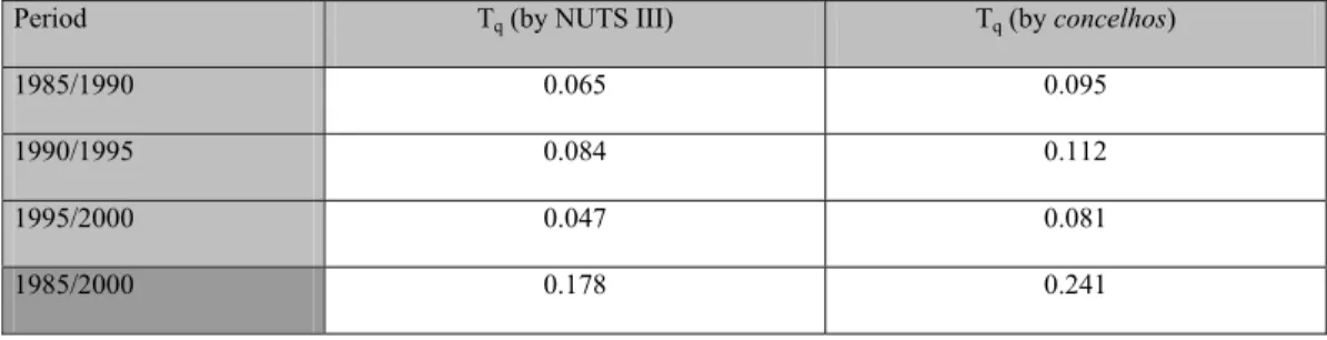
Figure 2 presents the results concerning manufacturing industry as a whole

(Tq), between 1985 and 2000.

[Insert Figure 2 here]

The evidence presented in Figure 2 suggests a significant transformation in the

spatial distribution of manufacturing industry by the Portuguese NUTS III (Tq =

0.178), more remarkable in the sub-period 1990-1995. Calculating the annual

variations in the whole period analyzed, we observe that the spatial transformation is

more evident in the post-Single Market period, namely, by decreasing order, between

1995-1996, 1996-1997 and 1993-1994. These results are strongly corroborated by the

analysis performed at the concelhos level.

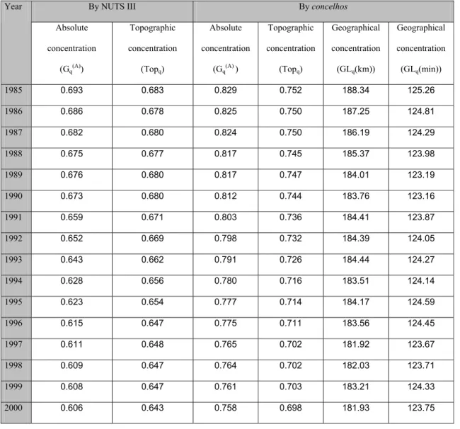
Further evidence on the evolution of spatial concentration of manufacturing

industry is obtained with the indices presented in section 4. Figure 3 shows the results.

Note that in the case of the evaluation by NUTS III, we only use the absolute and the

topographic indices as the geographical index requires information at the concelhos

level and the relative index is adequate only for individual sectors.

[Insert Figure 3 here]

The analysis by NUTS III shows an evident decrease of the absolute and

and TOPq. In fact, according to the two indices considered, the maximum value is

registered in 1985 and the minimum in 2000.

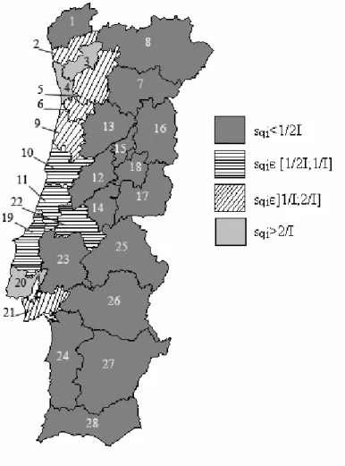
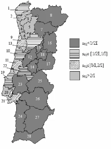
Figures 4 and 5 present a picture of the regional distribution of manufacturing

industry at the NUTS III level in 1985 and 2000, respectively. We have considered

four ranges for the share of manufacturing industry located in each region (sqi).

During the period analyzed, it is possible to observe that manufacturing industry is

mainly concentrated in two major industrial regions: Grande Lisboa in the south

(which includes the political centre of the country and is among the major financial

and economic centres of the Iberian Peninsula) and another one in the north,

consisting on Grande Porto in 1985 and Grande Porto, Ave, Tâmega and Entre

Douro e Vouga in 2000.

[Insert Figures 4 and 5 here]

It is noteworthy that the two regions with the highest share of manufacturing

industry at the beginning of the period analyzed – Grande Lisboa (with 25.8%) and

Grande Porto (with 19.4%) – register a very significant reduction of their share, more

accentuated in the case of Grande Lisboa, which shows the highest reduction among

all regions considered. Serra da Estrela, Península de Setúbal, Algarve and Cova da

Beira also have a reduction in the share of manufacturing industry located in those

regions. Besides, Tâmega, Baixo Vouga and Cávado, all of them with a low share of

manufacturing industry in the beginning of the period, display the most relevant

increases of their shares. This general tendency is confirmed by the correlation

coefficient between sqi1985 and (sqi2000 – sqi1985), as the value obtained (- 0.752) reflects

Turning now our attention to the spatial disaggregation by concelhos, the results

(presented in Figure 3) are concordant with the results for the NUTS III level. In fact,

there is a significant reduction of the degree of absolute and topographic

concentration of manufacturing industry.

In its turn, the geographical concentration index reveals a decrease of the

geographical separation between the regions where manufacturing activity is located

(for instance, GL (min) decreases from 125.26 in 1985 to 123.75 in 2000). Note

however that a decreasing tendency is compatible with a more uniform distribution of

manufacturing industry in the national territory – in line with the picture given by the

remaining indices –, but it can also express a stronger concentration in close regions.

The share of each region in the spatial distribution of manufacturing industry at

the concelhos levelshows that in 1985, the group of three concelhos with the highest

proportion of manufacturing industry comprises Lisboa (17.2%), Porto (5.6%) and

Guimarães (5.2%). At the end of the period, Guimarães, with a value similar to the

one in 1985 (5.3%), comes first in this hierarchy, reflecting a strong reduction of the

relative weight of Lisboa – which had only 3.9% of manufacturing industry in 2000 –

and of Porto – with a share of 2.3% in 2000. The correlation coefficient between

sqi1985 and (sqi2000 – sqi1985) at this spatial disaggregation level (- 0.814) confirms the

result previously presented.

The global conclusion which emerges from the evidence above is that during

the trade liberalization process that followed adhesion to the EU, there was a clear

dispersion of manufacturing industry in the internal Portuguese space. Besides, the

initially more congested areas lost a significant share of manufacturing industry.16

After Portuguese accession to the EU, the specialization pattern of the Portuguese

economy underwent major changes. In parallel with a reduction in the share of the

manufacturing industry, the relative importance of its sub-sectors also changed. The

share of the so-called traditional sectors (wood, cork, paper, skins, leather, textiles,

clothing, footwear) – i.e. those more labor intensive and related to the exploitation of

natural resources – decreased17, while the share of machinery, vehicles and other

transport equipment – the sectors with the highest FDI inflows in terms of foreign

equity in Portuguese manufacturing – increased. In the period 2000-2003, the share of

this last group overcame the traditional one, a notable feature considering the

predominance of the traditional sectors in the past. Despite these changes, in the

2000-2003 period the share of the traditional sectors in total exports was still much

higher for Portugal than was the case for the EU15 average (respectively 33.3% and

8.7%), or even in countries like Spain or Greece.

A global view of the location of individual sectors in the Portuguese case shows

that, in general, traditional sectors that are more intensive in low-skilled labor

predominate in the North (Grande Porto and neighboring regions), while the more

modern sectors (chemicals, metallurgy, machinery and transport) are mainly

concentrated in the Grande Lisboa with a secondary focus in the North (Flôres et al.

2007).

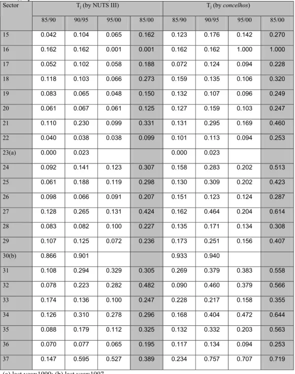
Focusing now our attention on the evolution of the location of each individual

sector at both levels of disaggregation considered in this study, we start, once more,

by evaluating the transformation of the spatial distribution with the Lawrence index

(Tj). Figure 6 presents the results.

[Insert Figure 6 here]

Figure 6 shows a significant transformation of the pattern of sectoral location

mainly in sectors 27 (basic metals) and 32 (radio, television and communication

equipment). Sectors 17 (textiles) and 18 (clothing) – which are predominant in the

Portuguese economy – present intermediate levels of spatial transformation, showing,

respectively, the 6th and 12th position in terms of spatial stability. In an evaluation by

sub-periods, 14 sectors have their highest spatial transformation between 1990 and

1995.

Results at the concelhos level are similar to those for the NUTS III with regard to

the sectors with the sharpest spatial transformation during the period studied.

However, in this case, it is also important to mention sector 34 (motor vehicles),

besides two sectors (16 – tobacco – and 37 – recycling) that are not relevant in the

Portuguese case.

A relevant observation emerging from the results for the Lawrence index in

annual terms, at both levels of disaggregation, is that, confirming the results at the

aggregate level, spatial transformation is more accentuated in the post-Single Market,

suggesting that the above-mentioned studies for the EU space that do not include this

period may have underestimated the real impact of trade openness.

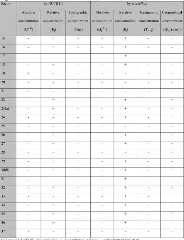
In relation to the evolution of the spatial concentration level of each sector, we

apply the four concepts of concentration considered in section 4. In order to reduce

the vast volume of information that is obtained with calculations at the sectoral level,

Figure 7 indicates whether the sector registers a concentration increase (+) or a

[Insert Figure 7 here]

In what concerns the geographical concentration index, the time evolution of this

index cannot be unequivocally compared with the time evolution of the remaining

concentration indices. For instance, a decrease of this index (which occurs in nine

sectors) shows a reduction of the average distance between the regions where the

sector is located, but this evolution can occur both with a more uniform spatial

distribution of that sector or with a stronger concentration in close regions.

Interestingly enough, a comparison of the time evolution of the three other

concentration indices shows an obvious divergence between the conclusions derived,

on the one hand, from the relative concentration index and, on the other hand, from

the absolute and topographic concentration indices.

Let us observe that in the analysis by NUTS III, 13 sectors reveal an increase of

relative concentration while only 10 sectors show an opposite tendency. In turn, the

analysis based on the absolute index tells us that only sector 19 (leather products and

footwear) registered an increase of concentration during the period studied. The

topographic concentration index corroborates this latter tendency as, according to this

index, only sectors 29 (machinery and equipment n.e.c.) and 30 (office machinery and

computers) became more spatially concentrated.

This dichotomy of results is even more evident when we consider a

disaggregation by concelhos. In fact, the absolute and topographic indices indicate

that no sector increased its spatial concentration, whereas the relative index signals an

increasing tendency in 17 cases.18

How do we explain the distinct message given by the different indices? The main

presupposes the stability of the manufacturing industry at the aggregate level (when

this is the sector taken as reference, as it is usually the case). Nevertheless, in the

present study, we have shown evidence of a strong transformation of the spatial

distribution of the manufacturing industry. This fact causes an increase of the value of

the relative index for each individual sector which is not related to a spatial

transformation of that sector. Therefore, when this is the case, it seems more

appropriate to base the analysis for individual sectors on the absolute and topographic

indices. Our results put a grain of doubt on previous studies that used relative indices

whenever the spatial distribution of manufacturing industry as a whole is not stable in

the period analyzed.

Finally, we evaluate the evolution of the similarity degree of the sectoral

structures of the different regions. An increase of regional specialization will be

expressed in a growing divergence between their sectoral structures. For this purpose,

we calculate the Krugman index in bilateral terms between all the pairs of regions for

each year. With the matrices containing this information, it is possible to obtain, for

each level of disaggregation and for each region, the simple averages in each year,

which give us an indication of the degree of similarity between the sectoral structure

of each region vis-à-vis all the others.

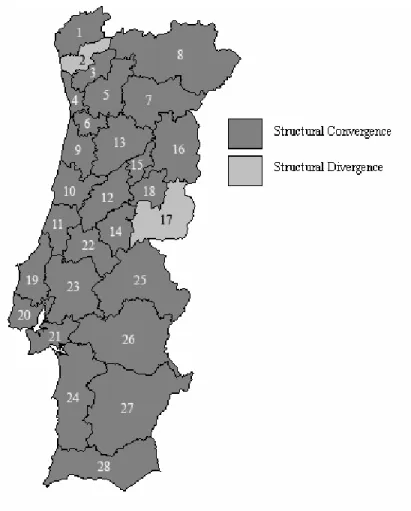
Figure 8 shows, at the NUTS III level, the evolution between 1985 and 2000 of

the degree of similarity between each region and the remaining ones, calculated as

explained above.

Noting that a negative variation signals a convergence of the sectoral structure of

that region with the others while a positive variation means a movement of structural

divergence, Figure 8 clearly suggests that, in the period analyzed, sectoral structures

of the different regions became more similar. In fact, only two NUTS III (Cávado and

Beira Interior Sul) display structural divergence between 1985 and 2000, evaluated in

average bilateral terms. This conclusion is also valid at the concelhos level, as only 66

of them diverged, in average terms, from the others. These results are in line with the

conclusion that emerges from the indices of absolute and topographic concentration

presented above.

6. A relationship between trade and the relocation of manufacturing industry in

Portugal?

The empirical evaluation conducted in the previous section permitted us to

conclude that the period immediately following Portugal’s entry into the EU was

characterized, both at the manufacturing industry level in aggregated terms and in the

majority of sectors considered individually, by a trend to spatial dispersion.

The reduction of the international trading costs is a possible explanation for

the revealed trend. As expressed in the Introduction, entry into the EU brought a

substantial opening up of trade to Portugal. As a result of this opening up to the

exterior, not only the weight of exports in the GDP increased strongly in the period

immediately after EU entry, but Portuguese foreign trade registered an important and

significant change in its geographical direction, in favor of the EU partner countries

2000). However, other factors may also have impacted on the spatial adjustments

observed.

Ideally, the effect of trade openness on the regional disparities should be

evaluated with a formal model. Data constraints related to the number of observations

(16 years) and to the building of some of the explanatory variables hinder such an

attempt.19 However, a discussion of the possible explanatory factors of the spatial

relocation of manufacturing industry in the Portuguese case allows to draw relevant

insights on this topic.

In addition to cross-border trade liberalization, the influence of at least four other

determinants of the relocation of manufacturing industry are worthy of consideration

in the Portuguese case: (i) a structural transformation, with the substitution, in the

most developed and initially most congested regions, of industrial sectors by services

sectors; (ii) the entry of FDI; (iii) the reduction of internal trading costs; and (iv) the

existence of regional policies that favor locations in less congested and less developed

areas, aiming for greater internal cohesion. We continue next with an analysis of the

relevance of each of these four factors during the period under consideration in the

present study.

With regard to structural transformation, identified by Kuznets as one of the main

characteristics of the development process, it is well known that as the regions

develop, they substitute agricultural activities by industrial activities and, at a more

advanced stage, by services.

In Portugal’s case, we can observe that the regions that displayed the highest

levels of concentration in terms of industrial activity in the first year analyzed were

those that registered a greater degree of development. They are situated along the

predominate. Thus, it is possible to believe that between 1985 and 2000, these regions

experienced a substitution of industrial sectors by services, while the regions that

were initially less developed registered a transformation from agricultural to industrial

sectors.

A way to evaluate the validity of this hypothesis consists of complementing the

analysis of the industrial sectors conducted in the preceding sections with a similar

procedure with regard to services.20 Carrying out this analysis enables us to identify

that the dispersion trend found in the industrial sectors is replicated in the service

sectors, as illustrated by three facts. First, the Herfindahl spatial concentration index

was higher for services than for manufacturing industry, but decreasing in both

cases.21 Second, the correlation coefficient between the variation of the share of

manufacturing industry located in each region and the analogous variation for the

service sector in the period analyzed was positive (0.67), pointing to a similar spatial

location trend in both cases. Third, it is of interest to note that the most congested

regions at the beginning of the period (Lisboa and Porto) lost not only manufacturing,

but also services to other regions. Thus, the evidence in relation to the service sectors

does not seem overall to lend support to the hypothesis of structural transformation as

a relevant explanation for the movement observed at the industrial level.

A second explanation for the evidence obtained in the preceding section might be

found in the inward FDI. The flows of FDI into Portugal have been an important

factor in the national economy since joining the EU, with two periods of particularly

strong growth registered during the post-1986 years. The first occurred immediately

after entry, while the second period, which was stronger, took place in the second half

of the 1990s, the effects of which were felt in years later than those analyzed in the

inward FDI contributed to a change in the location profile of manufacturing industry

in Portugal. Indeed, if the multinational companies displayed evidence of a spatially

more dispersed pattern of location, this would help to explain the evidence found.

However, observation of the spatial distribution of the FDI does not corroborate

this hypothesis. Effectively, a highly significant proportion of the FDI flowing into

Portugal in the manufacturing sector is located in the regions that were identified as

having the highest proportion of economic activity.

To illustrate this fact, we turn once again to the information available in the

Ministry of Employment’s Quadros de Pessoal, but this time in relation to

multinational companies. From this information, we verify a high correlation

(approximately 0.70) between the locational distribution (by concelhos) of the total

economic activity and that proportion that refers only to multinational companies

operating in Portugal. Furthermore, and using data for the last year of the period under

analysis, it is possible to verify that the 15 concelhos with the largest volume of

employment in multinational enterprises are all situated in the above-mentioned

coastal strip, in which the greatest proportion of economic activity in global terms is

also concentrated.

A third reason that could be put forward to explain the trend towards industrial

dispersion resides in the reduction of internal trading costs, even if the relation

between reduced transportation costs and the location of economic activity is complex

and non-linear (Krugman, 1991), precluding a clear forecast of the impact of such a

reduction on the location of economic activity.

In fact, from the start of Portugal’s EU membership to the present day, there is

clear evidence of a significant reduction of transportation times and, consequently, of

consequent reductions in journey times and transport costs apparently cannot be put

forward as principal explanations for the trend revealed since, on one hand, the

completion of these projects largely took place after the phase of major structural

transformation of the location profile of Portuguese industry, i.e., the first half of the

1990s (see Table 2), and, on the other hand, the road network built in the first half of

the 1990s, particularly the highways, are strongly concentrated in the regions with the

most significant proportion of the country’s industrial activity.22 This last point is

reinforced if we consider the railway network, which is also concentrated in the

economically most congested areas and where the highest speeds and by far the

greatest volumes of traffic are attained.

Another important reason that could justify the movement from the more central

regions towards the less developed regions may be the existence of regional policies,

conceived at local or national level and designed to attract economic activity to the

less developed regions in order to promote their economic development.

As emphasized by Syrett (1995) and Freitas et al. (2005), in Portugal, the

regional authorities’ policy discretion is very limited. However, some national public

expenditures are closely tied to EU Structural Funds, including the European Regional

Development Fund to reduce regional imbalances, which amounted to roughly 3% of

GDP per year. Portugal also benefited from the Community’s Cohesion Funds that

were introduced in the early 1990s. Together, these funds aimed to promote basic

infrastructures in transport, communication, social infrastructures, incentives to the

business sector and to cross-border cooperation, among other factors that may have

facilitated the spreading out of the firms.

Despite the quantitative importance of these national forms of support, they

Freitas et al. (2005) have shown, for the period 1995-2000, a divergence between the

Portuguese regions both in per-capita and gross value added per-worker terms. One of

the factors contributing to this divergence could have been the fact that in certain

periods, in particular during the time that the Second Community Support Framework

was in force, the funding per capita for the poorest regions was substantially lower

than that for the richest regions (Freitas et al., 2005).

In conclusion, all of these potentially explanatory factors do not seem to

explain sufficiently the evidence presented in the preceding section, leaving the

reduction of international trading costs as a reasonable explanation for the trend

observed.

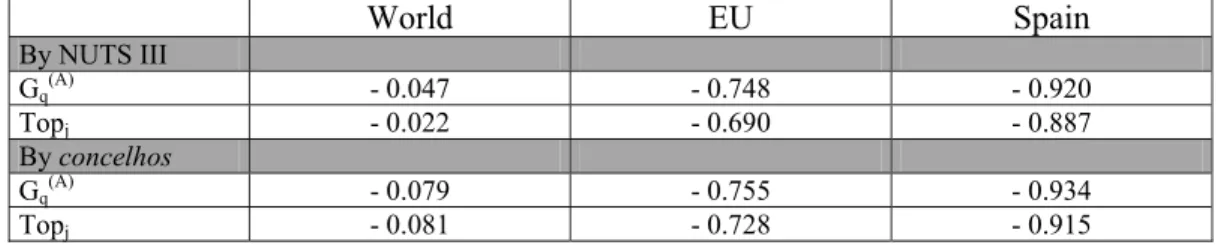
A simple way of evaluating the relation between trade liberalization and the

industrial dispersion trend revealed in Portugal is to calculate the correlation

coefficient between the measurements of spatial concentration used in the preceding

section and a measurement of trade intensity.23 The results of this calculation are

presented below in Figure 9, which considers this relation for the world, the EU space

and the case of Spain.

Among EU partners, the importance of Spain must indeed be stressed. In spite of

being the only country with which Portugal shares a common frontier, trade between

both countries remained at low levels before 1986. In part the reason is related to the

fact that, in spite of a resurgence of import substitution during the latter-1970s and

early 1980s, basically made up of non-tariff barriers (Fontoura and Valério, 1994),

Portuguese trade on industrial goods became progressively free of tariffs since the

beginning of the 1970s with EU members. In contrast, high levels of commercial

protectionism were maintained with Spain until both countries joined the EU. As

industrial goods), the weight of this country in Portugal’s trade increased substantially

(Portuguese exports to this country increased from 4.1% to 19.3% between 1985 and

2000, while imports from Spain into Portugal rose from 7.4% to 25.9% in the same

period). In the end of the period analyzed, Spain was already the principal trading

partner of Portugal.

[Insert Figure 9 here]

The results presented in Figure 9 suggest that the increased importance of

trade in the Portuguese case is clearly (and negatively) associated with the level of

spatial concentration of industry in the Portuguese internal space, both when the

evaluation is based on a spatial disaggregation by NUTS III and by concelhos. This

assertion is particularly relevant to the EU case, but even more so in relation to Spain.

In both cases, trade liberalization and the subsequent reduced costs of international

trade have more significance in the post-EU entry phase.

Interestingly enough is the fact that the calculations made in Section 5, above

all at the level of concelhos, show that the regions with the highest proportion of

manufacturing industry and in which the most significant reduction of industrial

presence took place are those which are most distant from the Spanish frontier.

Therefore, the reduction of international trading costs appears to have led, taking into

account the importance of the trading relations with Spain, to industrial dispersion to

regions that are less congested and nearer to the frontier with Spain.

To sum up, the evidence presented in this section seems to indicate that the

reduction of international trading costs has contributed significantly to explaining the

7. Final remarks

The empirical analysis for Portugal between 1985 and 2000 concerning

manufacturing industry shows a dispersion of this economic activity, both at the

aggregate level and for individual sectors.

The evidence for the aggregated manufacturing industry is in line with the

hypothesis established by KE. In fact, it is our contention that while several factors

may have contributed to determine the industrial spatial adjustments observed in this

study, trade openness was relevant and, apparently, the most important.

At first glance the dispersion movement observed is contradictory to the fact that,

in the Portuguese case, labor mobility is restricted, since there is a high level of job

protection and high private costs to geographic mobility due to housing market

restrictions. Apparently, congestion costs in the more concentrated regions were the

prevalent centrifugal force that led to spatial decisions.

On the other hand, we conclude that individual sectors became more dispersed

in the Portuguese territory in the period analyzed, leading to convergence between the

different regions in terms of their sectoral structure. This result is in contrast to what

has been predicted by Fujita et al. (1999), pointing to the need for future research on

the spatial adjustments of individual sectors, both in theoretical and empirical terms. It

is possible that the decisive determinants of within-sectors’ locational decisions are

related to sectoral characteristics, as shown for instance by Faber (2007) for the

Mexican case.

Finally, as mentioned in the Introduction, it has been assumed that structural

convergence should lead to real convergence. However, there is no evidence of real

Other factors may thus have explained the increased regional inequalities in the

standards of living, counteracting the benefits of increased dispersion of

manufacturing industry.

References

ADES, A. and GLAESER, E. (1995) Trade and Circuses: Explaining Urban Giants,

Quarterly Journal of Economics, 110, pp. 195-227.

ALONSO-VILLAR, O. (2001) Large Metropolises in the Third World: An

Explanation, Urban Studies, 38(8), pp. 1359-1371.

ARIAS, A. (2003) Trade Liberalization and Growth: Evidence from Mexican Cities,

The International Trade Journal, 17(3), pp. 253-273.

BALDWIN, R. (1999) Agglomeration and Endogenous Capital, European Economic

Review, 43, pp. 253-280.

BALDWIN, R. and FORSLID, R. (1999) The Core-Periphery Model and Endogenous

Growth, CEPR Discussion Paper No. 1749.

BEHRENS, K. (2003) International Trade and Internal Geography Revisited,

BEHRENS, K., GAIGNÉ, C., OTTAVIANO, G. and THISSE, J. (2003)

Inter-Regional and International Trade: Seventy Years After Ohlin, CEPR Discussion

Paper No. 4065.

BRÜLHART, M. (2001) Evolving Geographical Concentration of European

Manufacturing Industries, Weltwirtschaftliches Archiv,137(2), pp. 215-243.

BRÜLHART, M. and TRAEGER, R. (2005) An Account of Geographic

Concentration Patterns in Europe, Regional Science and Urban Economics, 35(6), pp.

597-624.

CROZET, M. and SOUBEYRAN, P. (2004) EU Enlargement and the Internal

Geography of Countries, Journal of Comparative Economics, 32(2), pp. 265-279.

DE ROBERTIS, G. (2001) European Integration and Internal Economic Geography:

the Case of the Italian Manufacturing Industry 1971-1991, The International Trade

Journal, 15(3), pp. 345-371.

DIXON, R. and THIRLWALL, A. (1975) A Model of Regional Growth-Rate

Differences on Kaldorian Lines, Oxford Economic Papers, 27(2), pp. 201-214.

FABER, B. (2007) Towards the Spatial Patterns of Sectoral Adjustments to Trade

Liberalisation: the Case of NAFTA in Mexico, Growth and Change, 38(4), pp.

FLÔRES, R., FONTOURA, M. and SANTOS, R. (2007) Foreign Direct Investment

and Spillovers: Additional Lessons from a Country Study, The European Journal of

Development Research, 19(3), pp. 372-390

FONTOURA, M. and VALÉRIO, N. (1994) Protection, Foreign Trade and Economic

Growth in Portugal: 1840's-1980's: a Long Term View, in P. Lindert, Nye, J. and

Chevet, J-M. (eds.) Political Economy of Protectionism and Commerce, 18th-20th

centuries. Milan, 11th International Economic History Congress, pp. 77-87.

FREITAS, M., TORRES, F., AMORIM, C., BONGARDT, A., DIAS, M. and

SILVA, R. (2005) Regional Convergence in Portugal: Policy Impacts (1990-2001),

Working Paper E/nº 35, Universidade de Aveiro.

FUJITA, M., KRUGMAN, P. and VENABLES, A. (1999) The Spatial Economy:

Cities, Regions and International Trade, Cambridge: MIT Press.

HANSON, G. (1998) Regional Adjustment to Trade Liberalization, Regional Science

and Urban Economics, 28(4), pp. 419-444.

HENDERSON, J. (1996) Ways to Think About Urban Concentration: Neoclassical

Urban Systems Versus the New Economic Geography, International Regional

Science Review, 19(1 and 2), pp. 31-36.

HIRSCHMAN, A. (1958) Strategy of Economic Development, New Haven: Yale

ISSERMAN, A. (1996) It’s Obvious, It’s Wrong, and Anyway They Said It Years

Ago? Paul Krugman on Large Cities, International Regional Science Review, 19(1

and 2), pp. 37-48.

KEEBLE, D., OFFORD, J. and WALKER, S. (1988) Peripheral Regions in a

Community of Twelve Member States, Report for the European Commission, Brussels.

KRUGMAN, P. (1991) Increasing Returns and Economic Geography, Journal of

Political Economy, 99, pp. 483-499.

KRUGMAN, P. and HANSON, G. (1993) Mexico-U.S. Free Trade and the Location

of Production, in P. Garber (ed.) The Mexico-U.S. Free Trade Agreement, Cambridge:

MIT Press.

KRUGMAN, P. and ELIZONDO, R. (1996) Trade Policy and the Third World

Metropolis, Journal of Development Economics, 49, pp. 137-150.

LAWRENCE, R. (1984) Can America Compete? Washington D.C.: The Brookings

Institution.

LEICHENKO, R. and SILVA, J. (2004) International Trade, Employment, and

MANSORI, K. (2003) The Geographic Effects of Trade Liberalization with

Increasing Returns in Transportation, Journal of Regional Science, 43(2), pp.

249-268.

MARTIN, P. and OTTAVIANO, G. (1999) Growing Locations: Industry Location in

a Model of Endogenous Growth, European Economic Review, 43(2), pp. 281-302.

MARTIN, R and SUNLEY, P. (1996) Paul Krugman’s Geographical Economics and

its Implications for Regional Development Theory: A Critical Assessment, Economic

Geography,72(3), pp. 259-292.

McCANN, P (2005) Transport Costs and New Economic Geography, Journal of

Economic Geography, 5(3), pp. 305-318.

MIDELFART-KNARVIK, K., OVERMAN, H., REDDING, S. and VENABLES, A.

(2000) The Location of European Industry, The European Commission Directorate

General for Economic and Financial Affairs, Economic Papers No. 142.

MIDELFART-KNARVIK, K., OVERMAN, H., REDDING, S. and VENABLES, A.

(2002) Integration and Industrial Specialisation in the European Union, Révue

Économique, 53(3), pp. 469-481.

MONFORT, P. and NICOLINI, R. (2000) Regional Convergence and International

MONFORT, P. and VAN YPERSELE, T. (2003) Integration, Regional

Agglomeration and International Trade, CEPR Discussion Paper No. 3752.

MYRDAL, G. (1957) Economic Theory and Underdeveloped Regions, London:

Duckworth.

NITSCH, V. (2001) Openness and Urban Concentration in Europe, 1870-1990,

HWWA Discussion Paper No. 121.

NITSCH, V. (2003) Trade Openness and Urban Concentration: New Evidence, paper

presented at the European Trade Study Group Conference, Madrid, 11-13 September.

PALUZIE, E. (2001) Trade Policy and Regional Inequalities, Papers in Regional

Science, 80, pp. 67-85.

PALUZIE, E., PONS, J. and TIRADO, D. (2001) Regional Integration and

Specialization Patterns in Spain, Regional Studies, 35(4), pp. 285-296.

PRED, A. (1966) The Spatial Dynamics of US Urban-Industrial Growth, 1800-1914,

Cambridge: MIT Press.

RODRÍGUEZ-POSE, A. and GILL, N. (2006) How Does Trade Affect Regional

RODRÍGUEZ-POSE, A. and SÁNCHEZ-REAZA, J. (2002) Economic Polarisation

through Trade: the Impact of Trade Liberalization on Mexico’s Regional Growth,

paper presented at the Cornell/LSE/Wider Conference on Spatial Inequality and

Development, London School of Economics.

SILVA, J. and LEICHENKO, R. (2004) Regional Income Inequality and International

Trade, Economic Geography, 80(3), 261-286.

SYRETT, S. (1995) Local Development, Hong Kong: Avebury.

STORPER, M., CHEN, y. AND DE PAOLIS, F. (2002) Trade and the Location of

Industries in the OECD and European Union, Journal of Economic Geography, 2(1),

Figure 1 - Concepts of spatial concentration

Concentration concept

Index Question to evaluate Maximum concentration Minimum concentration

Absolute Gj (A)

Is sector j concentrated in

many or few regions?

Sector j is in only one

region

Sector j is evenly

distributed by all regions

Relative Ej How similar are the

spatial distributions of

sector j and of the total

economic activity?

Maximum divergence

between the distributions

of sector j and that of the

total economic activity

(where sector j is located,

there are no other sectors)

The distribution of sector

j is identical to that of

total economic activity

Topographic TOPj Is sector j uniformly

distributed in the space?

Sector j is fully

concentrated in the

smallest region

Sector j has a spatial

uniform distribution

Geographical GLj Is sector j located in close

or distant regions?

Sector j is fully

concentrated in the

smallest region (a)

Sector j is equally

distributed by the two

regions which are the

most distant from each

other (b)

Figure 2 - Structural transformation of the spatial distribution of manufacturing industry, 1985-2000

Period Tq (by NUTS III) Tq (by concelhos)

1985/1990 0.065 0.095

1990/1995 0.084 0.112

1995/2000 0.047 0.081

Figure 3 - Level of spatial concentration of manufacturing industry by NUTS III and

concelhos, 1985-2000

By NUTS III By concelhos

Year

Absolute

concentration

(Gq(A))

Topographic

concentration

(Topq)

Absolute

concentration

(Gq(A) )

Topographic

concentration

(Topq)

Geographical

concentration

(GLq(km))

Geographical

concentration

(GLq(min))

1985 0.693 0.683 0.829 0.752 188.34 125.26

1986 0.686 0.678 0.825 0.750 187.25 124.81

1987 0.682 0.680 0.824 0.750 186.19 124.29

1988 0.675 0.677 0.817 0.745 185.37 123.98

1989 0.676 0.680 0.817 0.747 184.01 123.19

1990 0.673 0.680 0.812 0.744 183.76 123.16

1991 0.659 0.671 0.803 0.736 184.41 123.87

1992 0.652 0.669 0.798 0.732 184.39 124.05

1993 0.643 0.662 0.791 0.726 184.44 124.27

1994 0.628 0.656 0.780 0.716 183.51 124.14

1995 0.623 0.654 0.777 0.714 184.17 124.59

1996 0.615 0.647 0.775 0.711 183.56 124.45

1997 0.611 0.648 0.765 0.702 181.92 123.67

1998 0.609 0.647 0.764 0.702 182.03 123.71

1999 0.608 0.647 0.761 0.703 183.21 124.33

Figure 4 - Spatial distribution of manufacturing industry by NUTS III (1985)

1-Minho-Lima; 2-Cávado; 3-Ave; 4-Grande Porto; 5-Tâmega; 6-Entre Douro e Vouga; 7-Douro; 8-Alto Trás-os-Montes; 9-Baixo Vouga; 10-Baixo Mondego; 11-Pinhal Litoral; 12-Pinhal Interior Norte; 13-Pinhal Interior Sul; 14-Dão-Lafões; 15 - Serra da Estrela; 16-Beira Interior Norte; 17-Beira Interior Sul; 18-Cova da Beira; 19-Oeste; 20-Grande Lisboa; 21-Península de Setúbal; 22-Médio Tejo; 23-Lezíria do Tejo; 24-Alentejo Litoral; 25-Alto Alentejo; 26-Alentejo Central; 27-Baixo Alentejo; 28-Algarve.

Figure 5 - Spatial distribution of manufacturing industry by NUTS III (2000)

Figure 6 - Transformation of the spatial distribution of the manufacturing sectors (2 digit level), by NUTS III and concelhos, 1985-2000

Tj (by NUTS III) Tj (by concelhos)

Sector

85/90 90/95 95/00 85/00 85/90 90/95 95/00 85/00

15 0.042 0.104 0.065 0.162 0.123 0.176 0.142 0.270

16 0.162 0.162 0.001 0.001 0.162 0.162 1.000 1.000

17 0.052 0.102 0.058 0.188 0.072 0.124 0.094 0.228

18 0.118 0.103 0.066 0.273 0.159 0.135 0.106 0.320

19 0.083 0.065 0.048 0.150 0.132 0.107 0.096 0.249

20 0.061 0.067 0.061 0.125 0.127 0.159 0.103 0.247

21 0.110 0.230 0.099 0.331 0.131 0.295 0.169 0.460

22 0.040 0.038 0.038 0.099 0.101 0.113 0.094 0.253

23(a) 0.000 0.023 0.000 0.023

24 0.092 0.141 0.123 0.307 0.158 0.283 0.202 0.513

25 0.061 0.188 0.119 0.298 0.130 0.309 0.202 0.423

26 0.098 0.066 0.091 0.207 0.151 0.123 0.124 0.287

27 0.128 0.265 0.131 0.424 0.162 0.464 0.204 0.614

28 0.083 0.082 0.100 0.227 0.135 0.171 0.134 0.308

29 0.107 0.125 0.072 0.236 0.173 0.251 0.156 0.407

30(b) 0.866 0.901 0.933 0.940

31 0.108 0.294 0.329 0.305 0.269 0.379 0.383 0.558

32 0.078 0.223 0.282 0.482 0.090 0.460 0.379 0.566

33 0.174 0.136 0.100 0.247 0.228 0.217 0.158 0.355

34 0.126 0.310 0.278 0.296 0.168 0.404 0.472 0.644

35 0.088 0.179 0.112 0.325 0.132 0.332 0.203 0.563

36 0.070 0.077 0.065 0.195 0.117 0.134 0.094 0.253

37 0.147 0.595 0.527 0.389 0.234 0.757 0.707 0.719

Figure 7 - Evolution of the levels of concentration by NUTS III and concelhos, 1985-2000

by NUTS III by concelhos

Sector

Absolute

concentration

(Gj(A))

Relative

concentration

(Ej)

Topographic

concentration

(Topj)

Absolute

concentration

(Gj(A) )

Relative

concentration

(Ej)

Topographic

concentration

(Topj)

Geographical

concentration

(GLj (min))

15 - + - - + - +

16 - + - - + - -

17 - - - - + - -

18 - + - - + - -

19 + - - - - - -

20 - - - - - - -

21 - - - - - - +

22 - + - - + - +

23(a) = + = = + = =

24 - - - - + - +

25 - - - - - - -

26 - + - - + - +

27 - + - - + - +

28 - - - - - - +

29 - + + - + - -

30(b) - + + - + - +

31 - - - - + - -

32 - + - - + - +

33 - - - - + - +

34 - + - - + - +

35 - + - - + - +

36 - + - - + - -

37 - - - - - - +