Geometric Semantic Inspired Mutation for M3GP
Ana Sofia Brás Pinto
Dissertation presented as partial requirement for obtaining
the Master’s degree in Advanced Analytics
Universidade NOVA de Lisboa
NOVA Information Management School
Geometric Semantic Inspired Mutation for
M3GP
Ana Sofia Br´
as Pinto
Supervisor: Doctor Leonardo Vanneschi
Dissertation presented as a partial requirement for obtaining the Master's degree in Advanced Analytics
Abstract
One of the most challenging Machine Learning tasks is multiclass classification. Genetic Programming (GP) is not able to achieve a very good performance when applied to classifica-tion problems with number of classes bigger than two. However, Multidimensional Multiclass Genetic Programming (M2GP) and Multidimensional Multiclass Genetic Programming with Multidimensional Populations (M3GP), two wrapper-based GP classifiers, have shown to be competitive with state-of-the-art classifiers.
The main focus of this work is a new version of M3GP, called Geometric Semantic In-spired M3GP (GSI-M3GP), inIn-spired in geometric semantic operators. GSI-M3GP works in the same way as M3GP, but uses only three operators to create new individuals: add branch, remove branch and a new mutation operator called geometric semantic inspired mutation (gsi-mutation).
In order to test GSI-M3GP and compare it to M3GP, an implementation in Java was de-veloped. Nine different versions of GSI-M3GP were created and tested on eight benchmark problems. For most of the versions of GSI-M3GP, the new algorithm is competitive with M3GP on all the problems. Additionally, it was tested if adding a crossover operator would improve the results, which it did not. A few other alterations were made to the original M3GP algorithm to test the possibility of using the Euclidean distance, instead of the Mahalanobis distance, without harming the quality of the solutions. These alterations do not always main-tain the quality of the solutions.
Keywords: Machine Learning, Multiclass Classification, Genetic Programming, Geometric Semantic Genetic Programming,...
Resumo
Uma das tarefas mais desafiantes de Aprendizagem Autom´atica ´e classifica¸c˜ao em mais de duas classes. Genetic Programming (GP) n˜ao consegue obter um bom desempenho nestes problemas. No entanto, Multidimensional Multiclass Genetic Programming (M2GP) e Multi-dimensional Multiclass Genetic Programming with MultiMulti-dimensional Populations (M3GP), dois algoritmos de classifica¸c˜ao que utilizam GP como m´etodo wrapper, mostraram ser competitivos com classificadores do estado-de-arte.
O foco deste trabalho ´e a cria¸c˜ao de uma nova vers˜ao de M3GP, chamada Geometric Semantic Inspired M3GP (GSI-M3GP), inspirada em operadores da geometria semˆantica. GSI-M3GP funciona da mesma forma que M3GP, mas utiliza apenas trˆes operadores para criar novos indiv´ıdulos: adicionar dimens˜ao, remover dimens˜ao e um novo operador de muta¸c˜ao, de nome geometric semantic inspired mutation (gsi-mutation).
Para testar GSI-M3GP e compar´a-lo com M3GP, foi criada uma implementa¸c˜ao em Java. Foram testadas nove vers˜oes diferentes de M3GP em oito problemas de benchmark. GSI-M3GP ´e competitivo com M3GP em todos os problemas considerados. Foi ainda testado se adicionar um operador de crossover melhoraria os resultados, mas tal n˜ao se verificou. Outras altera¸c˜oes foram feitas a M3GP de forma a testar a possibilidade de utilizar a distˆancia Eu-clideana em vez da distˆancia de Mahalanobis, sem que a qualidade das solu¸c˜oes fosse afetada. Estas altera¸c˜oes nem sempre mantˆem a qualidade das solu¸c˜oes.
Palavras-chave: Aprendizagem Autom´atica, Classifica¸c˜ao em mais de duas classes, Genetic Programming, Geometric Semantic Genetic Programming,...
Acknowledgements
I would like to express my gratitude towards my supervisor, professor Leonardo Vanneschi. For the enthusiasm he shows while teaching and the way he passes his enthusiasm to the students. For his availability and for giving me the opportunity to work on the amazing idea he had and the operator he created. I would also like to thank professor Sara Silva and her student, Jo˜ao Batista, for helping me with some details of M3GP while I was implementing my own code. I would like to thank professor Jorge Mendes for providing useful book references in statistics.
I would also like to thank Susana and Carina, the amazing women with whom I shared my path during the masters of Advanced Analytics. Susana, without you the first year would not have been the same. I learned so much from you, you are a true inspiration and friend. Carina, thank you for your support during this second year, you made it much easier and fun to handle. Thank you for believing in me the same way I believe in you.
Finally, I would like to express how grateful I am for the people that have always been and will always be here for me: my family and friends. Special acknowledgements go to my two favourite physicists, my brother, my dad and my mum. Thank you to Bruno for being the friend everyone would love to have. No words that can express how much I am thankful for you Pepas - thank you for always being my home. Thank you to my brother, for the eternal love and caring. Obrigada m˜ae e pai, por fazerem tudo ao vosso alcance por mim.
‘The important thing is not to stop questioning. Curiosity has its own reason for existing.’ Albert Einstein
Contents
1 Introduction 1 2 Background Theory 3 2.1 Machine Learning . . . 3 2.1.1 Supervised Learning . . . 4 2.2 Evolutionary Algorithms . . . 4 2.2.1 Genetic Programming . . . 52.2.2 Geometric Semantic Genetic Programming (GSGP) . . . 11
2.3 Multiclass classification problems and algorithms . . . 14
2.3.1 Multidimensional multiclass Genetic Programming (M2GP) . . . 15
2.3.2 M2GP with Multidimensional Populations (M3GP) . . . 22
3 M3GP algorithm original results 25 3.1 Experimental setup and results . . . 25
3.1.1 Original results . . . 27
3.1.2 M3GP with a smaller population . . . 28 v
vi CONTENTS
4 General changes to M3GP 30
4.1 M3GP-N: Min-Max Normalization . . . 31
4.2 M3GP-S: Standardization . . . 33
4.3 Results and comparison to original M3GP . . . 34
5 Geometric semantic inspired mutation for M3GP 41 5.1 The new mutation operator . . . 42
5.2 GSI-M3GP variants: how to choose the moving point ? . . . 52
5.2.1 Baseline . . . 53 5.2.2 Hyperrectangle . . . 53 5.2.3 Hyperellipse . . . 54 5.2.4 Donut . . . 60 5.2.5 Misclassified . . . 61 5.2.6 Misclassified-hyperrectangle . . . 61 5.2.7 Misclassified-hyperellipse . . . 61 5.2.8 Around Misclassified . . . 62 5.2.9 Correct-Misclassified distances . . . 63
5.3 Experimental Setup and Results . . . 71
5.3.1 Baseline . . . 72
5.3.2 Hyperrectangle . . . 80
5.3.3 Hyperellipse . . . 102
5.3.4 Donut . . . 117
5.3.6 Misclassified-hyperrectangle . . . 120
5.3.7 Misclassified-hyperellipse . . . 123
5.3.8 Around Misclassified . . . 125
5.3.9 Correct-Misclassified distances . . . 132
6 GSI-M3GP-XO: adding crossover 140 6.1 Experimental Setup and Results . . . 141
7 Implementation issues of M3GP 148 7.1 Training set and test set . . . 148
7.2 Covariance matrices . . . 149
7.2.1 What if a covariance matrix is not invertible? . . . 149
7.2.2 What matrices are considered to be invertible? . . . 149
7.3 Dimensions of a tree . . . 152 8 Conclusions 154 8.1 Summary of Contributions . . . 154 8.2 Future Work . . . 155 Bibliography 155 vii
List of Tables
3.1 Description of the datasets used for the experimental analysis. . . 25 3.2 Running parameters of M3GP. . . 26 3.3 Comparison between the original[15, 17] and new implementation of M3GP. . . 27 3.4 Comparison between M3GP with 500 individuals and 50 individuals. . . 28
4.1 Comparison between the M3GP, M3GP-N and M3GP-S. . . 34
5.1 Comparison between the number of nodes of a 1-dimensional individual to which the mutation operator has been applied n times using betw(yi, ci) and betw(fi(x), ci) (considering individuals created with 6-depth full method [11]). . . 51 5.2 Probability of finding a point inside the hyperellipse, given that the point was
generated inside the hyperrectangle, according to the number of dimensions, d. The values of ai represent the sizes of the hyperellipses axes’ half-lengths. . . 57
5.3 Number of points to generate given the number of dimensions,d, of the individual. 58 5.4 Comparison between distances to centroid according to the operator,
classifica-tion and particlassifica-tion, where avg referes to average and med refers to median. . . . 64 5.5 Relative change on: (Train) the average distances for the correctly classified
mapped training samples and the misclassified mapped training samples; (Test) the average distances for the correctly classified mapped test samples and the misclassified mapped test samples; (Misc) the average distances for the misclas-sified mapped training samples and the misclasmisclas-sified mapped test samples. . . . 66
x LIST OF TABLES
5.6 Percentage of individuals for whom there was an increasing between . . . 67 5.7 Running parameters of GSI-M3GP. . . 71 5.8 Comparison between the M3GP and GSI-M3GP Baseline 0.0001%, Baseline 1%
and Baseline 10% variants. . . 73 5.9 Comparison between Baseline 0.0001%, Baseline 1% and Baseline 10% depth
values. . . 74 5.10 Comparison between Baseline 0.0001%, Baseline 10% and Baseline 1% operators’
percentages . . . 74 5.11 Comparison between Baseline 0.0001%, Baseline 10% and Baseline 1% number
of operations. . . 75 5.12 Comparison between the M3GP and GSI-M3GP hyperrectangle variants with
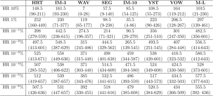
pred% equal to 10k%, with k ∈ {1, 0, −1, ..., −6}. . . . . 81
5.13 Comparing depth values between GSI-M3GP hyperrectangle variants with pred% equal to 10k%, with k ∈ {1, 0, −1, ..., −6}. . . . . 82
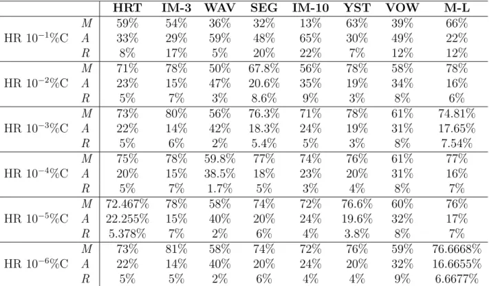
5.14 Comparing operators’ percentages between the GSI-M3GP hyperrectangle vari-ants with pred% equal to 10k%, with k ∈ {1, 0, −1, ..., −6}. . . . 82
5.15 Comparing the number of operations between the GSI-M3GP hyperrectangle variants with pred% equal to 10k%, with k ∈ {1, 0, −1, ..., −6}. . . . . 83
5.16 Comparison between the M3GP and GSI-M3GP hyperrectangle variants with pred% equal to 10k%, with k ∈ {1, 0, −1, ..., −6}, and r
i = 0. . . 84
5.17 Comparing depth values between GSI-M3GP hyperrectangle variants with pred% equal to 10k%, with k ∈ {1, 0, −1, ..., −6}, and r
i = 0. . . 84
5.18 Comparing operators’ percentages between the GSI-M3GP hyperrectangle vari-ants with pred% equal to 10k%, with k ∈ {1, 0, −1, ..., −6}, and r
i = 0. . . 85
5.19 Comparing the number of operations between the GSI-M3GP hyperrectangle variants with pred% equal to 10k%, with k ∈ {1, 0, −1, ..., −6}, and ri = 0. . . . 86
LIST OF TABLES xi
5.20 Comparison between the M3GP and GSI-M3GP hyperrectangle variants with
pred% ∈]0, 10k]%, with k ∈ {−1, −2, −3}. . . . . 93
5.21 Comparing depth values between GSI-M3GP hyperrectangle variants with pred% ∈ ]0, 10k]%, with k ∈ {−1, −2, −3}. . . . 94
5.22 Comparing operators’ percentages between the GSI-M3GP hyperrectangle vari-ants with pred% ∈]0, 10k]%, with k ∈ {−1, −2, −3}. . . . 94
5.23 Comparing the number of operations between the GSI-M3GP hyperrectangle variants with pred% ∈]0, 10k]%, with k ∈ {−1, −2, −3}. . . . 95
5.24 Comparison between M3GP, HE χ2 99%, HE χ 2 50% and HE χ 2 25%. . . 103 5.25 Comparison between HE χ2 99%, HE χ250% and HE χ225% depth values. . . 103
5.26 Comparison between HE χ2 99%, HE χ 2 50% and HE χ 2 25% operators’ percentages. . . 104
5.27 Comparing the number of operations between HE χ2 99%, HE χ250% and HE χ225%. 104 5.28 Comparison between M3GP and HE χ2 99% and χ 2 50%. . . 110
5.29 Comparison between M3GP and HE χ2 99% and χ250% depth values. . . 110
5.30 Comparison between M3GP and HE χ2 99% and χ 2 50% operators’ percentages. . . . 111
5.31 Comparing the number of operations between M3GP and HE χ2 99% and χ250%. . . 111
5.32 Comparison between M3GP and the Donut variant of GSI-M3GP. . . 117
5.33 GSI-M3GP Donut variant depth values. . . 117
5.34 GSI-M3GP Donut variant operators’ percentages. . . 118
5.35 GSI-M3GP Donut variant number of operations. . . 118
5.36 Comparison between M3GP and the Misclassified variant of GSI-M3GP. . . 120
5.37 Comparison between M3GP and the MHR variant of GSI-M3GP. . . 121
5.38 GSI-M3GP MHR variant depth values. . . 121
xii LIST OF TABLES
5.40 GSI-M3GP MHR variant number of operations. . . 122
5.41 Comparison between M3GP, MHE χ299% and MHE χ210%. . . 123
5.42 Comparison between MHE χ299% and MHE χ210% depth values. . . 123
5.43 Comparison between MHE χ2 99% and MHE χ210% operators’ percentages. . . 124
5.44 Comparing the number of operations between MHE χ2 99% and MHE χ 2 10%. . . 124
5.45 Comparison between M3GP, AM0.5σ, AM1σ and AM2σ. . . 126
5.46 Comparison between AM0.5σ, AM1σ and AM2σ depth values. . . 127
5.47 Comparison between AM0.5σ, AM1σ and AM2σ operators’ percentages. . . 127
5.48 Comparing the number of operations between AM0.5σ, AM1σ and AM2σ. . . . 127
5.49 Comparison between M3GP, AM10% and AM25%. . . 130
5.50 Comparison AM10% and AM25% depth values. . . 130
5.51 Comparison AM10% and AM25% operators’ percentages. . . 130
5.52 Comparing the number of operations between AM10% and AM25% depth values. 130 5.53 Comparison between M3GP, CMD AVG-A, CMD AVG-C, CMD MED-A and CMD MED-C. . . 133
5.54 Comparison between CMD AVG-A, CMD AVG-C, CMD MED-A and CMD MED-C depth values. . . 133
5.55 Comparison between CMD AVG-A, CMD AVG-C, CMD MED-A and CMD MED-C operators’ percentages. . . 134
5.56 Comparing the number of operations between CMD AVG-A, CMD AVG-C, CMD MED-A and CMD MED-C. . . 134
5.57 Comparison between M3GP, CMD MED-A 25% and CMD MED-A 100%. . . . 136 5.58 Comparison between CMD MED-A 25% and CMD MED-A 100% depth values. 136
5.59 Comparison between CMD MED-A 25% and CMD MED-A 100% operators’ percentages. . . 137 5.60 Comparing the number of operations between CMD MED-A 25% and CMD
MED-A 100%. . . 137
6.1 Running parameters of GSI-M3GP-XO. . . 141 6.2 Comparison between M3GP, HR, HR-XO EP, HR-XO X&M, AM1σ, AM1σ-XO
EP and AM1σ-XO X&M. . . 142 6.3 Comparison between HR, HR-XO EP, HR-XO X&M, AM1σ, AM1σ-XO EP and
AM1σ-XO X&M depth values. . . 143 6.4 Comparison between HR, HR-XO EP, HR-XO X&, AM1σ, AM1σ-XO EP and
AM1σ-XO X&M operators’ percentages. . . 144 6.5 Comparing the number of operations between HR, HR-XO EP, HR-XO X&M,
AM1σ, AM1σ-XO EP and AM1σ-XO X&M. . . 144
List of Figures
2.1 GP program/individual. . . 6
2.2 Example of a GP individual created using method Full, with maximum depth equal to two. . . 7
2.3 Examples of GP individuals created using method Grow, with maximum depth equal to two. From left to right, the trees have, respectively, depth of 2, 1 and 0. 8
2.4 Example of individuals generated by the crossover operator. . . 10
2.5 Example of an individual generated by the mutation operator. The random tree was generated using grow. . . 11
2.6 Representation of the genotypic space (where individuals are represented by their trees) versus the semantic space (where the individuals are represented by their semantics). The semantic space is 2-dimensional since one is considering a toy example of a dataset with only 2 instances. The star corresponds to the target. . 12
2.7 Toy example of the application of the geometric semantic mutation. T1, T2,...,T6 is a sequence of trees to which the geometric semantic mutation is applied, where Ti+1 is generated by applying the operator to Ti. By generating a tree using the mutation operator, the semantics of the offspring is inside a grey square (since the semantic space is 2-dimensional, because one is considering a dataset with 2 instances) with center in the semantics of the parents. There is always a chance of improvement, as expressed here. The star represents que target. . . 13
xvi LIST OF FIGURES
2.8 Example of applying the geometric semantic crossover operator to two parent trees. The offspring has semantics falling in the line segment joining the seman-tics of the parents, so the offspring might be closer to the target - the offspring is not worse than the worst of the parents. The semantic space is bi-dimensional since a 2 instance dataset is being considered, for simplicity. The star represents the target. . . 13 2.9 Example of a one-dimensional tree and a two-dimensional tree. . . 16
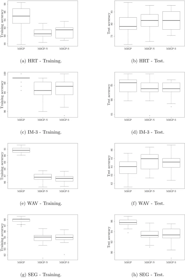
4.1 A possible M3GP solution. . . 31 4.2 Comparison between median accuracies ofM3GP, M3GP-N and M3GP-S
algo-rithms on HRT, IM-3, WAV and SEG datasets. . . 36 4.3 Comparison between median accuracies ofM3GP, M3GP-N and M3GP-S
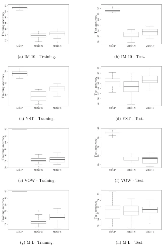
algo-rithms on IM-10, YST, VOW and M-L datasets. . . 37 4.4 Comparison between last generation individuals’ accuracies ofM3GP,M3GP-N
and M3GP-S algorithms on Heart, IM-3, WAV and SEG datasets. . . 38 4.5 Comparison between last generation individuals’ accuracies ofM3GP,M3GP-N
and M3GP-S algorithms on IM-10, YST, VOW and M-L datasets. . . 39
5.1 Toy example of the functioning of gsi-mutation applied to a 2-dimensional individual, and a dataset with 3 classes and 38 training samples. . . 43 5.2 Peak functions with different values of σ2
i: the green has σi2=0.1, the orange has σ2i=0.05 and the blue has σi2=0.01. . . 47
5.3 The same toy example as in figure 5.1, of a 2-dimensional individual and a dataset of 3 classes. The moving point is a randomly chosen point from inside the grey rectangle. . . 54 5.4 A 2-dimensional hyperellipse and the 2-dimensional hyperrectangle with sides
alligned with the hyperellipse axes and diagonals’ intersection equal to the hy-perellipse centroid. . . 56
LIST OF FIGURES xvii
5.5 Probability of a point generated inside the hyperrectangle to be inside the hy-perellipse, depending on the number of dimensions d. . . 57 5.6 Given the number of dimensions, d, Volume HR/Volume HE gives the minimum
number of points that have to be generated (inside the hyperrectangle) to find one inside the hyperellipse. . . 58 5.7 The 3σ-hyperrectangle for a 2-dimensional individual. . . 62 5.8 Comparison between median accuracies ofM3GP 50, Baseline 0.0001%Baseline
1% and Baseline 10% algorithms on HRT, IM-3, WAV and SEG datasets. . . 76 5.9 Comparison between median accuracies ofM3GP 50,Baseline 0.0001%,Baseline
1% and Baseline 10% algorithms on IM-10, YST, VOW and M-L datasets. . . . 77 5.10 Comparison between last generation individuals’ accuracies of M3GP 50,
Base-line 0.0001%, Baseline 1% and Baseline 10% algorithms on HRT, IM-3, WAV and SEG datasets. . . 78 5.11 Comparison between last generation individuals’ accuracies of M3GP 50,
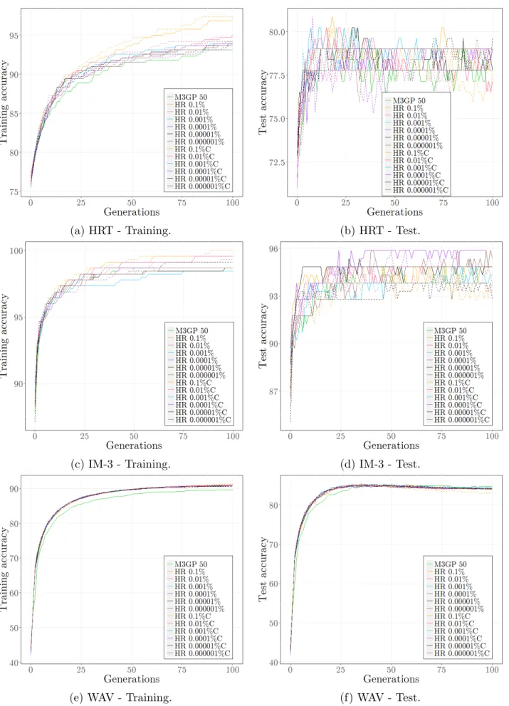
Base-line 0.0001%, Baseline 1% and Baseline 10% algorithms on IM-10, YST, VOW and M-L datasets. . . 79 5.12 Comparison between median accuracies of M3GP, HR 10k% and HR 10k%C
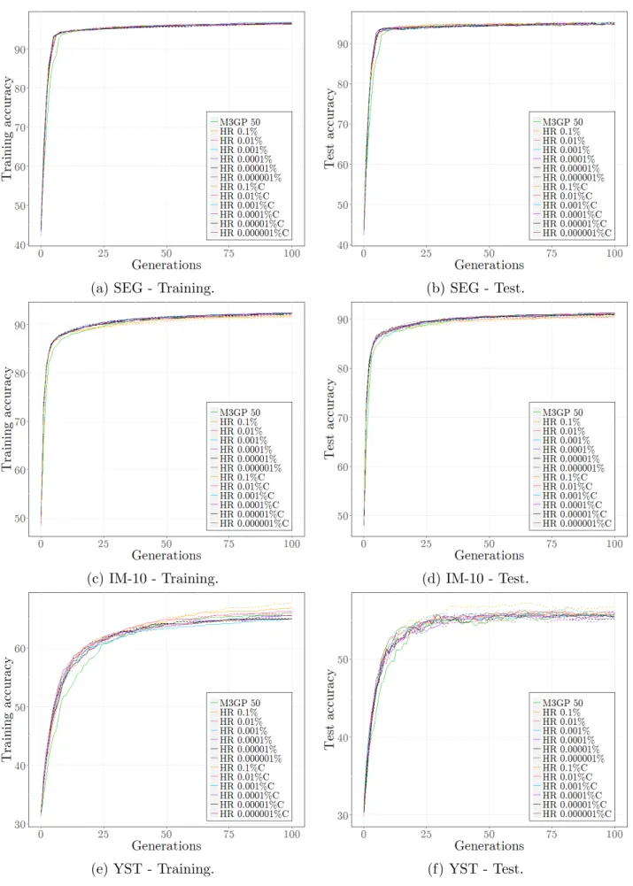
(dashed lines) algorithms, with k ∈ {−1, ..., −6}, on HRT, IM-3 and WAV datasets. 87 5.13 Comparison between median accuracies of M3GP, HR 10k% and HR 10k%C
(dashed lines) algorithms, with k ∈ {−1, ..., −6}, on SEG, IM-10 and YST datasets. 88 5.14 Comparison between median accuracies of M3GP, HR 10k% and HR 10k%C
(dashed lines) algorithms, with k ∈ {−1, ..., −6}, on VOW and M-L datasets. . . 89 5.15 Comparison between last generation individuals’ accuracies of M3GP, HR 10k%
and HR 10k%C algorithms, with k ∈ {−1, ..., −6}, on HRT, IM-3 and WAV datasets. . . 90 5.16 Comparison between last generation individuals’ accuracies of M3GP, HR 10k%
and HR 10k%C algorithms, with k ∈ {−1, ..., −6}, on SEG, IM-10 and YST datasets. . . 91
xviii LIST OF FIGURES
5.17 Comparison between last generation individuals’ accuracies of M3GP, HR 10k% and HR 10k%C algorithms, with k ∈ {−1, ..., −6}, on WAV and M-L datasets. . 92
5.18 Comparison between median accuracies of M3GP and the hyperrectangle vari-ants on HRT, IM-3 and WAV datasets. . . 96 5.19 Comparison between median accuracies of M3GP and the hyperrectangle
vari-ants on SEG, IM-10 and YST datasets. . . 97 5.20 Comparison between median accuracies of M3GP and the hyperrectangle
vari-ants on VOW and MOVL datasets. . . 98 5.21 Comparison between last generation individuals’ accuracies of M3GP 50 and the
hyperrectangle variants on Heart, IM-3 and WAV datasets. . . 99 5.22 Comparison between last generation individuals’ accuracies of M3GP 50 and the
hyperrectangle variants on SEG, IM-10 and YST datasets. . . 100 5.23 Comparison between last generation individuals’ accuracies of M3GP 50 and the
hyperrectangle variants on WAV and M-L datasets. . . 101 5.24 Comparison between median accuracies ofM3GP 50,HE χ225%,HE χ250% andHE
χ2
99% algorithms on HRT, IM-3, WAV and SEG datasets. . . 106 5.25 Comparison between median accuracies ofM3GP 50,HE χ2
25%,HE χ
2
50% andHE
χ299% algorithms on IM-10, YST, VOW and M-L datasets. . . 107 5.26 Comparison between last generation individuals’ accuracies of M3GP 50, HE
χ2
25%, HE χ250% and HE χ299% algorithms on HRT, IM-3, WAV and SEG datasets. 108
5.27 Comparison between last generation individuals’ accuracies of M3GP 50, HE χ2
25%, HE χ 2
50% and HE χ 2
99% algorithms on IM-10, YST, VOW and M-L datasets. 109
5.28 Comparison between median accuracies of M3GP 50, HE χ2
50% and HE χ299%
algorithms on HRT, IM-3, WAV and SEG datasets. . . 112 5.29 Comparison between median accuracies of M3GP 50, HE χ2
50% and HE χ
2 99% algorithms on IM-10, YST, VOW and M-L datasets. . . 113
5.30 Comparison between last generation individuals’ accuracies ofM3GP 50, HE χ250% and HE χ2
99% algorithms on HRT, IM-3, WAV and SEG datasets. . . 114
5.31 Comparison between last generation individuals’ accuracies of M3GP 50, HE χ250%, HE χ299% algorithms on IM-10, YST, VOW and M-L datasets. . . 115
5.32 Comparison between last generation individuals’ median accuracies of M3GP 50 and Donut algorithms on HRT, IM-3 WAV, SEG, IM-10, YST, VOW and M-L datasets. . . 119
5.33 Comparison between last generation individuals’ accuracies of M3GP 50 and MHR algorithms on WAV, SEG, IM-10 and M-L datasets. . . 122
5.34 Comparison between last generation individuals’ test accuracies of M3GP 50, MHE χ299% and MHE χ210% algorithms on IM-3, WAV, SEG, IM-10, YST and M-L datasets. . . 125
5.35 Comparison between last generation individuals’ accuracies of M3GP 50, AM0.5σ, AM1σ and AM2σ algorithms on HRT, IM-3, WAV, SEG, IM-10, YST, VOW and M-L datasets. . . 128
5.36 Comparison between last generation individuals’ accuracies of M3GP 50, AM10% and AM25% algorithms on HRT, IM-3, WAV, SEG, IM-10, YST and M-L datasets.131
5.37 Comparison between last generation individuals’ accuracies of M3GP 50, CMD AVG-A, CMD AVG-C, CMD MED-A and CMD MED-C algorithms on HRT, IM-3, WAV, SEG, IM-10, YST and M-L datasets. . . 135
5.38 Comparison between last generation individuals’ accuracies of M3GP 50, CMD MED-A 25% and CMD MED-A 100% algorithms on HRT, IM-3, WAV, SEG, IM-10, YST and M-L datasets. . . 138
6.1 Comparison between last generation individuals’ accuracies of M3GP 50, HR, HR-XO EP, HR-XO X&M, AM1σ, AM1σ-XO EP and AM1σ-XO X&M algo-rithms on HRT, IM-3, WAV and SEG datasets. . . 145
6.2 Comparison between last generation individuals’ accuracies of M3GP 50, HR, HR-XO EP, HR-XO X&M, AM1σ, AM1σ-XO EP and AM1σ-XO X&M algo-rithms on SEG, IM-10, YST and M-L datasets. . . 146
Chapter 1
Introduction
Genetic Programming (GP) is able to produce good and competitive results for regression problems and binary classification problems. However, in multiclass classification problems, GP is not able to achieve state-of-the-art performance[4]. In 2014, a new multiclass classification algorithm, able to achieve state-of-the-art performance, was proposed[8]. The algorithm is called Multidimensional Multiclass Genetic Programming (M2GP) and its name was chosen based on the fact that, at each iteration, a population of multidimensional solutions is created. In 2015, a new version of M2GP was introduced: Multidimensional Multiclass Classification Genetic Programming with Multidimensional Populations (M3GP)[15]. While in M2GP the number of dimensions of each solution is fixed, in M3GP the number of dimensions of each solution might differ from solution to solution. In both algorithms, GP is used as a feature extraction method, then a clustering procedure is applied and, finally, the Mahalanobis distance is used to measure the quality of the feature transformation[15].
Moraglio et al. proposed, in 2012, semantic aware genetic operators[14], i.e. genetic operators that are able to manipulate the syntax of the solutions in such a way that their effect on semantics is ”known”. These geometric semantic genetic operators are able to outperform the traditional genetic programming operators, although they might produce more complex and bigger solutions.
2 Chapter 1. Introduction
The motivation for this thesis comes from the powerful properties of geometric semantic genetic operators and the interesting approach used by M2GP and M3GP to solve multiclass classification problems. The main ambition was to create an operator to M3GP, inspired in the geometric semantic operators, able to change the classification of specific instances without changing the classification of the others. This operator is called geometric semantic inspired mutation and it is integrated in a new multiclass classification algorithm - Geometric Semantic Inspired M3GP (in short, GSI-M3GP).
The document is organized as follows. Chapter 2 introduces the reader to Machine Learning, to Evolutionary Algorithms and to two multiclass classification algorithms which are the base of this thesis’ work: the previously referred M2GP and M3GP. Chapter 3 comprises the original results of M3GP using the MATLAB original implementation[15, 17] and the results obtained with a different implementation, a Java implementation, developed in the context of this thesis. In Chapter 4, the Euclidean and Mahalanobis distance measures are discussed and the results of general changes to M3GP are presented. Chapter 5 presents the new genetic operator and hence, the new multiclass classification algorithm - Geometric Semantic Inspired M3GP. Different versions of the new algorithm are described and the results are also presented. Chapter 6 introduces a slight variation of the classification algorithm presented in Chapter 5, by adding a crossover operator to the set of genetic operators. Chapter 7 briefly highlights the main implementation issues of M3GP. Finally, Chapter 8 closes this document with a summary of contributions, what could have been done differently and what can still be improved in the future.
Chapter 2
Background Theory
2.1
Machine Learning
Machine Learning is the area of Artificial Intelligence which studies the construction of computer programs/algorithms that learn/improve by means of experience in an automatic way[13]. The learning process of a machine learning algorithm is done using data and, after that, some algorithms are used to make predictions on new data.
The data used by the algorithms in the learning process can be represented in the following format: x1 x2 x3 ... xp x11 x12 x13 ... x1p x21 x22 x23 ... x2p ... ... ... ... ... xm1 xm2 xm3 ... xmp t t1 t2 ... tm
i.e. as a m × p matrix, where each line represents an instance and each column represents a variable, and additionally, a m-dimensional vector might also be given. Variables x1 to xp are
4 Chapter 2. Background Theory
called features and variable t is the target variable. When a target variable exists, then the objective of the algorithm is to, based on the p-dimensional instances, predict the values in t.
Machine Learning tasks can be classified according to whether a target variable exists (i.e. if data is labelled) and, in that case, also according to its type. If all data is labelled, then we are in the presence of a Supervised Learning problem. If data is not labelled, we have, depending on the purpose, an Unsupervised Learning problem or a Reinforcement Learning problem. If a target variable exists but not all data is labelled, then we are in the presence of a Semi-Supervised problem.
2.1.1
Supervised Learning
Supervised Learning problems can be further divided into Classification and Regres-sion problems. In a Classification problem, an instance is classified as belonging to a certain group/class and this class can be represented by an integer. When the target variable is con-tinuous, then the problem is a Regression problem.
2.2
Evolutionary Algorithms
Evolutionary Algorithms (EAs) are a family of heuristic population-based optimization algorithms inspired in biological evolution. These algorithms are heuristic since their solutions are created in a way that they are sufficiently good, but the global optimal solution is not necessarily found.
EAs are inspired by biological evolution since they use Charles Darwin’s concepts of repro-duction, likelihood of survival, variation, inheritance and competition[5, 18]. As such, instead of creating only one solution that, hopefully, improves from iteration to iteration, a family of solutions (a population) is created so that the previously referred biological concepts can be applied. Also, instead of iteration, the word generation is used.
2.2. Evolutionary Algorithms 5
Genetic Programming is one of the existing types of EAs.
2.2.1
Genetic Programming
Genetic Programming (GP)[11] was presented by John Koza in 1992 and, as an evo-lutionary algorithm, it evolves a population of computer programs[16]. An initial population of programs (individuals, in GP terms) is created and, at each generation, genetic operators are applied to the best individuals of the previous population, creating new individuals which might be better than the previous ones. More thoroughly, the basic steps of the GP algorithm are described bellow:
1. Randomly generate an initial population of individuals, P ;
2. Evaluate the individuals’ fitness;
3. Repeat for a predefined number of generations or until another termination condition is met:
(a) Create an empty population P0;
(b) Repeat until the number of individuals in P0 is equal to the number of individuals in P :
i. Select one or two individuals from P , with probability of selection based on fitness;
ii. Apply one of the genetic operators (with specified probabilities) to the selected individuals to create new individuals;
iii. Add the previously created individuals to the new population P0;
(c) Evaluate the individuals in P0;
(d) Set P = P0.
6 Chapter 2. Background Theory
The concepts of fitness, selection and genetic operators are now going to be explained. It will also be explained what a program/individual really is, its characteristics, how it is represented and the methods used to generate it.
Individuals Representation
In GP, programs or individuals are solutions for the considered problem, and they can be represented in various different ways. One of the most commonly used is the tree structure, as shown in figure 2.1. / 0 + 1 3 4 x2 2 x1 3 Figure 2.1: GP program/individual.
The individual represented in figure 2.1 is the function f (x1, x2) = (x2+ x1) ÷ 3, where x1 and x2 are features of the dataset. The individual might also be represented as
(/ ( + ( x2 x1) 3)
i.e. in the called prefix notation[16] (always from left to right, as the numbers in figure 2.1 imply). The inspiration for the prefix notation comes from Lisp programming language[11]. This notation is useful since it makes it easy to access subtrees of the tree representing the individual.
To construct an individual, two sets are considered: the function set and the terminal set. The function set is the set of functions or arithmetic operators, F = {f1, ..., fl} (with l ∈ Z),
2.2. Evolutionary Algorithms 7
and these are present in the trees as internal nodes. The terminal set consists of features and constant values, T = {t1, ..., tj} (with j ∈ Z), which appear as leaf nodes of the trees.
One can consider that the tree in figure 2.1 was created considering, for example, the function set F = {+, −, ×, ÷} and the terminal set T = {0, ±1, ±2, ±3} ∪ {x1, x2, x3}.
Each node of the tree has a depth value associated to it, which corresponds to the number of edges from the root node to it. The root node corresponds to the first node to write in the prefix notation (or to the node in the ”highest” position when drawing the tree).
The tree itself has a depth value associated to it, and it corresponds to the depth of the deepest node in the tree. As an example, the tree represented in figure 2.1 has a depth of 2.
Methods to generate GP individuals,[11]
The individuals in the initial population are created using one of the following three known methods (and specifying the maximum depth):
• Full method:
Trees created using Full always have depth value equal to the maximum depth. While the maximum depth is not reached, nodes are taken at random from the function set. Nodes at depth equal to the maximum depth are randomly chosen from the terminal set. This method produces very regular trees, as the one in figure 2.2.
+ 0 -1 × x2 2 x3 2 x1
Figure 2.2: Example of a GP individual created using method Full, with maximum depth equal to two.
8 Chapter 2. Background Theory
• Grow method:
Grow produces trees which have depth smaller or equal to the predefined maximum. Each node with depth smaller than the predefined maximum is randomly chosen from T ∪ F , so it can be a function or a terminal. If the predefined maximum depth is reached, then nodes with that depth are taken from T . Thus, this method produces very irregular trees, as the ones in figure 2.3, which have depth of two, one and zero, respectively.
/ 0 2 1 + x2 2 x3 -1 x3 x1
Figure 2.3: Examples of GP individuals created using method Grow, with maximum depth equal to two. From left to right, the trees have, respectively, depth of 2, 1 and 0.
• Ramped half-and-half method:
When using Ramped half-and-half initialization method, the number of individuals is divided by the maximum depth value, so that an equal percentage of individuals is created with each value of depth between 1 and the maximum depth. Then, for each value of depth, half of the individuals are created using Full and the other half is created using Grow. This way, the initial population is composed of individuals of different sizes and shapes.
As an example, if a population is composed of 100 individuals and the maximum depth is 5, then 20% of the individuals will have depth 1, 20% will have depth 2, and so on.
Fitness evaluation of the individuals
GP is an optimization algorithm, so the solutions it produces need to be evaluated. Fitness measures how good a solution is, i.e. how close it is to the global optimum solution. The name fitness is used because of GP’s Darwinism inspiration.
2.2. Evolutionary Algorithms 9
A fitness function is defined and used to evaluate individuals, so that they can be compared between each other. Examples of fitness functions are the sum of absolute errors (used for regression problems) and accuracy (used in classification problems). If considering the sum of absolute errors then the purpose of the optimization problem is to minimize it. When using accuracy, one is optimizing by maximizing accuracy.
Selection
Selection is another biological evolution inspiration. In nature, individuals compete and the best individuals have a higher probability to be chosen for mating. In GP, selection methods are probabilistic methods used to select individuals. One of the most used is the tournament selection method [11, 16].
Tournament selection method: Each time an individual needs to be selected, a tourna-ment is performed. A prefixed number of individuals is randomly chosen from the population, with repetition allowed. Then, the individual in the tournament which has the best value of fitness is selected.
Genetic operators
Genetic operators are used to create a new population of individuals given a previous existing population. The crossover operator mimics sexual reproduction and mutation mimics the fact that each individual, besides having parents’ characteristics, also has characteristics of its own that cannot be found in any of the parents.
• Standard GP Crossover is a binary operator, needing two individuals to be performed. Two individuals are selected using a selection method. These individuals are called parent individuals. Crossover starts by first selecting a crossover point in each of the parents. These crossover points are randomly and independently selected and correspond to one of the nodes in each parents’ tree. Two offspring individuals (the resulting individuals
10 Chapter 2. Background Theory
from applying the crossover operator) are created by exchanging the subtrees with root at the crossover points. An example can be found in figure 2.4.
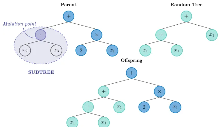
• Standard GP Mutation can be seen as a unary operator, as it only needs one parent individual to be performed. But it can also be interpreted as a binary operator since, besides needing a parent individual, it also needs a random tree in order to be performed. The parent individual is selected using a selection method. A node from the parent is chosen at random and with discrete uniform distribution, to be the mutation point. The subtree with root at the mutation point, i.e. the subtree below the mutation point, is replaced by a new tree - a tree which is randomly generated using Full or Grow. Figure 2.5 is an example of applying the mutation operator.
+ Parent #1 - × 1st SUBTREE x2 x3 2 x1 Crossover point / Parent #2 2 + Crossover point x2 x3 2nd SUBTREE + Offspring #1 - × x2 x3 2 + x3 x2 / Offspring #2 2 x1
2.2. Evolutionary Algorithms 11 + Parent -Mutation point × SUBTREE x2 x3 2 x1 + Random Tree x1 + x1 x1 + Offspring + + x1 x1 x1 × 2 x1
Figure 2.5: Example of an individual generated by the mutation operator. The random tree was generated using grow.
2.2.2
Geometric Semantic Genetic Programming (GSGP)
The semantics of a GP individual can be defined as the m-dimensional point of outputs of the individual on the input data[14, 18]. Mathematically, the semantics of an individual P is given by
SP = (P ( ~y1), ..., P ( ~ym)),
where ~yi is the ith instance, with i ∈ {1, ..., m}, of the given dataset.
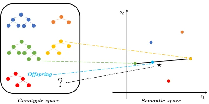
Considering a population of individuals, each of the individuals’ semantics can be represented as a point in a m-dimensional space. The target variable can also be represented in this space. While one knows the semantics of an individual by knowing its corresponding tree, one does not necessarily knows which tree corresponds to the point representing the target (see figure 2.6). If that was the case, then the considered optimization problem would be solved[18].
12 Chapter 2. Background Theory
Figure 2.6: Representation of the genotypic space (where individuals are represented by their trees) versus the semantic space (where the individuals are represented by their semantics). The semantic space is 2-dimensional since one is considering a toy example of a dataset with only 2 instances. The star corresponds to the target.
In 2012, Moraglio et al. presented two operators that act on the semantics of the individuals, transforming the fitness landscape, making it unimodal. When a unimodal fitness landscape is considered, no local optima exists, only the global optimum. This means that there is always chance of improvement. These operators are called Geometric Semantic Crossover (GSC) and Geometric Semantic Mutation (GSM)[14].
While individuals created using standard GP genetic operators have semantics anywhere in the semantic space (and not necessarily close to the semantics of the parents), one knows where the semantics of the individuals created using the geometric semantic operators are, relatively to their parents’ semantics. If GSM is applied to an individual, the semantics of the offspring is around the parent semantics (see figure 2.7). When GSC is applied, the semantics of the offspring is between the parents’ semantics (see figure 2.8).
2.2. Evolutionary Algorithms 13
Figure 2.7: Toy example of the application of the geometric semantic mutation. T1, T2,...,T6 is a sequence of trees to which the geometric semantic mutation is applied, where Ti+1 is generated by applying the operator to Ti. By generating a tree using the mutation operator, the semantics of the offspring is inside a grey square (since the semantic space is 2-dimensional, because one is considering a dataset with 2 instances) with center in the semantics of the parents. There is always a chance of improvement, as expressed here. The star represents que target.
Figure 2.8: Example of applying the geometric semantic crossover operator to two parent trees. The offspring has semantics falling in the line segment joining the semantics of the parents, so the offspring might be closer to the target - the offspring is not worse than the worst of the parents. The semantic space is bi-dimensional since a 2 instance dataset is being considered, for simplicity. The star represents the target.
14 Chapter 2. Background Theory
The big disadvantage of GSGP is that the individuals created by GSC and GSM are always bigger than their parents and so, from generation to generation, the individuals grow very quickly[6], making GSGP impossible to use in some cases. In 2013, a new implementation was proposed[19], for which not all the individuals had to be stored, only their semantics, making GSGP able to be used.
Geometic semantic operators
• Geometric Semantic Crossover
Let P1, P2 : Rp −→ R be two parent individuals, chosen using a selection method (de-scribed in the previous subsection). The offspring individual, OXO : Rp −→ R, is the following:
OXO = P1× R + P2 × (1 − R),
where R is a randomly generated tree with output values in [0,1]. • Geometric Semantic Mutation
Let P be the parent individual, P : Rp −→ R, chosen using a selection method. The offspring individual, OM : Rp −→ R, is the following:
OM = P + ms × (R1− R2),
where R1 and R2 are randomly generated trees, and ms is a predefined real number called mutation step.
2.3
Multiclass classification problems and algorithms
Let us consider a dataset D with m instances and p features. This can be represented by a m × p matrix. Let us also consider a vector ~t ∈ Rm (the target variable values), and the set of classes C = {1, 2, ..., c}.
2.3. Multiclass classification problems and algorithms 15
Each one of the m p-dimensional instances of D belongs to one of the classes in C. The ith instance belongs to the class stored in the ith entry of ~t.
Let us consider a partition of dataset D in two datasets: the training set and the test set. The training set (D|T, with n instances) is the set of instances used to create solutions/models, and the test set (D|U, with m-n instances) is the set used to check the models’ generalization ability. The models are created in such a way that the accuracy of predictions is maximized (or, equivalently, another metric might be used). However, the model needs to generalize well on unseen data. That is, the model also needs to be able to predict accurately the class to which an unseen instance belongs. If that happens, the model has generalization ability. Otherwise, it overfits training data, i.e. it just ”mimics” training data.
Given a new instance ~y ∈ Rp, to which class does ~y belong to? A classification algorithm solves this problem by, based on data in D, finding a function f : Rp −→ C, i.e. a function that assigns a class to a given instance, and so by applying f to ~y one gets f (~y) = a ∈ C.
2.3.1
Multidimensional multiclass Genetic Programming (M2GP)
In 2014, Ingalalli et al. presented a new multiclass classification algorithm called Multidi-mensional Multiclass Genetic Programming[8] (from now on M2GP).
In M2GP, GP is used as a wrapper method. That is, GP is used as a feature extraction method, transforming the original set of p variables in a new set of d variables. The quality of this transformation is then evaluated by a predefined measure[15].
Thus, two steps are considered:
1. Creation of a d -dimensional tree: g : Rp −→ Rd, d ≥ 1;
16 Chapter 2. Background Theory
GP typically transforms a set of p variables in only one variable. This is not considered informative enough in muticlass classification[8]. Therefore, instead of having a typical GP tree, M2GP creates trees with d dimensions (also called branches in M2GP terms), where d ≥ 1.
Figure 2.9 presents possible multidimensional trees. Variables x1 and x2 are 2 of the p features in the dataset. The blue squared nodes are the root nodes of each one of the trees. In multidimensional trees, the root node exists just to define the number of dimensions of the tree. + x1 x2 + x1 x2 / x1 4
Figure 2.9: Example of a one-dimensional tree and a two-dimensional tree.
It is important to notice that the number of dimensions, d, is a parameter of the algorithm and so, it does not depend on the number of classes/features/etc.
Applying function g to each one of the n training instances, one gets n d -dimensional points that can be represented in a d -dimensional space. Let us refer to these points as the mapped training instances. The mapped training instances are then clustered according to the classes in C, and classified using function h.
The fact that GP is only used as a wrapper method, implies that an M2GP solution does not consist only of the tree, but also of other structures that are used in the evaluation of the individual[8].
2.3. Multiclass classification problems and algorithms 17
Applying g to the m − n test instances in D, one gets a (m − n) × d matrix called, from now on, mapped test instances. The previously mentioned evaluation structures are used to evaluate these outputs and assign a class to each one of the test instances.
M2GP algorithm - Training phase
Let:
• D|T refer to the set of n × p training instances in D;
• ~t |T refer to the n dimensional vector of training target values;
• d be a predefined number representing the number of dimensions of the trees; • C = {1, ..., c} be the set of classes in which instances can be grouped;
be the inputs of the training phase of M2GP algorithm.
Then, the pseudo-code of each generation’s training phase of the algorithm[8] is organized below:
1. C reate an empty population P .
2. Repeat until there are pop elements in P :
(a) Generate a d -dimensional tree, Pi, i ∈ {1, ..., pop}, using a genetic operator ;
(b) Evaluate Pi on D|T getting the matrix M T , the matrix of mapped training instances of Pi;
(c) Add the jth line in M T to Zk if ~t |jT= k, ∀j ∈ {1, ..., n}, where ~t |jT is the jth entry of ~t |T;
(d) For k ∈ C:
18 Chapter 2. Background Theory
ii. Create Mk= centroid(Zk); iii. Calculate Dk j = q (M Tj− Mk)TCk−1(M Tj − Mk), ∀j ∈ {1, ..., n}, where M Tj is the jth line of M T ; (e) For j ∈ {1, ..., n}
i. P redj = k, where k ∈ C such that Djk = min{D1j, ..., Djc}
ii. M atchedj = 1 ~t |jT= P redj 0 ~t |jT6= P redj
(f) Evaluate the training fitness of Ii: fT(Ii) = n1 Pn
j=1M atchedj. (g) Add individual Ii = (Pi, C1, ..., Cc, M1, ..., Mc) to the population.
Initial population
The trees in the initial population of M2GP are created in the same way as for GP - using Full, Grow or Ramped half-and-half methods. The only difference here is that the trees created for M2GP are d -dimensional and the root node is not a ”real” node, but the node defining the number of dimensions. The results presented in [8] were ran using Ramped half-and-half with 75% Full and 25% Grow.
Genetic operators
The genetic operators are also the same as the ones used in GP: mutation and crossover. The only restriction in M2GP is that the root node cannot be chosen as mutation/crossover point.
Calculation of the mapped instances
As previously referred, by applying the tree to an instance of D|T, one gets a d -dimensional point. Considering all the instances in D|T, the mapped training instances are considered as points in the d -dimensional, and grouped in clusters.
2.3. Multiclass classification problems and algorithms 19
Clustering
The clustering phase consists of grouping the mapped training instances according to the class to which the training instances belong. That is, the mapped training instances are divided in c groups (and c matrices are created, one corresponding to each class). According to the pseudo-code in page 15 and 16, these matrices are called Zk, with k ∈ {1, ..., c}.
Covariance matrices, centroids and Mahalanobis distance
For each one of the Zk matrices, a covariance matrix, Ck= covariance(Zk), and a centroid, Mk = centroid(Zk), are created. The entry (a, b) of Ck stores the covariance between column a and column b of Zk. Hence, each Zk matrix is d × d. The size of Mk = centroid(Zk) is d, and entry a of Mk (with a ≤ d) stores the average of Zk’s ath column.
M2GP is a classification algorithm. As such, it classifies instances into classes, i.e. it makes predictions. In M2GP the predicted values are found with the help of the covariance matrices and the centroids. The distances between the mapped training instances and all the centroids are considered. Each instance is assigned with the class for which the distance from the mapped training instance to the classe’s centroid is minimized. Thus, each instance is assigned with the class represented by that centroid.
The question is, why are the covariance matrices needed? The covariance matrices are needed because the Mahalanobis distance measure is the distance measure considered. In [8] two dis-tance measures are compared: the Euclidean and the Mahalanobis disdis-tance measures. Accord-ing to the authors, ”the distance measure indeed plays a significant role in the performance of M2GP” and, by using the Mahalanobis distance, M2GP is able to reach significantly better results.
The Mahalanobis distance between an observation x = (x1, ..., xd) and a set of samples characterized by a mean point µ = (µ1, ..., µd) and a covariance matrix Sd×d is given by:
20 Chapter 2. Background Theory
dM(x) =p(x − µ)TS−1(x − µ)
It is important to notice that, by using the Mahalanobis distance, one takes into consideration the correlations between variables. That is, the Mahalanobis distance assumes that variables are correlated and gives less importance to the variables with higher variances and to groups of variables with high correlations. When using the Euclidean distance, one assumes that variables are uncorrelated and have equal variance[10]. This topic will be addressed again in chapter 4.
Finally, looking at the Mahalanobis distance formula, one can see that it requires the calcu-lation of the inverse of S. As such, it is only possible to calculate the Mahalanobis distance if the covariance matrix is nonsingular.
Fitness function
The fitness function is the accuracy of the classification: the fraction or, equivalently, the percentage of correctly classified instances (as described in step 2.(f) of the algorithm in page 16).
Accuracy = Number of correctly classified instances Total number of instances
What is an individual?
Unlike GP, an M2GP individual consists not only of the function tree, but also, the covari-ance matrices and the centroids, as described in step 2.(g) of the training phase algorithm in page 16).
Testing phase
2.3. Multiclass classification problems and algorithms 21
• D|U refer to the set of (m − n) × p test instances in D;
• ~t |U refer to the m − n dimensional vector of test target values;
• d a predefined number representing the number of dimensions of the trees; • C = {1, ..., c} be the set of classes in which instances can be grouped;
• P a population of pop individuals - where each individual is composed by its tree, Pi, and the corresponding covariance matrices (C1,...,Cc) and centroids (M1,...,Mc).
be the inputs of the testing phase of M2GP algorithm.
Then, the pseudo-code of each generation’s testing phase of the algorithm[8] is organized below:
1. For each individual, Ii ∈ P (with i ∈ {1, ..., pop}):
(a) Evaluate Pi on D|U getting the matrix M U , the matrix of mapped test instances of Pi; (b) For k ∈ C: i. Calculate Dk j = q (M Uj − Mk)TCk−1(M Uj − Mk), ∀j ∈ {1, ..., m − n}, where M Uj is the jth line of M U ; (c) For j ∈ {1, ..., m − n}
i. P redj = h, where h ∈ C such that Djh = min{D1j, ..., Djc}
ii. M atchedj = 1 ~t |jU= P redj 0 ~t |jU6= P redj
(d) Evaluate the test fitness of Ii: fU(Ii) = m−n1
Pm−n
j=1 M atchedj.
The most important thing to refer is that, when classifying test data, the covariance matrices and the centroids are not recalculated.
22 Chapter 2. Background Theory
Trees’ number of branches, d
The main drawback of M2GP is that the number of dimensions is not automatically chosen, it is a parameter. And as a parameter, some questions can be posed, such as: what is its best value? Does this value change along the generations? Does it change from problem to problem?
The authors introduce, in [8], an automatic procedure to choose the number of dimensions. The procedure consists of creating initial populations with increasing values of d, while the accuracy of those populations increases. The procedure stops when the accuracy decreases. The chosen value of d is the last value for which the accuracy of the initial population increased. As such, d depends on the considered dataset.
2.3.2
M2GP with Multidimensional Populations (M3GP)
In 2015, Delgado et al. presented an improved version of M2GP, called Multidimensional Multiclass Genetic Programming with Multidimensional Populations or M2GP with Multidimensional Populations (in short, M3GP)[15].
The main drawback of M2GP pointed out by Delgado et al. is the fact the the number of dimensions is a parameter and its value is set before running the algorithm. M3GP does not have the number of dimensions as a parameter fixed before running the algorithm. M3GP evolves it with the algorithm.
Initial population
The initial population is composed by one-dimensional individuals. These individuals are created using Full method[11] with depth of 6.
2.3. Multiclass classification problems and algorithms 23
Genetic operators
The genetic operators used to create individuals in M3GP are different from the ones con-sidered in M2GP. Mutation and crossover can be chosen to create a new individual with equal probability.
If Mutation is chosen, one of the following operators is randomly chosen, with equal proba-bility:
• Standard subtree mutation: a mutation point is randomly selected (excluding the root node) and the subtree below the mutation point is replaced by a randomly created tree;
• Add new dimension: a randomly created new branch is added to the tree, i.e. a one-dimensional tree is added as a branch of the parent’s tree.
• Remove existing dimension: a branch of the tree is randomly selected to be removed from the tree;
If Crossover is chosen, one of the following two operators is applied, both having the same probability of being chosen:
• Standard subtree crossover: two crossover points are randomly and independently selected (excluding the root node) from two parent trees and the subtrees below the points are interchanged;
• Swap dimensions: A randomly chosen dimension from a parent tree is replaced by a randomly chosen dimension from another parent’s tree;
Hence, Mutation is responsible by increasing and decreasing the number of dimensions of the individual.
24 Chapter 2. Background Theory
Pruning procedure
As just referred, Mutation is responsible for adding and removing dimensions to the indi-viduals. However, as expressed in [15], an excessive number of dimensions might decrease the accuracy and, on the other side, the remove dimensions’ operator removes a random branch, which might also decrease accuracy. Because of this fact, the authors say that the remove dimensions’ operator is ”blind to fitness”.
The pruning procedure was created to counteract this problem and it is applied, at each generation, to the tree corresponding to the individual with higher training accuracy in the population. Let T represent that tree. The pseudo-code for the pruning procedure is:
1. Let d be the number of dimensions of T ; 2. Set i := 1;
3. Repeat while i ≤ d:
(a) Let T0 be the tree found by removing the ith dimension of T ;
(b) If Training Accuracy(T0)>Training Accuracy(T ) Then:
i. Set T := T0;
(c) Else:
i. Increment the value of i ; 4. Return T .
Chapter 3
M3GP algorithm original results
As referred in section 2.3.2, M3GP was first presented in 2015 by Delgado et al.[15], and a modified version of GPLAB 3 (an open source GP toolbox for MATLAB, available in http://gplab.sourceforge.net)[17] was used to get all the results.
The results presented in this document were obtained using a new implementation developed in the context of this thesis - a Java implementation.
3.1
Experimental setup and results
M3GP was originally run on 8 problems, i.e. on 8 datasets with varying number of classes, attributes and samples (see table 3.1). These are the problems which are going to be considered for this experimental analysis (and also in the following chapters).
Dataset HRT IM-3 WAV SEG IM-10 YST VOW M-L
# classes 2 3 3 7 10 10 11 15
# attributes 13 6 40 19 6 8 13 90
# samples 270 322 5000 2310 6798 1484 990 360 Table 3.1: Description of the datasets used for the experimental analysis.
26 Chapter 3. M3GP algorithm original results
Datasets HRT, SEG, YST, VOW and M-L can be found at the KEEL dataset repository[2], while IM-3 and IM-10 are the satellite datasets used in [1] and WAV can be found in [3].
Each of these datasets is of the following format:
x1 x2 x3 ... xp t x11 x12 x13 ... x1p t1 x21 x22 x23 ... x2p t2 ... ... ... ... ... ... xm1 xm2 xm3 ... xmp tm
where p is the number of attributes and m is the number of samples, and so each of the lines in the dataset is a sample. The last column of each dataset is the target variable, the variable with the values to predict.
The following table (table 3.2) presents the running parameters of the original M3GP[15], which we are leaving unchanged in the first subsection, to have a fair comparison between the two implementations.
Runs 30
Population size 500 individuals Generations 100 generations
Initialization 6-depth Full Initialization[11]
Operator probabilities Crossover pc = 0.5, Mutation pµ = 0.5 Function set +, -, ×, ÷ protected as in [11]
Terminal set Ephemeral random constants [0,1] Bloat control 17-depth limit[11]
Selection Lexicographic tournament[12] of size 5 Elitism Keep best individual
Table 3.2: Running parameters of M3GP.
For each run of the algorithm on a specific dataset, the dataset is randomly split into training and test sets: 70% of samples for training and the remaining 30% for test (more specifically, the samples were shuffled and then the partition was made).
3.1. Experimental setup and results 27
The comparisons between algorithms/versions are presented in terms of training accuracy, test accuracy and number of nodes. Additionally, the number of dimensions is presented. Notice that the number of dimensions is only informative, as a bigger number of dimensions does not imply that the individual has more nodes.
Two results are said to be significantly different (throughout all the document), when their difference is statistically significant according to the Wilcoxon’s rank sum test considering a significance level of 1% (0.01).
3.1.1
Original results
This subsection presents a comparison between the original results of M3GP (obtained using GPLAB toolbox[17]) and the results obtained with the Java implementation.
As expected, there are no discrepancies between the results obtained with the original imple-mentation of M3GP using the GPLAB toolbox from MATLAB and the new Java implementa-tion.
HRT IM-3 WAV SEG IM-10 YST VOW M-L Training accuracy M3GP original[15] 94.7 99.6 90.7 98.1 93.0 68.5 100 100 M3GP new 95.0(2.6) 99.6(0.4) 90.8(0.4) 98.1(0.4) 93.3(0.4) 69.1(1.2) 100(0.0) 100(0.0) Test accuracy M3GP original 79.0 95.4 84.3 95.6 91.0 56.3 93.8 57.1 M3GP new 79.0(4.5) 95.9(2.5) 84.0(0.9) 95.7(0.8) 91.3(0.7) 56.6(2.0) 95.5(1.9) 62.5(7.4) # of nodes M3GP original 110 66 71 111 239 274 53 13 M3GP new 318(45-422) 66(35-701) 132(39-213) 367(62-367) 777(261-1283) 317(203-888) 42(42-72) 11(11-209) # of dimensions M3GP original 12(1-17) 5(2-8) 31(29-37) 11(5-21) 12(11-16) 13(11-18) 20(16-20) 12(10-13) M3GP new 13(3-26) 5(3-13) 34.5(25-38) 11.5(5-17) 17(10-21) 14(11-22) 23(20-24) 11(8-13)
Table 3.3: Comparison between the original[15, 17] and new implementation of M3GP.
Table 3.3 presents results of training accuracy and test accuracy that refer to a median of 30 runs, and in parenthesis the standard deviation (for the new implementation). There is also information regarding the number of nodes: for M3GP original the number of nodes of the best individual; for M3GP new the number of nodes of the best individual and, in parenthesis, the
28 Chapter 3. M3GP algorithm original results
mininum and maximum number of nodes obtained on the 30 runs. Additionally, the median number of dimensions and, in parenthesis, the minimum and maximum number of dimensions.
3.1.2
M3GP with a smaller population
In the original version of M3GP[15], the population size was set to 500 individuals. Per generation, {500 × #Classes} cluster centroids, {500 × #Classes} covariance matrices are created. For each invertible matrix its inverse is also created. This is a process which might take a lot of time (which depends on the dataset, on the implementation and on the machine used to run the algorithm), if the number of classes or the number of samples is high.
Therefore, here M3GP is ran setting the population size to 50 (while the remaining parameters of table 3.2 are left unchanged), and compared to the algorithm ran with 500 individuals. The results are stored in table 3.4. The values in bold represent the best version (between M3GP 500 and M3GP 50 ), regarding training accuracy and test accuracy. When the difference is not statistically significant, both values are marked in bold.
HRT IM-3 WAV SEG IM-10 YST VOW M-L Training accuracy M3GP 500 95.0(2.6) 99.6(0.4) 90.8(0.4) 98.1(0.4) 93.3(0.4) 69.1(1.2) 100(0.0) 100(0.0) M3GP 50 93.1(3.2) 98.7(0.6) 89.6(0.6) 96.4(0.7) 92.3(0.8) 66.0(5.0) 100(0.0) 100(0.6) Test accuracy M3GP 500 79.0(4.5) 95.9(2.5) 84.0(0.9) 95.7(0.8) 91.3(0.7) 56.6(2.0) 95.5(1.9) 62.5(7.4) M3GP 50 77.8(4.0) 94.3(2.6) 84.7(0.9) 95.1(1.0) 91.1(0.9) 55.6(3.8) 94.3(2.3) 60.6(5.9) # of nodes M3GP 500 318(45-422) 66(35-701) 132(39-213) 367(62-367) 777(261-1283) 317(203-888) 42(42-72) 11(11-209) M3GP 50 176(45-359) 542(39-542) 42(20-177) 73(20-279) 258(85-818) 560(78-573) 45(45-111) 12(12-163) # of dimensions M3GP 500 13(3-26) 5(3-13) 34.5(25-38) 11.5(5-17) 17(10-21) 14(11-22) 23(20-24) 11(8-13) M3GP 50 14(1-19) 5.5(2-10) 26.5(20-32) 8(5-14) 15(8-24) 12(2-17) 22(19-25) 11(8-12)
Table 3.4: Comparison between M3GP with 500 individuals and 50 individuals.
Regarding training accuracy, M3GP 500 is always significantly better than M3GP 50 on all the problems (except for VOW and M-L, for which the median values are equal). Test accuracy was not significantly distinct between the two versions on all the datasets except for SEG and WAV datasets: for SEG, the version with 500 individuals was better in terms of test accuracy; for WAV, test accuracy was better setting the population size to 50 individuals.
3.1. Experimental setup and results 29
Regarding number of nodes, the range of values (max − min) is always smaller when the population size is 50 (except for VOW dataset).
Given that running M3GP with a population of 50 individuals instead of 500 is much quicker (since it requires the computation of 10 times less individuals) and there is no statistical dif-ference between the test values (except for SEG and WAV dataset, and for WAV it is better to have 50 individuals), in chapters 5 and 6 the experimental analysis is performed setting the population size to 50.
Chapter 4
General changes to M3GP
The use of the Mahalanobis distance can be seen as a disadvantage of M3GP, since it requires the computation of big matrices (although symmetric) and their inverses. Previous versions of the algorithm used the Euclidean distance, but the solutions were significantly worse (in terms of accuracy) than the ones found using the Mahalanobis distance[8]. Although, in our daily life, we are used to the Euclidean distance, by using it we assume that[10]:
• all variables have the same variance;
• variables are uncorrelated;
This is something that does not happen in M3GP, more specifically, it does not happen with the branches/dimensions of an M3GP solution/individual. Each branch is a variable, from now on referred to as wi. These wi variables are functions of the original features present in the dataset.
To better understand this, one can take a look at the tree in figure 4.1, which is a possible M3GP solution. There are two dimensions: w1(x1, .., xp) = x1and w2(x1, .., xp) = 0.01x1(where xi, i ∈ {1, ..., p}, are the feature variables of the dataset).
4.1. M3GP-N: Min-Max Normalization 31
x1 ×
x1 0.01
Figure 4.1: A possible M3GP solution.
The two dimensions of the tree are perfectly correlated (their correlation is 1) and have different variances (since the values of w2(x1, ..., xp) are always 100 times smaller than the values of w1(x1, ..., xp)).
4.1
M3GP-N: Min-Max Normalization
One way to partially counteract the variances’ problem and use the Euclidean distance, would be to scale each of the dimensions for their values to fall on the same interval (that should be small). For example, to scale the dimensions to the [0,1] interval. This way, although sometimes not equal, the variables’ variances will fall on the [0,1] interval.
Let:
• wi, or wi(~x), be a dimension variable;
• wmin
i be the minimum output value of wi(~x) when applying it to the training samples;
• wmax
i be the maximum output value of wi(~x) when applying it to the training samples;
where ~x = (x1, ..., xp) is the vector of feature variables of the dataset.
Then, wnewi = wi − w min i wmax i − wmini ,
32 Chapter 4. General changes to M3GP
when applied to the training samples will have all values falling on the interval [0,1].
This new version of M3GP is called M3GP-N. The individuals in M3GP-N are created in the same way as the ones created in M3GP. The difference stands in the trees’ evaluation. In M3GP-N the training and test tree outputs are normalized (both test and training data normalized using wmin = (wmin
1 , ..., wdmin) and wmax = (wmax1 , ..., wmaxd ) calculated on training data).
First, the mapped training samples are calculated, applying the dimension function/variable w : Rp −→ Rdto each training sample ~y
i = (y1, ..., yp), with i ∈ {1, ..., n} where n is the number of instances of D|T (and D|T defined as in section 2.3). Then, wmin and wmax are calculated. Finally, the mapped training samples and the mapped test samples are normalized.
Notice that:
• the tree is never altered, it is not normalized - only the mapped samples are calculated and then normalized;
• the normalization is always performed using wmin and wmax calculated using the mapped training samples;
Hence, there is an original space and a normalized space. The cluster centroids are calculated on the normalized space, using the normalized mapped training samples and the euclidean distance is considered.
If a dimension variable is a numeric constant or a function of numeric constants, then wnew i = 0/0, which is undefined. Instead, wnew
i is set to 0. It is important to notice that these constant dimensions do not alter the training accuracy of the individuals, since the Euclidean distance is used. Let wk be the constant dimension variable. Then,
4.2. M3GP-S: Standardization 33 dE(w) = v u u t d X i=1 (wi− mi)2 = v u u t d X i=1,i6=k (wi− mi)2
since wk= mk, where mk is the kth entry of a centroid vector.
The only problem of considering constant dimensions is that the number of nodes might be higher than necessary (necessary, since the constant dimensions do not add any ”knowledge” to the tree1).
4.2
M3GP-S: Standardization
Another way to counteract the problem posed by the different variances and use the Euclidean distance, is to standardize the dimension variables. By standardizing the dimension variables, each variable will have an average value of 0 and a standard deviation of 1. Hence, all the dimensions will have equal variances, although they might still be correlated.
Let:
• wi, or wi(~x), be a dimension variable;
• µi be the average of output values of wi, when applying it to the training samples;
• σi be the standard deviation of wi, when applying it to the training samples;
where ~x = (x1, ..., xp) is the vector of feature variables of the dataset.
Then,
winew = wi− µi σi
will be a dimension variable with average 0 and standard deviation 1.