FACULDADE DE CIÊNCIAS
DEPARTAMENTO DE FÍSICA
Development of a cryogenic facility
for the generation of space debris
Mestrado Integrado em Engenharia Física
Dissertação orientada por:
Professor Doutor António Amorim
Doutor Paulo Gordo
FACULDADE DE CIÊNCIAS
DEPARTAMENTO DE FÍSICA
Development of a cryogenic facility
for the generation of space debris
Mestrado Integrado em Engenharia Física
Dissertação orientada por:
Professor Doutor António Amorim
Doutor Paulo Gordo
Abstract
Engineers, together with scientists, have developed advanced materials for spacecraft and satellites for a range of applications in space exploration, transportation, global positioning and communication. The materials used on the exterior of a spacecraft are subjected to many environmental threats, that can degrade many materials and components. These threats include vacuum, solar ultraviolet radiation, charged particle radiation, plasma, surface charging and arcing, temperature extremes, thermal cycling, impacts from micrometeoroids and orbital debris. To determine the impacts of a long-term exposure to space conditions, tests can be performed in space or on the ground. Since the synergy of all the elements of the space environment is difficult to duplicate on the ground, ground facilities often do not accurately simulate the combined environmental effects.
The work described in this document is part of an ESA project, denominated “Space Debris from Spacecraft Degradation Products”. The main purpose of this activity is the assessment of the amount and characteristics of space debris objects resulting from spacecraft surface degradation. The results will be used as input for future space debris population models and for the selection of materials in the context of debris mitigation measure.
The work here described is part of a system capable of expose, in synergy, Vacuum Ultra Violet and thermal cycling under vacuum. In this document, the emphasis is placed on the description of all stages of the thermal and vacuum subsystems as well as the validation and deployment of the entire system.
Resumo
As observações óticas e de radar a partir do solo, bem como a análise de hardware recuperado, apresentaram uma quantidade considerável de detritos espaciais que parecem resultar da degradação das superfícies externas de satélites e naves espaciais. O hardware recolhido mostrou que quer as MLI, quer as tintas, podem sofrer degradação extrema quando expostas ao ambiente espacial criando um grande número de resíduos. Não existe uma descrição quantitativa do número e da distribuição de tamanhos desses objetos.
Os materiais que revestem o exterior dos satélites/naves degradam-se quando, ao longo do tempo, são expostos ao rigoroso ambiente do espaço. As principais ameaças são a radiação de partículas carregadas, a radiação ultravioleta, o oxigénio atômico para órbitas baixas, as temperaturas extremas e os ciclos térmicos, os impactos de micrometeoritos e outros detritos. O impacto relativo destas ameaças individuais depende do tipo de missão a realizar, da sua duração, dos ciclos e eventos solares e da órbita em que a nave será colocada. No entanto, uma vez que tais produtos de degradação originam uma parte notável da população de detritos, é necessária mais informação para os modelos de migração de detritos espaciais, avaliações de risco de impacto e seleção de materiais para mitigar esses efeitos.
Para compreender a degradação dos materiais das naves espaciais, podem ser realizados estudos através de exposições espaciais e em laboratórios na Terra. A oportunidade de examinar os materiais que estiveram no espaço são raras - seja através de material recuperado, ou de experiências dedicadas a simular o ambiente espacial. As diferenças entre o ambiente de uma missão e o de uma experiência realizada em Terra necessitam de uma interpretação cuidadosa dos resultados devidos às diferentes sinergias. Estudos em laboratórios no solo permitem examinar os efeitos ambientais individuais ou em conjunto. Alguns testes de laboratório podem ser executados em tempo útil usando níveis de aceleração para alguns efeitos espaciais mas, devido às dificuldades na simulação exata desses efeitos, são necessárias calibrações complexas e uma interpretação cautelosa dos resultados.
O trabalho descrito neste documento faz parte de um projeto da ESA, denominado "Space Debris
from Spacecraft Degradation Products". O objetivo principal desta atividade é a avaliação da
quantidade e da dimensão característica dos objetos resultantes da degradação da superfície da nave. Os resultados servirão como inputs para futuros modelos de população de detritos espaciais e para a seleção de materiais no contexto das medidas de mitigação de detritos em órbita.
Durante a órbita, a nave espacial encontra-se no espaço – sendo, o mesmo, conhecido pelo rigor das suas condições ambientais. As temperaturas no lado exposto ao Sol do satélite podem subir até aos 100 ° C; no lado escuro, a temperatura desce abaixo de -100 ° C. Os ciclos térmicos e as condições de vácuo poderão ter um impacto relevante na vida útil da nave espacial, que pode permanecer em órbita entre dois a dez anos. Com o objetivo de medir a quantidade de detritos resultantes desta exposição é necessário um simulador de ambiente espacial.
O trabalho apresentado é parte de um sistema capaz de expor, em sinergia, VUV e ciclos térmicos em vácuo. Neste documento, todas as etapas do desenvolvimento do subsistema de ciclos térmicos em vácuo são descritas.
Foi dada especial atenção ao isolamento térmico do sistema, uma vez que opera com uma amplitude térmica de 260 ° C e com uma temperatura inferior a -120 ° C. Operar a baixas temperaturas envolve uma análise ainda mais cuidadosa dos materiais de forma a que as perdas de energia sejam mínimas.
Foi escolhida uma arquitetura que usa um cryocooler de hélio como bomba de calor, mecanismo que permite o arrefecimento da base, denominado Mechanical Thermal Switch. De modo a avaliar o período de arrefecimento usando esta arquitetura foi realizada uma simulação dinâmica.
Para realizar o sistema de controlo necessário de um ciclo térmico, foi desenvolvido um software de controlo baseado em LabView. Além de fornecer ao utilizador uma interface gráfica, reúne informações de vários sensores e executa o ciclo térmico de acordo com essas leituras.
Foram obtidos diversos desempenhos do sistema e, no final, foi necessária uma modificação da placa de base com a intenção de diminuir o tempo de arrefecimento para níveis mais aceitáveis. Embora a caracterização térmica do MLI seja abordada neste documento, não se pretende que seja analisado em detalhe, mas como parte das análises térmicas do sistema.
Table of Contents
1. Introduction ... 1
2. Motivation and space environment ... 3
2.1. Relevant Space Environment ... 3
2.1.1. Orbit Definition ... 3
2.1.2. Temperature ... 5
2.1.3. Vacuum ... 5
2.1.4. AO ... 5
2.1.5. VUV ... 5
2.2. Materials and debris generations ... 5
2.2.1. Paint ... 6 2.2.2. Multi-Layer Insulation ... 7 3. System Concept ... 9 3.1. System Requirements ... 9 3.2. Different approaches ... 9 3.3. Design Description ... 10 4. Material selection ... 13 5. Thermal Simulations ... 16
5.1. Approximated Lumped Network Analysis ... 16
5.2. Finite Element Method ... 19
5.2.1. Static Analyses ... 19 5.2.2. Dynamic Simulation ... 24 5.3. Thermal Expansion ... 26 6. System Development ... 27 6.1. Manufacture ... 27 6.2. Assembly ... 28
7. Data Acquisition and Control ... 31
7.1. LabJack U12 ... 31
7.2. Heaters ... 32
7.3. Mechanical switches control ... 33
7.4. Control Board ... 33
7.5. Temperature Acquisition ... 35
7.6. Vacuum Pressure ... 37
7.7. Cryocooler and Cryocooler Monitor ... 37
7.8. LabVIEW Interface ... 39
7.9. Data logger ... 41
8. Performance and Optimization ... 42
8.2. Optimization ... 44
8.3. MLI Thermal Characterization ... 47
8.4. Acceleration factor ... 49
9. Conclusion and future developments ... 51
10. References ... 53
Appendix A – Surface temperature calculation ... 57
Appendix B – Linear Thermal Expansion ... 59
Appendix C – Water Flow and Temperate Monitor... 61
Appendix D – Mechanical Drawing ... 63
Table of Figures
Figure 2.1 - Earth orbital definition ... 4
Figure 2.2 - Sentinel-2B installed on its payload launcher adapter (courtesy of ESA) ... 6
Figure 3.1 – Thermal Vacuum Cycle Conceptual Design ... 10
Figure 3.2 – Detail model of the chosen design ... 11
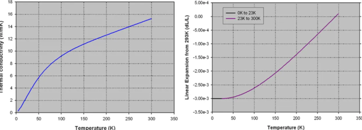
Figure 4.1 – Variation of the thermal conductivity and linear expansion of the aluminium ... 13
Figure 4.2 – Thermal conductivity and linear expansion of the 304 stainless steel. ... 14
Figure 4.3 – Thermal conductivity of Isoval Epoxy. ... 15
Figure 5.1 - Simplified scheme of the thermal system for lumped network analysis ... 16
Figure 5.2 – Electrical transmission line equivalent circuit diagram for modelling heat conduction properties; the physical variables are specified in their thermal equivalents. ... 17
Figure 5.3 – Typical curve of the cooldown. ... 18
Figure 5.4 – CAD model used to simulate the applied thermal loads. On the base-plate, the thermal loads applied for this simulation are -150 and 150 °C. ... 19
Figure 5.5 – Representation of the mesh used in this simulation. ... 20
Figure 5.6 – Thermal analysis to outer epoxy support when large clutch is at -150°C. ... 21
Figure 5.7 – Thermal analysis to outer epoxy support when large clutch is at -150°C. ... 22
Figure 5.8 –a) CAD model used in inner epoxy simulation; b) Representation of the mesh used in this simulation. ... 22
Figure 5.9 – Thermal analysis to inner epoxy support. ... 23
Figure 5.10 – Section view of the CAD model ... 24
Figure 5.11 – Cool down time simulation. ... 24
Figure 5.12 – Cool down fit ... 25
Figure 5.13 – Mechanical switch expansion ... 26
Figure 6.1 – Epoxy after the CNC milling process. ... 27
Figure 6.2 – Display of most parts produced using the CNC machine at the workshop. ... 28
Figure 6.3 – Assembly of the outer epoxy, showing the details of the Mechanical Thermal Switch (flexible bellow and inner epoxy) ... 29
Figure 6.4 – System without the aluminium base-plate. showing the copper thermal interface of the pistons. Inside the red circles it can be seen the position of the temperature sensors. ... 29
Figure 6.5 – The top picture shows the system assembled. On the bottom, a MLI blanks was placed around the outer epoxy as a thermal radiation shield. ... 30
Figure 7.1 – LabJack pinout schematic. ... 31
Figure 7.2 – Omega patch heater attached to the thermal fixation before installation. ... 32
Figure 7.3 – Location of the heat patches on the back plate ... 32
Figure 7.4 – Compact cylinder and solenoid operation description. ... 33
Figure 7.5 – Schematic of the Control Board. ... 34
Figure 7.6 – PCB after the milling and after depositing a very thin layer of tin. ... 34
Figure 7.7 – Board Control final result. All components soldered and operational. ... 35
Figure 7.8 –OMEGA CN7800 front side. ... 35
Figure 7.9 –OMEGA CN7800 read temperature LabVIEW block diagram. ... 36
Figure 7.10 –OMEGA CN7800 checksum calculator LabVIEW block diagram. ... 36
Figure 7.11 – Heat map load of the cold head DE-104(T) from ARS. ... 37
Figure 7.12 – (Left) Water flow sensor exterior (Right) Water flow sensor internal mechanisms .. 38
Figure 7.13 – Warning lights system ... 38
Figure 8.1 – Thermal cycle with temperatures from +150/-150 °C. ... 43
Figure 8.2 – On the left side is the front side of the base plate. in which the samples will be places. as well as the heat resistors. On the right. are shown the pockets on the back side. ... 44
Figure 8.3 – On top. plot temperature gradient on the base plate. On bottom. deformation based on the same temperature gradient as the top plot. ... 45
Figure 8.4 – Section view of the final design for the thermal vacuum cycle sub-system. ... 46
Figure 8.5 – Thermal cycle with temperatures from +150/-150 °C. ... 46
Figure 8.6 – Distribution of the temperature sensor on the MLI sample. ... 47
Figure 8.7 – MLI test samples assembled in the sample holder for thermal characterization of the layers ... 48
Figure 8.8 – Chosen temperature range. from 140 to -120 °C. ... 49
Figure A.1 – Schematic of the sun radiation on a perpendicular surface ... 57
Table of Tables
Table 4.1 – Properties of aluminium 5083 ... 13
Table 4.2 – Properties of stainless steel ... 14
Table 4.3 – Properties of copper ... 14
Table 4.4 – Properties of Epoxy ... 15
Table 5.1 - Corresponding physical variables ... 17
Table 5.2 – Parameters used in the lump model ... 18
Table 5.3 – Mesh description ... 20
Table 5.4 – Mesh description ... 22
Table 5.5 - Parameters determined for the fit of the dynamic simulation result ... 25
Table 7.1 –Warning lights system description ... 38
Table 8.1 – Summary of the time need to complete each cycle with different temperature ranges . 42 Table 8.2 - Summary of the time need to complete each cycle with different temperature ranges 47 Table 8.3 - Summary of the time need to complete each cycle with different temperature ranges 48 Table 8.4 - Summary of the parameters used in the Acceleration Factor calculation. ... 50
Acronyms
AO Atomic Oxygen
AF Accelerated factor
COTS Commercial off-the-shelf EOS Earth Observing Satellite
ESA European Space Agency
GEO Geosynchronous Earth Orbit
HTD High Temperature Dwelling
IC Integrated Circuit
LEO Low Earth Orbit
LTD Low Temperature Dwelling
MEO Medium Earth Orbit
MLI Multi-Layer Insulation PEO polar earth orbit
PSA Pressure-Sensitive Adhesive
RSO Resident Space Object
TVC Thermal Vacuum Cycle
1. Introduction
Optical and radar observations from the ground and the analysis of retrieved hardware, either from maintenance missions on the Hubble Space Telescope or from dedicated missions have shown an abundance of space debris objects, that seem to result from the degradation of outer spacecraft surfaces. Retrieved hardware has shown that Multi-Layer Insulation foils, as well as paint, can severely degrade in space and create a larger number of pieces creating space debris. A quantitative description of the amount and size distribution of these debris objects is lacking.
Every material on the exterior of a spacecraft is exposed to the harsh space environment, which is the cause for degradation of materials. The main threats are the charged particle radiation, ultraviolet radiation, atomic oxygen for low orbits, extreme temperature and thermal cycling, impacts of micrometeoroids and debris. The relative impact of the individual threats depends on the type of mission to be performed, the mission duration, the solar cycles, solar events and the orbit in which the spacecraft will be placed. However, such degradation products could form a considerable part of the debris population and more information is required to develop reliable space debris flux models, compute the impact on risk assessments and for the selection of materials to mitigate these effects.
To better understand the degradation of spacecraft materials, studies can be performed through space-exposures and ground experiments. The opportunity to examine space flown materials, either through recovered material or through dedicated experiments are rare. Differences between the experiment environment and the intended mission environment and synergistic environmental effects requires a cautious interpretation of results. Ground laboratory studies can be used to examine individual environmental effects or a combination of these effects. Laboratory tests can be conducted in a timely manner using accelerated levels for some environmental effects, but due to the difficulties in properly simulate the space effects and complex calibrations, a cautious interpretation of the results is required.
The infrastructure described in this document was developed as part of an ESA project, denominated “Space Debris from Spacecraft Degradation Products”. The main purpose of this activity is the assessment of the amount and characteristics of space debris objects resulting from spacecraft surface degradation. The results are to be used as input for future space debris population models and for the selection of materials in the context of debris mitigation measure.
During the orbit, spacecraft are under space conditions, known for the harshness of several factors. The temperatures on the sunny side of the satellite can rise to nearly +100 °C. On the dark side, the temperature drops below -100 °C. The thermal cycling and the vacuum conditions may have a relevant impact on the lifetime of the spacecraft, which can be in orbit for a period comprised between two and up to ten years. A space environment simulator enables the measurement of the amount of debris resulted from space exposer.
The work here described is part of a system capable of expose, in synergy, Vacuum Ultra Violet and thermal cycling under vacuum. In this document are described all development stages of the thermal vacuum subsystem.
Special attention was given to the thermal isolation of the system, since it operates with a range of 260 °C and a bottommost at -120 °C. Operating at low temperatures involves a careful analysis of the materials to have minimal losses of power.
The cryogenic architecture uses a helium cryocooler as a heat pump and a mechanism that allows the cold part to be engaged and released from the base-plate, denominated Mechanical Thermal Switch. In order to evaluate the cooldown period to be achieved using this architecture, a dynamic simulation was performed.
In order to implement the control system needed to achieve a thermal cycling, a control software based on LabView was developed. Besides providing the user with a graphical interface, it gathers information from several sensors and executes the thermal cycling according to those readings.
As a result, it was possible to achieve several system performance levels. Furthermore, a modification of the original base-plate was required with the intent of decreasing the cooldown time to values within the target time range. Although, the characterization of the Multi-Layer Insulations is addressed in the report, it is not intended to be analysed in detail but to demonstrate the thermal analyses of the system.
2. Motivation and space environment
This chapter intends to provide a contextualization on the system present later in the document. A description of space environments that have impact in spacecraft exterior is presented.
The main goal of the ESA project is to assess the characteristics and the amount of space debris objects created during the exposure of a spacecraft exterior to its operational environment. The emphasis is on Multi-Layer Insulation (MLI) and paint flakes, which are both known as surface degradation products. It is important to understand the generation processes to be able to account for those space debris sources in environmental modelling. Therefore, experimental degradation studies shall be performed under realistic, or accelerated, space environment conditions.
The results of this study will also be used to improve the MASTER (Meteoroid and Space Debris Terrestrial Environment Reference), the European reference model for the space debris environment. The current release is MASTER-2009, which is soon to be replaced by an upgraded version with updated population files. [1]
2.1. Relevant Space Environment
Every material on the exterior of a spacecraft is exposed to the harsh environment of space, which is the cause for the degradation of materials. The main threats are charged particle radiation, ultraviolet radiation, atomic oxygen, extreme temperature and thermal cycling, impacts of micrometeoroids and debris. The relative impact of the individual threats depends on the type of mission to be performed, the mission duration, the solar cycles, solar events and the orbit in which the spacecraft will be placed at.
2.1.1. Orbit Definition
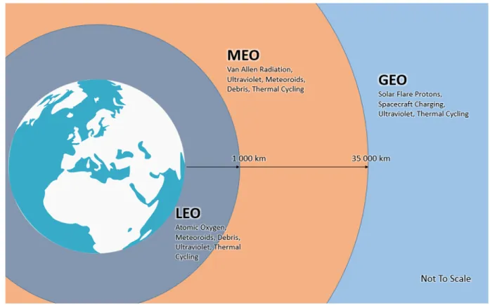
The relative impact of any of the space environment effects on materials depends on the type of mission the spacecraft must perform, e.g. communication, defence, Earth observation, and more important, the orbit in which the spacecraft is placed. Figure 2.1 shows the main factors of satellite surface degradation in the space environment as a function of orbit altitude. To establish the scale, please take in mind that the Earth radius is around 6370 km.
Figure 2.1 - Earth orbital definition • Low Earth Orbit
LEO refers to orbits in the 100 to 1000km altitude range, which includes Earth-observing satellites (EOS). A particular case to be noted is the International Space Station (ISS) at about 400km. The radiation environment in LEO is rather benign, with a typical dose rate of around 0.1 krad/year. For a mission with a typical duration of 3 to 5 years the total dose is less than 0.5 krad. Most PEO (Polar Earth Orbit) are LEO with high inclinations (>55°) although more eccentric. The high inclination takes the orbit through the polar aurora regions, which can be rich in ion cosmic ray and solar flare particles. Higher radiation dose is accumulated during the passage through these regions; nevertheless, the transition time is typically small in comparison to a full orbit time. Thus, the dose rate is a few krad/year, similar to that in LEO.
A vehicle in LEO will receive radiant thermal energy from three primary sources: the incoming solar radiation (described by the solar constant), reflected solar energy (Earth albedo energy), and outgoing longwave radiation emitted by the Earth and atmosphere. The temperature range goes from -100°C to 100°C. A spacecraft in LEO moves in and out of eclipse once every orbit, as often as every 90 minutes.
• Medium Earth Orbit
The radiation environment in MEO - 1000 km to 35000 km altitude - is harsh since the satellite trajectories are confined, mostly, within the Van Allen radiation belts. Satellites are usually positioned in regions somewhat lower though, variable particle density may occur between the belts. The dose rate from both protons and electrons can be in the order of 100krad/year and it is highly variable due to strong solar cycle effects. Because of that MEO is only used if no other alternatives exist, e.g. GPS,
• Geosynchronous Earth Orbit
GEO is located at 35000km altitude in the high-energy plasma sheet. GEO satellites are exposed to the outer radiation belts, solar flares and cosmic rays [2,3].
2.1.2. Temperature
Temperature is a major parameter in the process of materials degradation when acting in synergy with other components of space environment, especially radiation. Regarding organic materials degradation increases with temperature due to the greater chain mobility (higher scission/x-linking ratio) [3]. In inorganic materials temperature governs annealing of coloured centres as observed in optics [4]. At low temperature, synergy with space radiation is not straightforward and depends on materials type: degradation mechanisms are “frozen” in materials sensitive at room temperature, while no significant change is observed in more resistant materials (epoxy, polyimide), silicones are more sensitive at low temperatures.
For missions with demanding temperature constraints (range and cycling), it was shown that the representative simulation of the mission profile was required to expect a reliable estimate materials degradation and prediction of End-of-Life performances [5].
A simple calculation allows to estimate the temperature of a surface facing the sun, with a 90° angle, of 115 °C. (Appendix A).
Moreover, at macroscopic level, temperature cycling alone or in synergy with space radiation induces mechanical stress that can result in enhanced overall degradation or at stress location [6,7].
2.1.3. Vacuum
The hard vacuum of space (10-6 to 10-9 mbar) will cause outgassing, which is the release of volatiles
from materials. The outgassed molecules then deposit on line-of-sight surfaces and are more likely to deposit themselves on cold surfaces.
2.1.4. AO
Several forms (allotropes) of oxygen exist, while O2 (molecular oxygen) being the most familiar
since represents the breathable form on Earth. Ozone (O3) and atomic oxygen (O1, single atom,
abbreviated AO), both occur in the upper atmosphere and pose distinct reactive allotropes. The atomic oxygen is very chemically active and it is the major atmospheric component in the low earth orbit [8,9]. The AO erodes most organic materials will react with many metals and other inorganic materials. The Atomic Oxygen only occurs on LEO.
2.1.5. VUV
Earth’s atmosphere filters out most of the sun’s damaging light, but outside this protection exterior spaceship materials bear the brunt of solar photon damage. The Vacuum UV (VUV) is the most damaging UV band in terms of material degradation and its wavelength is between 100 and 200 nm.
2.2. Materials and debris generations
A typical spacecraft has a payload, where the equipment for the primary mission is located and a bus or platform where the subsystems are installed. These subsystems typically include the Structures
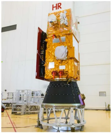
subsystem, the Electrical power/distribution subsystem, the Telemetry, tracking, and command subsystem, the Attitude/velocity control subsystem, the Propulsion subsystem and the Thermal-control subsystem. On the Structures subsystem is assembled (among others) the external structure of the spacecraft [10,11]. The spacecraft external surface is mostly composed of either insulation blanket or radiator surface materials. Both are classified under the thermal control subsystem. As seen, for example, in Figure 2.2 or in any typical picture of a satellite, its surface looks golden in colour. The golden colour comes from the outer layer of the MultiLayer Insulation (MLI) blankets. The spacecraft exterior is mostly blanketed with MLI with cut-outs for radiator surfaces. The remaining radiator surfaces can be, for example, thermal (black body) radiators for temperature control, a second surface mirror or a more rigid blanket or tile attached to the spacecraft structure. It can also be an optical solar reflector or a paint.
Figure 2.2 - Sentinel-2B installed on its payload launcher adapter (courtesy of ESA)
2.2.1. Paint
There is only a basic understanding of the processes leading to the generation of paint flakes as surface degradation particles. The driving factors can be confined to atomic oxygen, thermal cycling and ultraviolet radiation. While paint flakes may also be generated through the impacts of meteoroids and space debris as spallation products.
A spacecraft in LEO to be subject to the influence of Earth’s outer atmosphere, where atomic oxygen reacts with its surface. For many materials like silver, polymers or some metallic surfaces, oxidation processes lead to the creation of a brittle layer, which may crack and lead to the generation of spall off
This mechanism would apply to susceptible substrates only and not to aluminium. The paint flake size distribution of spalls generated during such a process is difficult to model. [12]
Thermal cycling due to large temperature fluctuations during eclipse entry/exit leads to a thermal expansion of coatings and substrates at different rates, creation of cracks caused by thermal stress, growth of cracks caused by thermal stress combined with intrinsic stress, delamination1 between a
cracked coating layer and substrate leading to the shedding of flakes (µm to mm sizes). Moreover, additional UV radiation and exposure to atomic oxygen may accelerate this process. The modelling of these processes is quite complicated as the degradation processes are highly dependent on material properties, while the variety of materials used on different spacecraft and upper stages is large. Even among specific material types, like paints, there is a large diversity of properties. One of the main problems is to define the parameters describing the size distribution and the release rates for paint flakes.
In the model MASTER-2009, for example, a power law is used for the size distribution, based on validation data from returned surfaces from the Space Shuttle and LDEF2 [13]. The release rates are
based on a model published by Maclay and McKnight [14], considering releases due to the above-mentioned factors. The shape of the individual flakes in MASTER-2009 is assumed to be spherical and the density is a mean density of 4700 kg/m³, representing a mean value out of zinc, titanium and aluminium, materials typically used for paint; for the velocity distribution, a release velocity of 1 m/s is assumed for all particles [15].
2.2.2. Multi-Layer Insulation
There are two major sources resulting in the generation of MLI space debris objects: • Thermal protections MLI from satellites/spacecraft;
• Sun-shielding MLI, which were used on radio-frequency antennas.
MLI space debris objects are generated through delamination processes. A range of surface degradations mechanisms drives the delamination process, e.g.:
• Thermal Cycling due to Sun and shade phases; • Irradiation by the extreme ultra violet spectrum;
• Charged particle radiation and solar flare x-ray exposure; • Atomic oxygen effects in low Earth orbits.
The ductility of the MLI material is a crucial point in the delamination process: embrittlement3
through exposure to radiation or atomic oxygen promotes crack propagation through the material. However, atomic oxygen has also been found to increase the material ductility [16]. This occurs when carbon-carbon bonds near the surface have been severed through solar irradiation or reaction with atomic oxygen, which increases the susceptibility to foil tearing. The ’loosened’ carbon chains can then be removed by, again, reacting with atomic oxygen, smoothing over the surface. Typical materials used for MLI are: Kapton®, Mylar®, Teflon® FEP and Tedlar® PVF with, typically, vapour deposited aluminium. [17]
A key aspect of MLI space debris fragment modelling is the parametrization of the area to mass ratio (A/m) of the generated fragments. The ratio depends on used materials and layer thickness. In a MLI
1 Delamination is a mode of failure for composite materials and metals, that can occur with repeated cyclic
stresses (thermal and mechanical), from oxidized metals and impacts and can cause layers to separate with significant loss of mechanical toughness.
2 Long Duration Exposure Facility was an experiment to provide the effects of long-term exposer of materials
to space environment.
stack for thermal protection, the outer and inner layers are thicker than the reflector layers in between. Common thicknesses are 5 mil for the outer layers and 0.25 mil for the reflector layers (1 mil = 0.001 inch ≈ 25.4 μm). The material densities ranges are from 1.4 g/cm3 to 2.2 g/cm3.
Via a determination of a characteristic length of MLI debris parts it is possible to calculate debris part area and mass. In MASTER.2009 model the area is assumed as the square of the characteristic length. The characteristic length derives from data sets based on results of ground tests that have been performed by Kyushu University (Japan) and NASA [13] Orbital Debris Program Office, even though the available data is limited.
3. System Concept
3.1. System Requirements
Spacecraft are exposed to continuous temperature changes e.g. due to changing sun irradiation. For materials to be capable for space applications the performance under changing ambient temperatures in vacuum is an important issue. The thermal-cycling test may be used to assess materials for their space capability. The test setup used for thermal cycling of samples consists of a heating/cooling plate.
In order to simulate the space environment, the ESA Standard4 recommends performing 100 cycles
between -100ºC and 100°C under vacuum (10-5 Pa) with a dwell time of 5 minutes minimum and a slope
of 10°C per minute.
3.2. Different approaches
Concerning the fulfilment of the requirements above mentioned several architectures were evaluated. To achieve the high temperature needed an easy solution is the use of heating resistors, they can be purchased for vacuum applications and the output power adjusted as needed.
For the low temperature requirement, the most common and widely used in cryogenic applications for temperatures from -100 to -200 °C is liquid nitrogen, with a reservoir of liquid nitrogen inside the chamber, it is possible to have a cold source at the temperature of the nitrogen’s vaporization, 78 Kelvin. When speaking of applications where the temperatures are maintained constant this approach works very well, however, in cycles with a high range like the one described in the requirements, the nitrogen consumption is too high, as well as the price and there is also the question of a large enough Dewar to keep the demand.
Another solution could be based on the Peltier effect (thermoelectric cooling). It is the phenomenon that a potential difference applied across a thermocouple causes a temperature difference between the junctions of the different materials in the thermocouple. For low temperature, a commercial Peltier cell is not available and the efficiency is well below 10% [18].
An additional solution, is the Vapor-Compression Refrigeration, it is because it is easy to build a low-cost cooling device employing this method. Air conditioners in car and at home uses a vapor-compression cycle to cool the ambient air temperature. The vapor-vapor-compression refrigeration cycle is comprised of four steps: compression, condensation, throttling and evaporation. The drawback with a vapor-compression is that for the low temperatures, below -60 °C, the fluids based on Ammonia are not suitable, so an alternative fluid would be necessary. [19]
The helium based compressor/expansion cryocooler systems are normally used to achieve lower temperatures. These systems are mainly developed to cool down small material samples to enable physical studies. The heat power is however limited and we were fortunate to have already in the group a rather powerful helium compressor/expander system.
The thermal switching between the heating and cooling stages is also a challenge. One interesting technology is to use thermal switches where a small, but large area, material gap achieves variable thermal conduction by varying the pressure of a thermal conducting gas. The pressure is usually varied, inside the cryostat by including an adsorption pump in the gas reservoir. The heat flow in these systems is however highly limited [20]
A mechanical switch between hot and cold masses had to be implemented inside the cryostat system and typically would require the usage of cryogenic motors or, at least, cryogenic mechanisms or magnetic coils to exert appreciable contact forces between the temperature coupling parts.
Another option was to use an external mechanical system that would directly exert the mechanical contact forces tough a mechanical connection inside a vacuum bellow. Thermal isolation and careful vacuum wall design are still a challenge.
Those were the first ideas about this subject while presenting their advantages and weak points. In the next section, the chosen architecture is presented and explained in detail.
3.3. Design Description
Figure 3.1 – Thermal Vacuum Cycle Conceptual Design
The chosen architecture is based on the use of a Helium cryocooler as a cold source and the resistors as heaters. From the conceptional point of view, the cold source must have a thermal interface that disengages when the heaters are working, preventing unnecessary heat flowing to the cryocooler. This concept architecture allows the operation to work unattended for extended periods.
The Figure 3.1 shows the conceptual design of the TVC system. In particular, the Thermal Mechanic Switches which implements the thermal interface between the cold finger and the base-plate.
The thermal cycling will be performed on a vacuum chamber with 10-5 mbar of pressure and a
temperature range from -150 to 150°C. This higher temperature range is used in order to create accelerated test conditions over the operation conditions. Usually, the term acceleration factor (AF) is used to refer the ratio of the acceleration characteristic between the operation level and a higher test level. A calculation of the AF is provided in chapter 8.4, as part as the performance of the system.
The main vacuum chamber had already been developed in the group [21] and was available for these studies. The overall dimensions are of a 1m long cylinder that has an inner dimeter of about 60cm.
The sample holder (where the MLI and the paints are to be assembled) will be assembled on top of an aluminium base plate5 that will be heated/cooled. During cool down, the cold finger will be put in
contact with the baseplate by means of mechanical thermal switches.
The thermal switching, i.e. hot to cold and vice-versa, is achieved with the use of three pneumatic pistons connected to the cold source. When disconnected, the heaters are turned on to reach the top temperature and to perform a cooldown, the heaters are turned off and the pneumatics are engaged. The thermal connection between the cold finger and the pistons is made with copper straps.
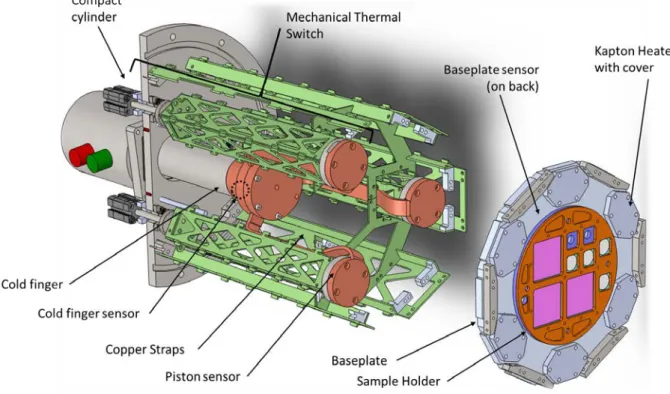
Figure 3.2 – Detail model of the chosen design Below there is a description of the items presented in Figure 3.2:
• Mechanical Thermal Switch
The mechanical switches consist in compressed air pneumatic system using a flexible bellow as a linear vacuum feedthrough. The cold part is isolated by an epoxy with low thermal conductivity, used in cryogenics and vacuum applications. This system allows to disconnect the cold source from the hot source mechanically.
• Baseplate
The baseplate is the part of the system where the resistors are attached, and the thermal connection with the cold finger is made on its back. And where the samples to be tested will be placed.
• Heater
For heater, we selected Kapton flexible foils [22] because they have a wide operational temperature and we have used them in the past for this kind of application. The Kapton foil heaters will be positioned between the sample holder and the baseplate.
• Heat Pump
A helium cryocooler is used to cool down the baseplate. The cryocooler [23], at -150 ℃, is able to remove 90 watt. The section area of the copper strip can be customized to fit the desired power flux.
• Thermal Isolation
Besides the isolations provided by the epoxies, a MLI blanket is used to shield from the radiation emitted by the chamber walls, at room temperature.
In order to fulfil the ESA standard requirements there will be 4 stages: Warm Up, High Temperature Dwelling (HTD), Cool Down and Low Temperature Dwelling (LTD). The temperature control will be achieved by:
a) Monitoring the sample holder with PT100 temperature sensors, due to low voltage measurements, Omega controllers [24]will be used;
b) Heating procedure:
i. During heating, the thermal switch will disconnect thermally the cold finger from the back plate;
ii. The Kapton resistors will be tuned on up to achievement of the top temperature (e.g. 150 °C);
c) During cool down:
i. The resistors will be turned off and the mechanical thermal switches will be turned on, connecting thermally the cold finger to the back plate. This situation will endure up to minimum temperatures (e.g. -150 °C);
4. Material selection
Materials for the different parts of the system were selected based on part function and their mechanical/thermal proprieties. Previous experiences with some materials, in terms of machining and procurement, were fundamental during the process of selection.
The thermal conductivity of a material, gives its ability to transfer the heat. In a material with a high thermal conductivity will have a heat flux higher than a material with a low thermal conductivity.
•
Aluminium
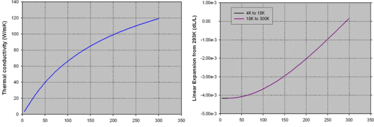
The 5083 aluminium is known for exceptional performance in extreme environments. The 5083 aluminium is a lightweight, strain hardened, corrosion resistant and high strength alloy is commonly used in high strain rate applications such as those experienced under shock loading [25].
Table 4.1 – Properties of aluminium 5083, at 25 °C
Physical Property
Value
Density 2660 kg/m³
Tensile Strength 290 MPa
Elastic Modulus 70 GPa
Thermal Expansion 24 x10-6 /K
Thermal Conductivity 121 W/m.K
Specific Heat 900 kJ/kg.K
Figure 4.1 – Variation of the thermal conductivity and linear expansion of the aluminium 6
•
Stainless Steel
Austenitic stainless steels are the most common choice for high vacuum and ultra-high vacuum systems. The 304 stainless steel is a common choice of a stainless steel.
Table 4.2 – Properties of stainless steel, at 25 °C
Physical Property
Value
Density 8000 kg/m³
Tensile Strength 517 MPa
Elastic Modulus 190 GPa
Thermal Expansion 18 x10-6 /K
Thermal Conductivity 16 W/m.K
Specific Heat 500 kJ/kg.K
Figure 4.2 – Thermal conductivity and linear expansion of the 304 stainless steel.
•
Copper
Oxygen-free high thermal conductivity (OFHC) copper is widely used in cryogenics. Due to its high purity, 99.99%, it is expensive. The copper is a good heat exchanger due to its good thermal conductivity. The copper is used in the thermal straps and where they attached, namely, the cold finger and the pistons.
Table 4.3 – Properties of copper, at 25 °C
Physical Property
Value
Density 8900 kg/m³
Tensile Strength 395 MPa
Elastic Modulus 110 GPa
•
Epoxy
The ISOVAL® FR4-HF is a halogen free epoxy glass laminate with a limiting temperature of 180
°C. Epoxy glass laminates are even usable for cryogenic applications at temperatures close to absolute zero. Also for these laminates an increase in mechanical strength and modulus of elasticity can be observed but also at very low temperature for example, in liquid nitrogen or liquid helium they do not show vitreous embrittlement as rubber or thermoplastics do.
Table 4.4 – Properties of Epoxy, at 25 °C
Figure 4.3 – Thermal conductivity of Isoval Epoxy.
7 A thermal expansion is not available from the manufacture datasheet. A conservative value was used.
Physical Property
Value
Density 2000 kg/m³
Tensile Strength 374 MPa
Elastic Modulus 18.9 GPa
Thermal Expansion7 30 x10-6 /K
5. Thermal Simulations
In this case, as in any other engineering problem, the analysis of mechanical systems has been addressed by deriving differential equations relating the variables of through basic physical principles such as, conservation of energy and the laws of thermodynamics. However, once formulated, solving the resulting mathematical models is often impossible, especially when the resulting models are nonlinear partial differential equations. In this chapter, the thermal analysis of the chosen architecture, using both analytical lumped circuit and numerical finite element methods are presented.
5.1. Approximated Lumped Network Analysis
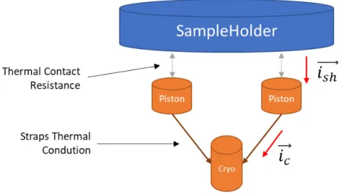
In Figure 5.1 a simplified scheme of the thermal system is shown. As a rough approximation, the thermal contact resistance between the Sample Holder and the Pistons is considered insignificant, however the heat flux is limited by the area and length of the copper part of the piston. The thermal straps also add a resistance to the heat flux.
As a convention, the heat flows from the Sample Holder (at a higher temperature) to the Cryocooler (at a lower temperature).
Figure 5.1 - Simplified scheme of the thermal system for lumped network analysis
An effective way to better understand the thermal problem is to use the analogy between thermal and electrical networks. The voltage (rather than temperature) at various nodes can be calculated together with the current (rather than heat) flow between nodes. For transient analysis, electrical capacitances (rather than thermal capacitances) are added to account the change internal energy of the body with time. The thermal resistances are resultant from geometric dimensions, thermal properties of the materials and heat transfer coefficients. [26,27]
The equivalent circuit diagram that relates the heat path from the Sampler Holder to the Cryocooler is depicted in Figure 5.2. Where the generator, 𝑉𝑉𝑐𝑐, is the temperature in the cryocooler, 𝑅𝑅𝑇𝑇 is the sum of the internal resistance of the cryocooler and the thermal conduction of the copper straps, 𝐶𝐶𝑝𝑝 is the heat capacity of the pistons, 𝑅𝑅𝑐𝑐 is the contact resistance between the pistons and the sample holder and 𝐶𝐶 is the heat capacity of the sample holder.
Figure 5.2 – Electrical transmission line equivalent circuit diagram for modelling heat conduction properties; the physical variables are specified in their thermal equivalents.
Table 5.1 - Corresponding physical variables
Thermal Electrical
Temperature K Voltage V
Heat flow W Current A
Thermal resistance K/W Resistance V/A
Thermal capacitance Ws/K Capacitance As/V
For the circuit in Figure 5.2, the following equation system that describes it is retrieved.
⎩ ⎪ ⎪ ⎪ ⎨ ⎪ ⎪ ⎪ ⎧ 𝑖𝑖𝑠𝑠ℎ= −𝐶𝐶𝑠𝑠ℎ𝑑𝑑𝑉𝑉𝑑𝑑𝑑𝑑𝑠𝑠ℎ 𝑉𝑉𝑠𝑠ℎ− 𝑉𝑉𝑝𝑝= 𝑅𝑅𝑐𝑐𝑖𝑖𝑠𝑠ℎ 𝑖𝑖𝑠𝑠ℎ− 𝑖𝑖𝑐𝑐= 𝐶𝐶𝑝𝑝𝑑𝑑𝑉𝑉𝑑𝑑𝑑𝑑𝑝𝑝 𝑉𝑉𝑝𝑝− 𝑉𝑉𝑐𝑐= 𝑅𝑅𝑇𝑇𝑖𝑖𝑐𝑐 𝑖𝑖𝑐𝑐 = 𝑘𝑘0𝑉𝑉𝑐𝑐+ 𝑘𝑘1 (1) (2) (3) (4) (5)
Particular solutions are in the form of:
𝑋𝑋⃗ = 𝐶𝐶����⃗𝑎𝑎𝑒𝑒0 −𝑎𝑎𝑎𝑎 (6) ⎣ ⎢ ⎢ ⎢ ⎢ ⎢ ⎡ 0 0 𝐶𝐶𝑠𝑠ℎ𝑎𝑎 1 0 0 −1 1 −𝑅𝑅𝑐𝑐 0 0 −𝐶𝐶𝑝𝑝𝑎𝑎 0 1 −1 −1 1 0 0 −𝑅𝑅𝑇𝑇 −𝑘𝑘0 0 0 0 1 ⎦ ⎥ ⎥ ⎥ ⎥ ⎥ ⎤ ⎣ ⎢ ⎢ ⎢ ⎢ ⎡ 𝑉𝑉𝑐𝑐0 𝑉𝑉𝑝𝑝0 𝑉𝑉𝑠𝑠ℎ0 𝑖𝑖𝑠𝑠ℎ0 𝑖𝑖𝑐𝑐0 ⎦ ⎥ ⎥ ⎥ ⎥ ⎤ = ⎣ ⎢ ⎢ ⎢ ⎢ ⎢ ⎡0 0 0 0 𝑘𝑘1⎦ ⎥ ⎥ ⎥ ⎥ ⎥ ⎤ (7)
There are two solutions for 𝑎𝑎 are given by:
The constants 𝑅𝑅𝑇𝑇 and 𝑅𝑅𝑐𝑐 were calculated as the inverse of the thermal conductivity. For 𝑅𝑅𝑇𝑇 was used the length of the copper straps and it section. The lack of studies about surface-to-surface contact in vacuum, between aluminium and copper, 𝑅𝑅𝑐𝑐 was assumed to be limited by the thermal conductivity of the copper part of the pistons. 𝐶𝐶𝑠𝑠ℎ was determined by the heat capacity of the sample holder, made entirely of aluminium. 𝐶𝐶𝑝𝑝 was calculated by adding the heat capacity of the stainless steel and copper of the piston. Table 5.2 shows the determined constants.
Table 5.2 – Parameters used in the lump model
Parameters Value
𝐶𝐶𝑝𝑝 832.5
𝐶𝐶𝑠𝑠ℎ 291.35
𝑅𝑅𝑇𝑇 4.867
𝑅𝑅𝑐𝑐 6.64E-03
Replacing equation (8) with the constants in the previous table two solutions for a are obtained. The solutions are:𝑎𝑎 → {6.979 × 10−01, 1.396 × 10−04} ,meaning the solution is a linear combination of two exponential. This result was expected since there are two mechanisms involved in the cooling process, one from the thermal mass of the pistons, a very quick process, and a second form the conduction on the straps. The typical curve of this cooldown is shown on Figure 5.3
Figure 5.3 – Typical curve of the cooldown.
𝑎𝑎 = 𝑘𝑘𝑜𝑜�𝐶𝐶𝑝𝑝𝑅𝑅𝑇𝑇+𝐶𝐶𝑠𝑠ℎ(𝑅𝑅𝑐𝑐+𝑅𝑅𝑇𝑇)�+𝐶𝐶𝑠𝑠ℎ+𝐶𝐶𝑝𝑝
2𝐶𝐶𝑝𝑝𝐶𝐶𝑠𝑠ℎ𝑅𝑅𝑐𝑐(𝑘𝑘𝑜𝑜𝑅𝑅𝑇𝑇+1) ±
��𝑘𝑘𝑜𝑜�𝐶𝐶𝑝𝑝𝑅𝑅𝑇𝑇+𝐶𝐶𝑠𝑠ℎ(𝑅𝑅𝑐𝑐+𝑅𝑅𝑇𝑇)�+𝐶𝐶𝑠𝑠ℎ+𝐶𝐶𝑝𝑝�2−4𝑘𝑘𝑜𝑜𝐶𝐶𝑝𝑝𝐶𝐶𝑠𝑠ℎ𝑅𝑅𝑐𝑐(𝑘𝑘𝑜𝑜𝑅𝑅𝑇𝑇+1)
2𝐶𝐶𝑝𝑝𝐶𝐶𝑠𝑠ℎ𝑅𝑅𝑐𝑐(𝑘𝑘𝑜𝑜𝑅𝑅𝑇𝑇+1)
5.2. Finite Element Method
The finite element method (FEM) is the dominant discretization technique in structural mechanics. The basic concept in the physical interpretation of the FEM is the subdivision of the mathematical model into disjoint (non-overlapping) components of simple geometry called finite elements or elements for short. The response of each element is expressed in terms of a finite number of degrees of freedom characterized as the value of an unknown function, or functions, at a set of nodal points.
The response of the mathematical model is then considered to be approximated by that of the discrete model obtained by connecting or assembling the collection of all elements. All analyses were performed using the Simulation Add-in in SolidWorks.
For the TVC system the main concern was the thermal conductivity, either from the hot base-plate to the flange, dissipating needed power to raise the base-plate temperatures or from the flange to the cold base-plate. These simulations are referred as Static Analyses.
A dynamic Simulation was also accomplished in order to assess the time needed for a full cooldown of the system, from 150 to -150 °C.
5.2.1. Static Analyses
A static simulation was performed on the fiberglass epoxies, both inner and outer, in order to determine the quantity of heat transfer during a thermal cycle. To assess those quantities, the extreme temperatures were considered as a worst-case scenario.
• Outer Epoxy
The outer epoxy experiences both high and low temperatures at one end and the other is attached to the flange, which gives a good thermal connection, so it stays always at room temperature.
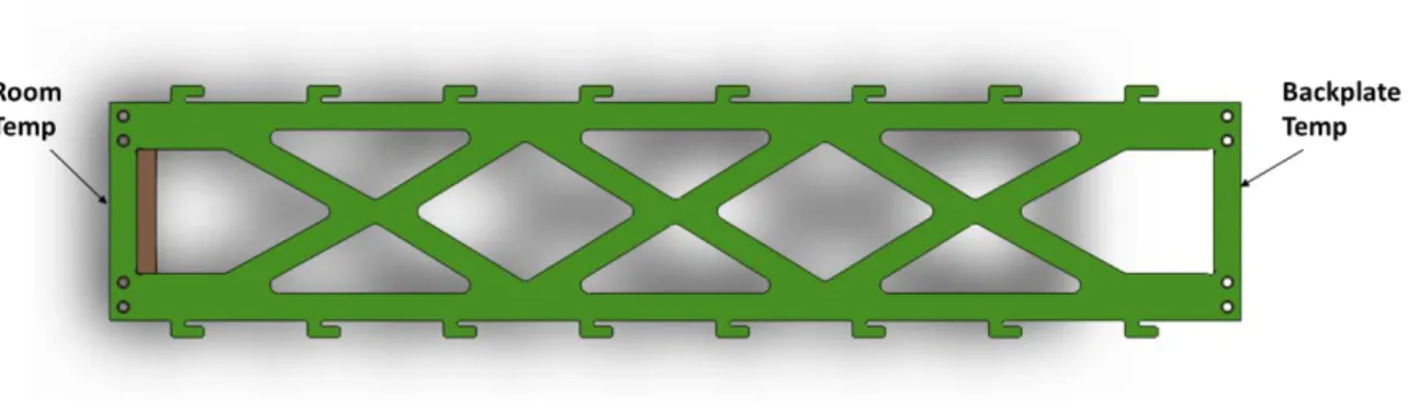
Figure 5.4 – CAD model used to simulate the applied thermal loads. On the base-plate, the thermal loads applied for this simulation are -150 and 150 °C.
A mesh is a discretization of the CAD model. Finite elements and nodes define the basic geometry of the physical structure being modelled, splitting the geometry into relatively small and simple geometric entities, called finite elements. The use of the term “finite” is to emphasize the fact that those elements infinitesimally small, but only reasonably small in comparison to the overall model size.
Each element in the model represents a discrete portion of the physical structure, which is, represented by many interconnected elements. Shared nodes connect these elements to one another.
The greater the mesh density (that is, the greater the number of elements in the mesh), the more accurate the results will be. As the mesh density increases, the analysis results converge to a unique
solution, increasing the computer time required for the analysis. The solution obtained from the numerical model is generally an approximation to the solution of the physical problem being simulated.
A good quality mesh is important for obtaining accurate results from simulations, having different quality check criteria to measure the quality of the mesh. An important parameter in the assessment of the mesh quality is the Aspect Ratio Checks. [28] The simulation accuracy is best achieved by a mesh with uniform size elements whose edges are equal in length. So, by definition, the aspect ratio of a perfect tetrahedral is 1.0.
The Table 5.3 summarizes the mesh used in this simulation. Since 89% of the elements have an aspect ratio below 3.0, the mesh is considered of good quality. Figure 5.5 shows the mesh obtained.
Table 5.3 – Mesh description Mesh information
Mesh type Standard mesh
Total Nodes 36158
Total Elements 18379
% of elements with Aspect Ratio < 3 89 %
% of elements with Aspect Ratio > 10 0.0326 %
Figure 5.5 – Representation of the mesh used in this simulation.
In these simulations only thermal conductivity was considered, a good approximation since in vacuum there is no convection and assuming that all thermal radiation from the wall of the chamber, at room temperature, are shielded by the MLI blankets.
These simulations are driven by the following heat balance equation
𝑄𝑄 −𝜕𝜕𝑞𝑞𝜕𝜕𝜕𝜕 −𝑥𝑥 𝜕𝜕𝑞𝑞𝜕𝜕𝜕𝜕 −𝑦𝑦 𝜕𝜕𝑞𝑞𝜕𝜕𝜕𝜕 = 𝑐𝑐𝑐𝑐𝑧𝑧 𝜕𝜕𝜕𝜕𝜕𝜕𝑑𝑑 (9) where 𝑞𝑞𝑥𝑥, 𝑞𝑞𝑦𝑦 and 𝑞𝑞𝑧𝑧 are the heat flux in the 𝜕𝜕, 𝜕𝜕 and 𝜕𝜕 directions, 𝑄𝑄 is the internal heat generated/absorbed by the body (volume), 𝑐𝑐 is specific heat, 𝑐𝑐 is mass density and 𝜕𝜕 is temperature.
The Fourier's law of heat conduction relates heat flux and temperature and is proportionality constant to 𝑘𝑘, the thermal conductivity. For an orthotropic body (volume element), with the axes of orthotropy coinciding with the coordinate axes the Fourier heat conduction equation is
Joining (9) and (10)
𝑄𝑄 = 𝑐𝑐𝑐𝑐𝜕𝜕𝜕𝜕𝜕𝜕𝑑𝑑 − 𝑘𝑘∇��⃗2𝜕𝜕 (11)
The analysis of steady-state heat conduction problems involves setting the term 𝜕𝜕𝜕𝜕 𝜕𝜕𝑑𝑑� equal to zero and with 𝑄𝑄 assumed to be independent of time.
Taking this into account, in the first simulation the baseplate is considered at 150 °C. As described in Figure 5.4, the temperature applied on the left side is the flange temperature, at room temperature, so 25 °C, and on the right the 150 °C is applied.
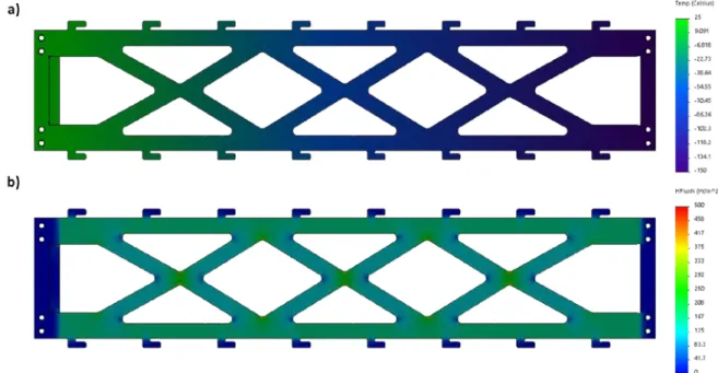
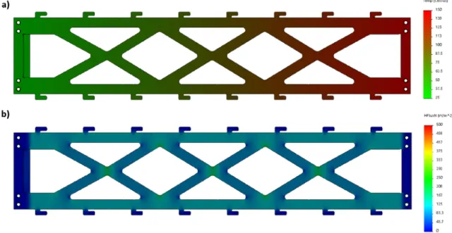
In Figure 5.6, there are plotted the results of this simulation. The top plot shows the temperature gradient on the epoxy and on the bottom the heat flux. The important result here is the total power transferred throw the epoxy, which should be the minimum. The simulation shows 0.02 watts being transferred.
Figure 5.6 – Thermal analysis to outer epoxy support when large clutch is at -150°C.
In a) is plotted a temperature map and in b) the heat flux. The power transferred in this simulation was about 0.02 watt.
Since the model is the same, it was used the same mesh to simulate it with a different temperature in the extremity, the result is as plotted below. Again, the top plot of Figure 5.7, shows the temperature gradient on the epoxy and on the bottom the heat flux. The power transferred was 0.015 watt.
Figure 5.7 – Thermal analysis to outer epoxy support when large clutch is at -150°C.
In a) is plotted a temperature map and in b) the heat flux. The power transferred in this simulation was about 0.015 watt.
• Inner Epoxy
The inner epoxy is connected at one end to the flexible bellows, so one can assume it at room temperature, while the other end is attached to the copper strips. The temperature of the strips for the purpose of this simulation is considered to be at -150 °C, at all times.
Figure 5.8 –a) CAD model used in inner epoxy simulation; b) Representation of the mesh used in this simulation.
By analysing the Table 5.4, one can conclude that the mesh is good since 91% of the elements have an aspect ratio smaller than 3.
Mesh information
Mesh type Standard mesh
Total Nodes 45214
Total Elements 25606
% of elements with Aspect Ratio < 3 91.5 %
% of elements with Aspect Ratio > 10 0.133 %
In Figure 5.9, the results of the simulation are plotted. The top plot shows the temperature gradient on the epoxy and on the bottom the heat flux. The important result here is the total power transferred throw the epoxy, which should be the minimum. The simulations show that 0.02 watts are transferred.
Figure 5.9 – Thermal analysis to inner epoxy support.
5.2.2. Dynamic Simulation
The dynamic simulations were performed in order to assess the time needed for a cooldown. A simplified CAD model was used for this simulation. It is shown in Figure 5.10, the CAD model used for this simulation. The output power of the cryocooler is depended of its temperature and that dependency was used in the simulation and the base plate was set to 150 °C, as initial temperature.
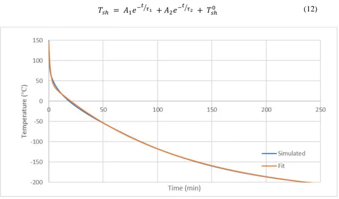
The results of this dynamic simulation are shown in the plot Figure 5.11.
Figure 5.10 – Section view of the CAD model
Figure 5.11 – Cool down time simulation.
In order to compare this result with the one obtained from the lumped model in 5.1, it is necessary to perform a non-linear fitting on the temperature of the sample holder. A two-phase exponential decay function with time constant parameters model was used. The equation for the two-phase exponential decay function is:
𝜕𝜕𝑠𝑠ℎ = 𝐴𝐴1𝑒𝑒−𝑎𝑎 𝜏𝜏�1 + 𝐴𝐴2𝑒𝑒−𝑎𝑎 𝜏𝜏�2 + 𝜕𝜕𝑠𝑠ℎ0 (12)
Figure 5.12 – Cool down fit
For the fit of the temperature on the sample holder over time, it is possible to determine the two-time constant parameters, 𝑎𝑎1 and 𝑎𝑎2. The following table shows the parameters calculated:
Table 5.5 - Parameters determined for the fit of the dynamic simulation result
Variable Value Standard Error
𝜕𝜕𝑠𝑠ℎ0 -236.735 0.693
𝐴𝐴1 99.960 1.576
𝜏𝜏1 93.728 2.992
𝐴𝐴2 281.677 0.541
𝜏𝜏2 6974.883 44.291
Inverting 𝜏𝜏 parameters to get the 𝑎𝑎1 and 𝑎𝑎2 to compare with the ones in section 5.1, it became: 𝑎𝑎⃗ → {1.067 × 10−02. 1.434 × 10−04}
For the first exponential, the one with higher decrease in velocity, it represents a difference of a decrease of 98% over the initial estimated in lumped model. This means that the thermal contact between the Base Plate and piston was over estimated in the lumped model, making this process slower. The second exponential term was increased by 3%.
5.3. Thermal Expansion
This is only a brief discussion about thermal expansion since it does not play a major role in this system. Even with the temperature ranges expected for this system, the expansion is in the order of a few micrometres. For instance, the expanse of the stainless steel in the parallelepiped (see Figure 5.13) is 0.135 mm and in the epoxy, is 0.266 mm (Appendix B) . This means that alignment pins are not an option, but the use of screws is acceptable.
6. System Development
After the validation of the design. the parts needed to be manufactured (in-house or from external companies) and the COTS obtained. In this chapter. the manufacture processes are described. as well. as the assembly process.
6.1. Manufacture
All parts in aluminium and epoxy were produced in the Department of Physics’ workshop with the aid of a 3D milling machine. The parts drawn in SolidWorks were converted in g-code file using SolidCam8. Afterwards. the CNC software interprets the g-code and reproduces the 3D models.
Figure 6.1 – Epoxy after the CNC milling process.
8 SolidCam is a plug-in that is fully associative with the SolidWorks design model, so that is possible to
Figure 6.2 – Display of most parts produced using the CNC machine at the workshop.
The Inox and copper parts were outsourced. since their milling process are a much more time-consuming process and the level of proficiency needed is higher. In Appendix D , the mechanical drawings send to manufacture are displayed.
6.2. Assembly
The TVC is assemblied in a vacuum chamber with a cylindrical. with 986 mm of length and a 321 mm radius of base and stainless steel. The vacuum pumping mechanism consists on a turbomolecular vacuum pump and it is used to obtain and maintain a pressure inside the chamber under 10-6 mbar
monitored by a vacuum sensor.
The vacuum chamber used was built in 2012 and it had been a part of two other projects. The GRAVITY. an ESO project. the Gravity is a second-generation instrument at VLTI. which combines the four beams from the VLT. The near-infrared wavelength implies the need of cryogenic operation temperatures. The MAGDRIVE is a FP7 project and aimed the development of superconductors’ gearbox with the purpose of reducing the friction between moving parts.
Figure 6.3 – Assembly of the outer epoxy, showing the details of the Mechanical Thermal Switch (flexible bellow and inner epoxy)
Figure 6.4 – System without the aluminium base-plate. showing the copper thermal interface of the pistons. Inside the red circles it can be seen the position of the temperature sensors.
Figure 6.5 – The top picture shows the system assembled. On the bottom, a MLI blanks was placed around the outer epoxy as a thermal radiation shield.
7. Data Acquisition and Control
The data acquisition and control for the thermal cycling was performed through a LabVIEW program using a USB DAQ form LabJack and a SERIAL protocol.
7.1. LabJack U12
The LabJack U12 is a measurement and automation peripheral that is USB based. The LabJack has eight analogue input signals, which can operate as eight single/ended channels or four differential channels. Each input has a 12-bit resolution and the input range for a single-ended measurement is ±10 volts.
The DB25 connector provides connections for 16 digital I/O lines, numbered from D0 to D15. It also has connections for ground and +5 volts
Figure 7.1 – LabJack pinout schematic.
(Right) LabJack U12 top surface with pin out. USB and DB25 plugs shown on the top edge. (Left) Plug DB25 with pin out.
Due to the need of 9 digital output pins and an analogue voltage reader, the LabJack U12 was chosen as the control unit to completely monitor and control the thermal cycles in this project.
7.2. Heaters
The heater chosen was a patch heater. which consists of an electrical resistance element between two flexible insulating materials, such as Kapton. The one used for this project was a Kapton Heater from OMEGA Engineering. Inc model number KHLV-102/10 [22].
Due to the high temperatures achieved a patch heater without PSA must be used. Therefore, the need to use a fixation method, that uses small aluminium caps. In Figure 7.2 a patch heater is attached to the aluminium cap before installation.
Figure 7.2 – Omega patch heater attached to the thermal fixation before installation.
This patch heater has 3x5 cm2, operating at 28V and with a power of 20 Watts. A total of six heaters
were installed, with a combined power of 120 W, each heater can be control independently through the Control Board (complete description in section 7.4) in order to allow a fine control of the backplate temperature.
7.3. Mechanical switches control
The mechanical switches use air operated cylinders in order to create a linear movement. The air compact cylinder option was chosen over a, for example, a stepper motor, because in order to achieve a good thermal contact, it is needed a good pressure (as well as, a roughness, a waviness and a flatness surface). So controlled variable is the pressure and not the position.
The pressurized air direction is controlled by solenoid valve. The circuit diagram is depicted in Figure 7.4. For this application, the ADN-16-10-I-P-A compact cylinder form FESTO was used [29]. it has a piston diameter of 16 mm and a stroke of 10 mm. The valve is single solenoid with a 90 l/min flow rate and operates at 24 V. Both the cylinder and the valve have a maximum operation pressure of 10 bar.
(a) (b)
Figure 7.4 – Compact cylinder and solenoid operation description.
(a) Circuit diagram of the solenoid valve and the compact cylinder. (1) – Air input; (2) – Air output to push the piston; (3) (5) – Venting ports with silencers; (4) Air output to pull the piston; (b) Section view of the compact cylinder.
There are three mechanical switches in the TVC system; each one is composed with a compact cylinder and a solenoid valve. The control of each solenoid is made through the Control Board (description in the section below).
7.4. Control Board
The digital signals from the control unit (LabJack U12) needed to be converted to operating voltage of the heat resistors and the pneumatics. Also, solid-state relays were employed in order to electrically isolate the circuits. A solid-state relay consists on an infrared LED input stage optically coupled to an output detector circuit. The detector consists of a high-speed photovoltaic diode array and driver circuitry to switch on/off two discrete high voltage MOSFETs.
To control the pneumatics driver, a low current and dual channel solid-state relay was used. the Avago ASSR-1228. Alongside, for driving the heat resistors. the VO14642AT from Vishay Semiconductors was used. providing a maximum load up to 2A in DC.
Envisaging the independent control of the heating resistors and the pneumatics, six solid state relays from a Vishay and two from Avago were used, respectively. Figure 7.5 shows the schematic of the Control Board. 1 2 3 5 Solenoid valve Compact cylinder 4
Figure 7.5 – Schematic of the Control Board.
The Control Board was designed using CadSoft Eagle with pcb-gcode, a freeware plugin that converts the Eagle design into g-code, so it can be interpreted by a CNC milling machine. This technique doesn’t use a chemical process, as in the UV lithography, instead, areas of copper are removed from the sheet to create pads, traces and patterns according to the layout file. After the milling process a very thin layer of tin is deposited, for the purpose of protecting the copper from oxidation.
Figure 7.7 – Board Control final result. All components soldered and operational.
The Figure 7.7 displays the Board Control already fully operational. On the left side of the board, the six solid state relay for the heater resistors, each green LED represents the logical state of the relay. The two IC on the right side are the 4 relays for the pneumatic control (only three are in use). As in the left side, the four blue LEDs represent the logical state of each relay. The red and yellow LEDs are the power indicator of the 24 and 28 volts power supplies, respectively.
7.5. Temperature Acquisition
A PT100 platinum resistance thermometer was used instead of a standard temperature sensor, such as the LM35, due to the low temperatures reached in a normal thermal cycle. A PT100 is a sensor with a temperature-dependent electrical resistance, which increases with the temperature and therefore is known as a PTC (positive temperature coefficient). Platinum resistance thermometers offer excellent accuracy over a wide temperature range from –200 to +650 °C. For a PT100 sensor, a 1 °C temperature change causes a 0.384 Ω change in resistance, so even a small error in measurement of the resistance (for example, the resistance of the wires leading to the sensor) can cause a large error in the temperature measurement. For precision, a four wire scheme is usually used - two to carry the sense current, and two to measure the voltage across the sensor element.
Figure 7.8 –OMEGA CN7800 front side.
The CN7800, from OMEGA Engineering. Inc [24] was used as an off the shelf temperature monitor since it measures the PT100 resistor using the four wires. The acquired temperature readings were transmitted through RS-485 protocol. All data is send and received in the ASCII HEX character format
using 10 bits. It is necessary to add a checksum to the end of the message; this checksum is calculated by adding all the ASCII characters in HEX.
Each OMEGA controller had his own SERIAL port, which meant that the command for reading the cloud to be the same thus. changing only the communication port. In Figure 7.9 is the LabVIEW program developed to read temperature. Also, with the possibility for using the other functions of the OMEGA controller, a checksum program was developed (Figure 7.10).