João Beleza Teixeira Seixas e Sousa
MestreMachine Learning Gaussian Short Rate
Dissertação para obtenção do Grau de Doutor em Estatística e Gestão do Risco
Orientadores : Manuel Leote Tavares Inglês Esquível, Professor Associado,
Universidade Nova de Lisboa Raquel Maria Medeiros Gaspar, Professora Associada,
Universidade de Lisboa
Júri:
Presidente: Professor Doutor Pedro Manuel Corrêa Calvente Barahona Arguentes: Professor Doutor Paulo Eduardo Aragão Aleixo Neves de
Oliveira
Professor Doutor João Pedro Vidal Nunes
Vogais: Professora Doutora Paula Manuela Lemos Pereira Milheiro de Oliveira
Machine Learning Gaussian Short Rate
Copyright c João Beleza Teixeira Seixas e Sousa, Faculdade de Ciências e Tec-nologia, Universidade Nova de Lisboa
Acknowledgements
First and above all I want to thank Prof. Esquível because this work would not have been possible with any other adviser. Prof. Esquível was sensible from the very first moment to my diverse and slightly chaotic background in signal processing, stochastic processes, computer science, computer graphics, both on academy and on industry, but also to my unconditional interest for financial mar-kets, and took the enormous risk of advising an electrical engineer in mathemat-ical finance. He gave me total freedom to develop my ideas but, at the same time, he was always there to break my deadlocks using the tough mathemati-cal finance theory. I must say that the main results in this work were obtained working shoulder by shoulder with Prof. Esquível. I’m deeply grateful to him.
Secondly I want to thank Prof. Raquel Gaspar for her guidance and because this work would not yet been finished without her. I can’t count the number of times she told me "you can continue writing papers after your PhD".
To Prof. Agra Coelho for working with me in an application of his research work that undoubtedly enlarges the scope of this thesis.
To Prof. Tiago Mexia the truly inspiration that working with him was.
Among my colleagues at ISEL I must thank Gonçalo Marques. There were many times when I asked my colleagues to ear me talking about some reasoning. Gonçalo Marques was by far the most selected listener and he helped me several times beyond my expectations in an area that is not his, frequently changing from listener to talker.
Among my discussion partners at ISEL I want also to thank Arnaldo Abrantes and Pedro Mendes Jorge.
Among my directors at ISEL I want to thank Arnaldo Abrantes and Manuel Barata for their unconditional support.
v
To Daniel Fryxell for his surgical answers to my financial markets questions. To M2A/ISEL for financing my conference trips to Greensboro EUA, October 2007, Memphis EUA, May 2008 and Saint Petersburg Russia, June 2009.
To ISEL for financing my conference fees in EWGFM-XLI, Lisboa Portugal, SPE-XVII, Sesimbra Portugal, September 2009 and LinStat2010, Tomar Portugal, July 2010.
To CMA/FCT/UNL for financing my conference trips to Trieste Italy, June 2011, Sydney Australia, June 2012 and Greensboro USA, October 2012. Also for financing my conference fees in Optimization 2011, Caparica Portugal, July 2011 and yBIS-jSPE, Caparica Portugal, July 2012.
To ISEL/IPL the PROTEC scholarship that granted me 50% teaching hours reduction.
Abstract
The main theme of this thesis is the calibration of a short rate model under the risk neutral measure.
The problem of calibrating short rate models arises as most of the popular models have the drawback of not fitting prices observed in the market, in par-ticular, those of the zero coupon bonds that define the current term structure of interest rates.
This thesis proposes a risk neutral Gaussian short rate model based on Gaus-sian processes for machine learning regression using the Vasicek short rate model as prior. The proposed model fits not only the prices that define the current term structure observed in the market but also all past prices. The calibration is done using market observed zero coupon bond prices, exclusively. No other sources of information are needed.
This thesis has two parts. The first part contains a set of self-contained fin-ished papers, one already publfin-ished, another accepted for publication and the others submitted for publication. The second part contains a set of self-contained unsubmitted papers. Although the fundamental work on papers in part two is finished as well, there are some extra work we want to include before submitting them for publication.
Part I:
• Machine learning Vasicek model calibration with Gaussian processes
vii
likelihood of zero coupon bond log prices, using mean and covariance func-tions computed analytically, as well as likelihood derivatives with respect to the parameters. The maximization method used is the conjugate gradients. We stress that the only prices needed for calibration are market observed zero coupon bond prices and that the parameters are directly obtained in the arbitrage free risk neutral measure.
• One Factor Machine Learning Gaussian Short Rate
In this paper we model the short rate, under the risk neutral measure, as a Gaussian process, conditioned on market observed zero coupon bonds log prices. The model is based on Gaussian processes for machine learning, using a single Vasicek factor as prior.
All model parameters are learned directly under the risk neutral measure, using zero coupon bonds log prices only.
The model supports observations of zero coupon bounds with distinct ma-turities limited to one observation per time instant. All the supported ob-servations are automatically fitted.
• Brownian Bridge and other Path Dependent Gaussian Processes Vectorial Simulation
The iterative simulation of the Brownian bridge is well known. In this paper we present a vectorial simulation alternative based on Gaussian processes for machine learning regression that is suitable for interpreted program-ming languages implementations.
We extend the vectorial simulation of path dependent trajectories to other Gaussian processes, namely, sequences of Brownian bridges, geometric Brow-nian motion, fractional BrowBrow-nian motion and Ornstein-Ulenbeck mean re-version process.
• Bonds Historical Simulation Value at Risk
Bonds historical returns can not be used directly to compute Value at Risk (VaR) by historical simulation because the maturities of the yields implied by the historical prices are not the relevant maturities at time VaR is com-puted.
viii
The adjustment is based on using implied historical yields to mark to model the bonds at the times to maturity relevant for the VaR computation.
We show that the obtained VaR values agree with the usual market trend of shorter times to maturity being traded with smaller yields, hence, carrying smaller risk and consequently having a smaller VaR.
Part II:
• Machine Learning Gaussian Short Rate
In this paper we model the short rate, under the risk neutral measure, as a Gaussian process conditioned by the logarithm of market observed zero coupon bonds prices. The model is based on Gaussian processes for ma-chine learning, usingN addictive Vasicek factors as prior.
The model automatically fits all observed zero coupon bond log prices, in particular those that define the current term structure of interest rates.
The number of factors needed is equal to the maximum number of zero coupon bonds maturities observed in a single time instant.
All model parameters are learned directly under the risk neutral measure, using zero coupon bonds log prices, exclusively.
• Interest Rate Market Changes Detection
In this paper we check for interest rate market changes, using the distri-bution of the likelihood ratio criterion, to test if a covariance matrix, Σ, is equal to a given matrix,Σ0.
We start by transforming the original test into the equivalent test Σ = I. Then, the testΣ =I is decomposed into two conditional independent tests, namely, the sphericity test Σ = σ2I, and the test σ2 = 1, given that the
data are spherical. The distribution moments and characteristic function are obtained. The characteristic function inversion is done numerically.
ix
computed with both sets of parameters. Whenever the newer covariance matrix is not equal to the reference one, we say that the market conditions have changed.
Keywords: Short rate; Arbitrage free risk neutral measure; Gaussian processes
Resumo
O tema principal desta dissertação é a calibração de um modelo de taxa de juro infinitesimalshort rate.
O problema da calibração de modelos de taxa de juro infinitesimal coloca-se, na medida em que a maioria dos modelos mais populares não se ajusta às curvas de taxas de juro observadas no mercado.
Nesta dissertação propõe-se um modelo Gaussiano de taxa de juro infinitesi-mal na mediada de risco neutral, baseado em processos Gaussianos para apren-dizagem automática. O modelo proposto ajusta-se não só à curva actual de taxas de juro observada no mercado, como a todas as curvas observadas no passado. A calibração é efectuada recorrendo única e exclusivamente a preços de obrigações sem cupão, observados no mercado. Não são necessárias quaisquer outras fontes de informação.
Esta dissertação tem duas partes. A primeira parte contém um conjunto de artigos finalizados e auto-contidos, um deles já publicado, outro aceite para pu-blicação e os restantes submetidos a pupu-blicação. A segunda parte contém um con-junto de artigos auto-contidos, não submetidos a publicação. Apesar do trabalho fundamental dos artigos da segunda parte estar também finalizado, pretende-se ainda incluir nesses artigos algum trabalho extra, antes de os submeter a publi-cação.
Parte I:
• Machine learning Vasicek model calibration with Gaussian processes
xi
maximização da verosimilhança do logaritmo de preços de obrigações sem cupões, usando funções média e covariância determinadas analiticamente, e usando também as derivadas da verosimilhança em ordem aos parâme-tros. O método de maximização utilizado é o método dos gradientes conju-gados. Os únicos preços necessários para efectuar a calibração são preços de obrigações sem cupões e os parâmetros são obtidos diretamente na medida de riso neutral.
• One Factor Machine Learning Gaussian Short Rate
Neste artigo modela-se a taxa de juro infinitesimal, na medida de risco neu-tral, como um processo Gaussiano, condicionado ao logaritmo dos preços de obrigações sem cupões, observados no mercado. O modelo é baseado em aprendizagem automática com processos Gaussianos, usando como modelo à priori um único factor que segue o modelo de Vasicek.
Todos os parâmetros do modelo são obtidos diretamente na medida de risco neutral, usando apenas o logaritmo dos preços de obrigações sem cupões.
O modelo suporta obrigações sem cupões com diferentes maturidades, li-mitado a uma observação em cada instante de tempo. O modelo ajusta-se automaticamente a todas as observações suportadas.
• Brownian Bridge and other Path Dependent Gaussian Processes Vectorial Simulation
A simulação iterativa da ponte Browniana é bem conhecida. Neste artigo apresenta-se uma alternativa vetorial, baseada em aprendizagem automá-tica com processos Gaussianos, que é apropriada para implementações com linguagens de programação interpretadas.
A simulação vectorial de trajectórias dependentes do caminho é extendida a outros processos Gaussianos, nomeadamente, sequências de pontes Brow-nianas, movimento Browniano geométrico, movimento Browniano fracio-nário e processo de reversão à média de Ornstein-Ulenbeck.
• Bonds Historical Simulation Value at Risk
xii
Neste artigo os retornos históricos são ajustados de forma a poderem ser usados directamente no cálculo do VaR, por simulação histórica.
O ajustamento é baseado na utilização das taxas implicítas nos preços his-tóricos para calcular os preços das obrigações nos instantes correpondentes às maturidades relevantes para o cálculo do VaR.
Mostra-se que os valores de VaR obtidos estão de acordo com a tendên-cia usual observada no mercado, caracterizada pelas maturidades mais cur-tas serem transacionadas com taxas menores, correspondendo a um menor risco e, consequentemente exibindo um VaR menor.
Parte II:
• Machine Learning Gaussian Short Rate
Neste artigo modela-se a taxa de juro infinitesimal, na medida de risco neu-tral, como um processo Gaussiano, condicionado ao logaritmo dos preços de obrigações sem cupões, observados no mercado. O modelo é baseado em aprendizagem automática com processos Gaussianos, usando como modelo à priori a soma deN factores que seguem o modelo de Vasicek.
O modelo ajusta-se automaticamente ao logaritmo de todos os preços de obrigações sem cupões observados, em particular àqueles que definem a estrutura de termo das taxas de juro atual.
O número de fatores é igual ao número máximo de preços de obrigações sem cupões, observados num mesmo instante.
Todos os parâmetros do modelo são obtidos diretamente na medida de risco neutral, usando apenas o logaritmo dos preços de obrigações sem cupões.
• Interest Rate Market Changes Detection
Neste artigo detetam-se alterações no mercado de taxas de juro, usando a distribuição do critério da razão de verosimilhanças para testar se uma ma-triz de covariância,Σ, é igual a uma dada matriz,Σ0.
Começa-se por transformar o teste original no teste equivalenteΣ = I. Em seguida o teste Σ = I é decomposto em dois testes condicionalmente in-dependentes, nomeadamente, o teste de esfericidade, Σ = σ2I, e o teste
σ2 = 1, assumindo dados esféricos. São obtidos os momentos e a função
xiii
O teste à matriz de covariância é aplicado na deteção de alterações do mer-cado de taxas de juro, usando dados reais da Euribor. O modelo usado para a Euribor é o modelo de taxa de juro infinitesimal de aprendizagem automática, com um factor Vasicek como modelo à priori, assumindo ruído Vasicek nas observações. Inicialmente, calibra-se o modelo e obtém-se um conjunto de parâmetros de referência. Em seguida, na presença de novos dados, recalibra-se o modelo e obtém-se um novo conjunto de parâmetros. A validade dos parâmetros de referência é aferida, usando o teste estatístico aplicado à matriz de covariância das observações, calculada com ambos os conjuntos de parâmetros. Sempre que a nova matriz de covariância não seja igual à de referência, dizemos que as condições do mercado mudaram.
Palavras-chave: Taxa de juro infinitesimal; Medida de risco neutral livre de
Contents
1 Introduction 1
1.1 Interest rate basics. . . 1
1.2 Calibration problem . . . 2
1.3 Gaussian processes for machine learning regression . . . 4
1.4 Thesis contribution . . . 5
1.5 Thesis structure . . . 7
I
Published and Submitted for Publication Papers
11
2 Machine learning Vasicek model calibration with Gaussian processes 12 2.1 Preamble . . . 122.2 Introduction . . . 13
2.3 Vasicek interest rate model . . . 14
2.3.1 Zero coupon bond log prices mean function . . . 15
2.3.2 Zero coupon bond log prices covariance function . . . 15
2.4 Gaussian processes for machine learning . . . 17
2.5 Simulation results . . . 21
2.6 Calibration to real data . . . 23
2.7 Conclusions . . . 24
3 One Factor Machine Learning Gaussian Short Rate 25 3.1 Preamble . . . 25
3.2 Introduction . . . 26
3.3 Short rate prior . . . 27
3.3.1 Short rate mean and covariance . . . 28
CONTENTS xv
3.4 One Factor Machine Learning Gaussian Short Rate . . . 29
3.4.1 Properties . . . 30
3.4.2 SDE . . . 31
3.4.3 Learning the parameters . . . 39
3.5 Simulation . . . 40
3.6 Real data . . . 41
3.7 Conclusions . . . 43
4 Brownian Bridge and other Path Dependent Gaussian Processes Vecto-rial Simulation 44 4.1 Preamble . . . 44
4.2 Introduction . . . 45
4.3 Brownian bridge iterative simulation . . . 46
4.4 Gaussian processes for machine learning . . . 48
4.5 Browning bridge vectorial simulation . . . 50
4.6 Execution time comparison . . . 51
4.7 Extensions . . . 54
4.8 Illustration . . . 55
4.9 Conclusions . . . 59
5 Bonds Historical Simulation Value at Risk 61 5.1 Preamble . . . 61
5.2 Introduction . . . 62
5.3 Time to maturity adjusted bond returns . . . 63
5.4 Extensions . . . 66
5.4.1 Coupon bonds . . . 66
5.4.2 Adjusting for past times . . . 66
5.5 Application . . . 67
5.5.1 Portfolio . . . 68
5.5.2 Adjustment of a single return . . . 68
5.5.3 Portfolio VaR . . . 70
5.5.4 Adjusting for past times . . . 75
5.6 Conclusions . . . 78
CONTENTS xvi
6.2 Introduction . . . 81
6.3 Short rate prior . . . 81
6.3.1 Short rate prior mean. . . 82
6.3.2 Short rate prior covariance . . . 83
6.4 Zero coupon bond prices prior . . . 85
6.4.1 x(t)mean . . . 85
6.4.2 x(t)variance . . . 86
6.4.3 Zero coupon bond log prices prior mean . . . 90
6.4.4 Zero coupon bond log prices prior covariance . . . 90
6.5 Machine learning Gaussian short rate . . . 91
6.6 Conclusions . . . 93
7 Interest Rate Market Changes Detection 94 7.1 Preamble . . . 94
7.2 Introduction . . . 95
7.3 Likelihood ratio test statistic . . . 96
7.4 Moments ofΛ∗ . . . 97
7.5 Characteristic function ofW =−log Λ∗ . . . 98
7.6 Market changes detection . . . 98
7.6.1 Euribor data . . . 99
7.6.2 Short rate model . . . 101
7.6.3 Experimental procedure . . . 103
7.6.4 Results . . . 104
7.7 Conclusions . . . 105
8 Conclusions and Future Work 108 8.1 Thesis contributions . . . 108
8.2 Future work . . . 109
A Wolfram Mathematica Sources 114
B Maximum likelihood estimator ofσ2 in testH
List of Figures
1.1 Vasicek zero coupon bond price mean (dashed) and two standard deviation band (light gray), along with a zero coupon bond prices sequence (solid) available until the current time. . . 3 1.2 (a) A Gaussian process mean (dashed), two standard deviations
band (gray) along with some simulated trajectories. (b) the same for the corresponding conditioned on data Gaussian. The condi-tioning data is a set of samples (dots) of the highlighted trajectory (solid). . . 5 1.3 One factor machine learning Gaussian short rate model for
matu-rity T = 1: zero coupon bond prices mean (dashed), two stan-dard deviations band (gray), a zero coupon bond prices sequence (solid), and the conditioning data (dots). . . 6
2.1 Zero coupon bond log prices simulated sequence (solid black), mean (dashed black) and two standard deviations interval (light gray). . 22 2.2 Learned parameters 50 bins histograms. . . 22 2.3 Real, two year maturity, zero coupon bond log prices sequence
(solid black), learned mean (dashed black) and learned two stan-dard deviations interval (light gray). . . 24
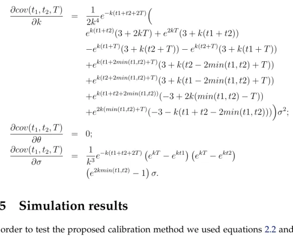
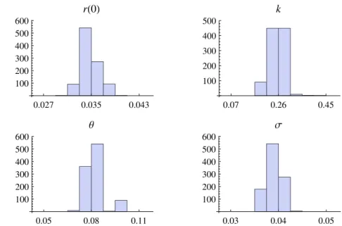
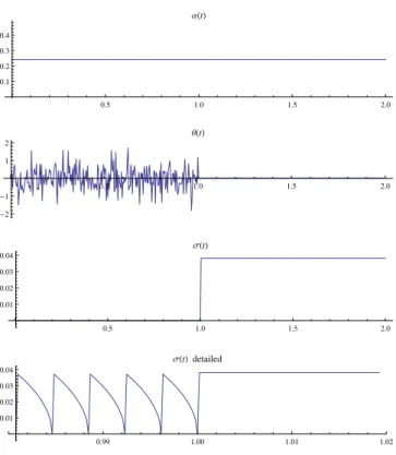
3.1 Prior parameters histograms, learned from simulated data. . . 41 3.2 Short rate SDE deterministic time dependent parametersα(t),θ(t)
andσ(t), for one of the simulated trajectories. . . 42 3.3 Short rate SDE deterministic time dependent parametersα(t),θ(t)
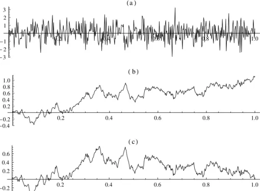
LIST OF FIGURES xviii 4.1 Simulated trajectories of: (a) white noise; (b) the corresponding
Wiener process; (c) the corresponding Brownian bridge. . . 48 4.2 Gaussian processes for machine learning regression with the Wiener
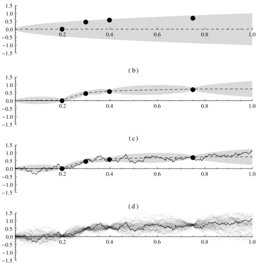
process as prior:(a) prior process mean (dashed), prior process two standard deviations band (gray) and the training set (circles); (b) regression function (dashed) and two standard deviations regres-sion confidence band (gray); (c) training set simulated trajectory; (d) simulated Wiener process trajectories passing through the train-ing set. . . 50 4.3 Brownian bridge trajectories simulated with the vectorial Equation
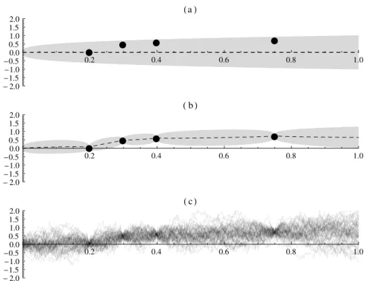
4.17: (a) prior process mean (dashed), prior process two standard deviations band (gray) and the training set (circle); (b) regression function (dashed) and two standard deviation regression confi-dence band (gray); (c) Brownian bridge simulated trajectories. . . . 52 4.4 Gaussian processes for machine learning regression with
geomet-ric Brownian motion as prior: (a) prior process mean (dashed), prior process two standard deviations band (gray) and the train-ing set (circle); (b) regression function (dashed) and two standard deviation regression confidence band (gray); (c) path dependent simulated trajectories (passing through the training set). . . 56 4.5 Gaussian processes for machine learning regression with fractional
Brownian motion as prior: (a) prior process mean (dashed), prior process two standard deviations band (gray) and the training set (circles); (b) regression function (dashed) and two standard devia-tion regression confidence band (gray); (c) path dependent simu-lated trajectories (passing through the training set). . . 57 4.6 Gaussian processes for machine learning regression with the
Ornstein-Ulenbeck mean reversion process as prior: (a) prior process mean (dashed), prior process two standard deviations band (gray) and the training set (circles); (b) regression function (dashed) and two standard deviation regression confidence band (gray); (c) path de-pendent simulated trajectories (passing through the training set). . 58 4.7 2D Wiener process single path representation of a Norbert Wiener
LIST OF FIGURES xix 5.1 VaR computation time line. The gray zone represents the time
in-terval where there are historical prices available. The dashed part of the historical maturities arrows means that those arrows can ex-tend to all the gray zone. . . 64 5.2 VaR computation time line fornV aR= 1. The gray zone represents
the time interval where there are historical prices available. The dashed part of the historical maturities arrows means that those arrows can extend to all the gray zone. . . 67 5.3 Real historical prices of a zero coupon bond with principal P =
1000maturing at dayT = 731. The prices are in percentage of the principal. . . 69 5.4 Daily compounded annualized implied yields from the historical
prices of Exhibit 5.3, as a function of both time and time to maturity. 69 5.5 (a)HR(n= 190, N = 30)historical return maturities. (b) VaR
com-puted at timenV aR = 372relevant maturities. . . 70 5.6 (a)N = 30days market observed historical return at dayn = 190.
(b) Day n = 190 implied yield and future value at time nV aR + N = 402. (c) Dayn = 160implied yield and future value at time nV aR = 372. (d) The adjusted historical return for timenV aR= 372.. 71 5.7 The prices that determine theN = 30days historical return at time
n = 190, the corresponding future prices at timesnV aR = 372 and nV aR +N = 402, along with the historical prices sequence. The arrows represent future values. . . 71 5.8 Step 1– Future valuesv(nV aR+N, n)at timenV aR+N = 402, along
with the historical prices sequence. . . 72 5.9 Step 2 – Future values v(nV aR, n −N)at time nV aR = 372, along
with historical prices sequence. . . 72 5.10 Future valuesv(m, n), at times m = nV aR+N = 402(Step 1) and
m=nV aR = 372(Step 2), along with the historical prices sequence. The future values are plotted as a function of the time n, of the historical pricep(n), that fixed the future value.. . . 73 5.11 Step 3 – Sequence of adjusted historical returns for nV aR = 372
along with the corresponding historical returns sequence.. . . 74 5.12 Adjusted returns for nV aR = 372 and the historical returns
LIST OF FIGURES xx 5.13 Time horizonN = 30, confidence levelα = 99%, bondBVaR,
com-puted at day nV aR = 372 by historical simulation using adjusted historical returns. . . 74 5.14 Step 1– Past values v(nV aR+N, n)at timenV aR+N = 31, along
with the historical prices sequence. . . 75 5.15 Step 2 – Past valuesv(nV aR, n−N)at time nV aR = 1, along with
historical prices sequence. . . 76 5.16 Past valuesv(m, n), at timesm =nV aR+N = 31(Step 1) andm =
nV aR = 1 (Step 2), along with the historical prices sequence. The past values are plotted as a function of the timen, of the historical pricep(n), that fixed the past value.. . . 76 5.17 Step 3– Sequence of adjusted historical returns fornV aR = 1along
with the corresponding historical returns sequence. . . 77 5.18 Adjusted returns fornV aR= 1and the historical returns histograms. 77 5.19 Time horizon N = 30, confidence level α = 99%, bond B VaR,
computed at daynV aR = 1by historical simulation using adjusted historical returns. . . 77
7.1 Euribor rates with maturities of 1, 6 and 12 months, quoted by the Euribor contributor banks in 2007 and 2008. . . 99 7.2 Zero coupon bond log prices with maturities of 1, 6 and 12 months,
computed from the corresponding Euribor rates, quoted by the Eu-ribor contributor banks in 2007 and 2008. . . 100 7.3 Zero coupon bond portfolios log prices with maturities of 1, 6 and
12 months, computed from the corresponding Euribor rates, quoted by the Euribor contributor banks in 2007 and 2008. The number of portfolios at each time and each maturity is 16. Each portfolio price is the average of 24 randomly selected zero coupon bonds, computed from the quoted contributor banks rates. . . 101 7.4 Euribor’s 5 day short rate model zero coupon bond log prices: data
List of Tables
2.1 Parametersr0, k,θ andσ, 1000 calibrations mean, standard
devia-tion and 95% confidence interval. . . 22 2.2 Learned parameters r0, k, θ and σ, for a real, two year maturity,
zero coupon bond, calibrated with approximately one year of avail-able prices. . . 23
3.1 Prior parameters r(0), k, θ and σ, mean, standard deviation and 95%confidence interval, learned from1000simulated data calibra-tions. . . 40 3.2 Euribor model prior parameters, learned from one randomly
se-lected maturity quote per day, from CGD bank, during 2007 and 2008. . . 42
4.1 Iterative and vectorial execution times comparison for the refer-ence task. . . 53 4.2 1000 trajectories execution time sensitivity to the number of samples. 53 4.3 1000 samples per trajectory execution time sensitivity to the
num-ber of trajectories. . . 53
1
Introduction
1.1
Interest rate basics
The financial instrument used in this thesis is the zero coupon bond.
A T-maturity zero coupon bond is a contract that guarantees its holder the payment of one currency unit at timeT. No intermediate payments prior to time
T exist (no coupons). The price at timet < T of theT-maturity zero coupon bond is denoted byp(t, T).
Given three time instantst < S < T, consider the usual construction of con-tracting, at timet, a deterministic rate of return over the periodStoT, using zero coupon bonds, namely (Björk2004):
At timet Sell oneS-maturity zero coupon bond byp(t, S) currency units. With
that amount buyp(t, S)/p(t, T)T-maturity zero coupon bonds. The result-ing net investment at timetequals zero.
At timeS Pay one unit of currency to theS-maturity zero coupon bond holder.
At timeT Receivep(t, S)/p(t, T)currency units for holding theT-maturity zero
coupon bonds.
1. INTRODUCTION 1.2. Calibration problem
compounded interest rateR, over the future periodStoT, which is the solution of:
1eR(T−S)= p(t, S)
p(t, T). (1.1)
Such interest rate is called the continuously compounded forward rate and is given by
R(t, S, T) =−logp(t, T)−logp(t, S)
T −S . (1.2)
Assuming thatp(t, T)is differentiable w.r.t. T, the instantaneous forward rate
f(t, T)is given by
f(t, T) = −∂logp(t, T)
∂T . (1.3)
The instantaneous short rate, or simply the short rate, is defined by
r(t) = f(t, t). (1.4)
The importance of the short rate relies on the fact that on an arbitrage free market, the price, at timet < T, of anyT-maturity contingent claim with payoff Φ(r(T)), is given by
π(t, T) =EQhe−RtTr(s)ds×Φ(r(T)) i
(1.5)
where the expectation is to be taken under the arbitrage free risk neutral mea-sureQ.
In particular, the price of aT-maturity zero coupon bond, in which caseΦ(r(T)) = 1, is given by
p(t, T) = EQhe−RtTr(s)ds i
. (1.6)
1.2
Calibration problem
1. INTRODUCTION 1.2. Calibration problem
0.0 0.2 0.4 0.6 0.8 1.0
0.6 0.7 0.8 0.9 1.0
Figure 1.1: Vasicek zero coupon bond price mean (dashed) and two standard de-viation band (light gray), along with a zero coupon bond prices sequence (solid) available until the current time.
The idea is to model the short rate dynamics directly under the risk neutral measure. This immediately raises the problem of obtaining the models param-eters under the risk neutral measure while fitting the contingent claims prices observed in the market, in particular those of zero coupon bonds.
As noted by (Pang1998) there are relatively few papers dedicated to this prob-lem. Regarding the popular models mentioned above, the only one that explicitly deals with the calibration problem is the Hull-White model.
To illustrate this problem let’s consider a zero coupon bond prices trajectory and the Vasicek short rate model under the risk neutral measure. Under this model zero coupon bond prices are given by
p(t, T) = eA(t,T)−B(t,T)r(t) (1.7)
where A(t, T)and B(t, T)are deterministic functions of the model’s parame-ters. Zero coupon bond prices mean and covariance functions are given by closed forms.
Now suppose that the model parameters were obtained under the risk neutral measure from the zero coupon bond prices trajectory.
Figure 1.1 illustrates both the zero coupon bond prices trajectory and the model’s zero coupon bond prices mean and covariance functions.
The calibration problem can be summarized by the following two issues:
1. As it can be observed in Figure 1.1, the current zero coupon bond model’s price, given by the current model’s mean, does not match the one observed in the market. This situation is quite uncomfortable.
1. INTRODUCTION 1.3. Gaussian processes for machine learning regression
means that the current term structure of interest rates obeys a fixed shape imposed by the model. This situation is highly unrealistic.
An additional description of this problem can be found in (Rainer2009).
1.3
Gaussian processes for machine learning
regres-sion
Given a Gaussian process prior and a set of observations data, Gaussian processes for machine learning regression framework uses the conditional distribution of a Gaussian random vector (T. W. Anderson2003) to construct the posterior process on data. The posterior process on data is the stochastic process whose trajectories are those of the prior process restricted to the ones that pass through the observed data. The posterior process is also Gaussian. Its mean and covariance functions are used as regression and regression confidence functions, respectively.
Consider the Gaussian process priory=g(x)defined by
g(x)∼ GP(m(x), cov(xi,xj)) (1.8)
where the mean and covariance functions, m(x) and cov(xi,xj), are families of functions parametrized by the parameters vectorΦ.
Consider also, data D = (X,y), where matrix X collects a set of vectors
{x⋄1,x⋄2,· · · ,xn⋄}where the value y⋄ = g(x⋄)was observed, and vector ycollects
the corresponding set of observed values{y⋄
1, y2⋄,· · · , yn⋄}.
The posterior Gaussian process on data,y=gD(x), is defined by
gD(x)∼ GP(mD(x), covD(xi,xj)). (1.9)
where mean and covariance function, mD(x) and covD(xi,xj), are given by (Rasmussen2004)
mD(x) = m(x) +K⊤X,xK
−1(y−m) (1.10)
and
covD(xi,xj) = cov(xi,xj)−K⊤X,xiK−1KX,xj. (1.11)
1. INTRODUCTION 1.4. Thesis contribution
æ æ æ
HaL
æ æ æ
HbL
Figure 1.2: (a) A Gaussian process mean (dashed), two standard deviations band (gray) along with some simulated trajectories. (b) the same for the corresponding conditioned on data Gaussian. The conditioning data is a set of samples (dots) of the highlighted trajectory (solid).
Figure 1.2illustrates both the prior process and the conditioned on data pro-cess.
Parameters Φare obtained directly from data by maximizing the prior likeli-hood of the data given the parameters. Given that the process is Gaussian, closed forms of the derivatives of the likelihood w.r.t. each parameter are available and can be used by the maximization procedure.
A natural problem that arises under this framework is the selection of prior mean and covariance functions to use.
1.4
Thesis contribution
The main contribution of this thesis is the proposal of a risk neutral short rate model developed by merging arbitrage free interest rate theory with Gaussian processes for machine learning.
From arbitrage free interest rate theory we use the Vasicek model under the risk neutral measure as prior. Under this model, zero coupon bond log prices are Gaussian. Their mean and covariance functions are given by closed forms.
From Gaussian processes for machine learning we use the conditioned on data regression model. Under this framework the model parameters are learned di-rectly from data and the resulting model automatically fits all the data.
Putting the two pieces together:
1. INTRODUCTION 1.4. Thesis contribution
æ æ
æ æ æ
0.0 0.2 0.4 0.6 0.8 1.0
0.6 0.7 0.8 0.9 1.0
Figure 1.3: One factor machine learning Gaussian short rate model for maturity
T = 1: zero coupon bond prices mean (dashed), two standard deviations band (gray), a zero coupon bond prices sequence (solid), and the conditioning data (dots).
parameters under the risk neutral measure by using the Gaussian processes for machine learning regression, learning parameters from data procedure, with market observed zero coupon log prices;
• we addressed the risk neutral short rate model problem of fitting zero coupon bond prices observed in the market problem by using the Gaussian pro-cesses for machine learning regression conditioned on data model;
• we addressed Gaussian processes for machine learning problem of choos-ing priors mean and covariance functions by uschoos-ing a log normal risk neu-tral short rate model with mean and covariance functions given by closed forms.
The proposed model is a risk neutral measure Vasicek short rate prior condi-tioned on zero coupon bond prices.
All the parameters of the proposed model are obtained directly under the risk neutral measure using market observed zero coupon bond log prices, exclusively. No other data sources are needed.
The model automatically fits, by its construction, all zero coupon bond prices observed in the market, in particular those that define the current term structure of interest rates.
Figure1.3illustrates the proposed model. It is the adaptation of Figure1.2(b) to the setup in Figure1.1(to highlight the conditioning on data mechanism, only a subset of the available zero coupon bond prices is used).
1. INTRODUCTION 1.5. Thesis structure
1.5
Thesis structure
This thesis has two parts. The first part contains a set of self-contained finished papers, one already published, another accepted for publication and the others submitted for publication. The second part contains a set of self-contained unsub-mitted papers. Although the fundamental work on papers in part two is finished as well, there are some extra work we want to include before submitting them for publication.
All the work is supported by a large set of Wolfram Mathematica (Wolfram Research2009) (Wolfram Research2011) (Wolfram Research2012) packages and notebooks. Facing the impossibility to present all those program in this thesis, we have chosen to include in AppendixAthe public sections of two core packages, one symbolic and another numeric.
Part I
Machine learning Vasicek model calibration with Gaussian
pro-cesses
This paper was the first step towards merging arbitrage free short rate theory with Gaussian processes for machine learning regression.
Using the zero coupon bond log prices of a singleT-maturity bond, we have obtained the values of the Vasicek short rate model parameters directly under the risk neutral measure.
The main contributions of this paper are:
• Obtain the Vasicek zero coupon bond log prices mean and covariance func-tions closed forms;
• Show, by simulation, that the risk neutral model parameters are properly obtained from the zero coupon bond log prices, by maximizing the likeli-hood of the log prices given the parameters;
1. INTRODUCTION 1.5. Thesis structure
One Factor Machine Learning Gaussian Short Rate
In this paper we have recognized the conditioned on zero coupon bonds log prices short rate model, with the Vasicek short rate model as prior, as an alter-native short rate model by itself.
The main contributions of this paper are:
• Obtain the model’s deterministic time dependent stochastic differential equa-tion parameters;
• Show, by simulation, that the risk neutral model parameters are properly obtained from several zero coupon bond log prices with distinct maturities, by maximizing the likelihood of the log prices given the parameters, as long as there is only one price observation in each time instant.
Brownian Bridge and other Path Dependent Gaussian Processes
Vectorial Simulation
Both the iterative and the vectorial procedures for simulating the Wiener pro-cess are widely known, and described in reference books such as Glasserman 2003. However, regarding the Brownian bridge, only the iterative procedure is described.
In this paper we model the Brownian bridge using the Gaussian processes for machine learning regression framework, using the Wiener process, W(t), as prior, and the single observation, W(1) = 0, the Brownian bridge condition, in the training set.
The main contributions of this paper are:
• Use the bridge mean vector and the covariance matrix, computed in a set of sampling instants, to simulate the bridge trajectories with the same vectorial procedure used to simulate any Gaussian vector;
• Extend the vectorial simulation procedure to other Gaussian processes pri-ors, and for more than one conditions, by developing a general path depen-dent Gaussian process trajectories vectorial simulation framework;
1. INTRODUCTION 1.5. Thesis structure
Bonds Historical Simulation Value at Risk
In several simulation situations spread across this thesis, in order to evaluate the existence of numerical problems, we have scaled zero coupon bond prices by using the implied yield at a certain time, to compute the bond price at another time, assuming the bond was held to maturity (mark to model).
This scaling procedure proved to be an important tool in the context of histor-ical simulation value at risk (VaR) for portfolios with bonds.
In a joint work with Prof. Manuel Esquível and Prof. Pedro Corte Real, we have sold the authors wrights of an historical simulation value at risk implemen-tation, for portfolios with bonds (among other securities), to a private bank, by 50.100,00 EUR. That implementation was based on this paper.
The main contributions of this paper are:
• Adjust bonds historical returns so that the adjusted returns can be used di-rectly to compute VaR by historical simulation;
• Using real bond prices, to show that the developed method provides results consistent with the usual market observed trend, in which shorter times to maturity imply smaller yields, carrying smaller risk and consequently having smaller VaR;
• Using real bond prices, to show that the developed method strongly pre-serves the market implicit correlations between the instruments in the port-folio.
Part II
Machine Learning Gaussian Short Rate
Using a single Vasicek short rate factor, under the risk neutral measure, the ma-chine learning Gaussian short rate model can’t solve the term structure fitting issue mentioned in Section1.2. In this paper a sum of Vasicek short rate factors is proposed in order to solve that problem.
The main contributions of this paper are:
• Propose a sum of Vasicek short rate factors, under the risk neutral measure, as a prior to Gaussian processes for machine learning regression;
1. INTRODUCTION 1.5. Thesis structure
Interest Rate Market Changes Detection
A common problem that arises in mathematical finance when using models with parameters estimated from market data, available until a certain time, is that of checking the necessity of using new parameters as newer data become available. In this paper we use a covariance matrix statistical test to evaluate the neces-sity of using new parameters of a machine learning Gaussian short rate model of the Euribor, as newer data become available. Whenever we detect such necessity, we say that the market conditions have changed.
The main contributions of this paper are:
• Obtain the likelihood ratio criterion to test if a covariance matrix,Σ, is equal to a given matrix,Σ0, as a decomposition of simpler tests.
• Propose a machine learning Gaussian short rate model with Vasicek short rate noise in the observations.
Part I
2
Machine learning Vasicek model
calibration with Gaussian processes
2.1
Preamble
With the exception of this preamble and minor notation changes, this chapter con-tains the paper Machine learning Vasicek model calibration with Gaussian processes, joint work with Prof. Manuel Esquível and Prof. Raquel Gaspar, published in journal Communications in Statistics-Simulation and Computation, volume 41, number 6, pages 776 to 786, year 2012, by Taylor & Francis.
This paper was the first step towards merging arbitrage free short rate theory with Gaussian processes for machine learning regression.
Using the zero coupon bond log prices of a singleT-maturity bond, we have obtained the values of the Vasicek short rate model parameters directly under the risk neutral measure.
The main contributions of this paper are:
• Obtain the Vasicek zero coupon bond log prices mean and covariance func-tions closed forms;
2. VASICEK CALIBRATION 2.2. Introduction
• Calibrate the model for a real zero coupon bond.
Abstract
In this paper we calibrate the Vasicek interest rate model under the risk neutral measure by learning the model parameters using Gaussian processes for machine learning regression. The calibration is done by maximizing the likelihood of zero coupon bond log prices, using mean and covariance functions computed analyt-ically, as well as likelihood derivatives with respect to the parameters. The max-imization method used is the conjugate gradients. We stress that the only prices needed for calibration are market observed zero coupon bond prices and that the parameters are directly obtained in the arbitrage free risk neutral measure.
Keywords: Vasicek interest rate model; Arbitrage free risk neutral measure;
Calibration; Gaussian processes for machine learning; Zero coupon bond prices.
2.2
Introduction
Calibration of interest rate models under the risk neutral measure typically entails the availability of some derivatives such as swaps, caps or swaptions.
In this paper we present an alternative method for calibrating Gaussian mod-els, namely, the Vasicek interest rate model (Vasicek 1977), which requires zero coupon bond prices only.
The presented method has the following features:
• The only prices needed for calibration are zero coupon bond prices.
• All the model parameters are directly obtained in the risk neutral measure.
• The calibration method does not require a discrete model approximation nor the establishment of an objective measure dynamics.
The method is based on Gaussian processes for Machine Learning, and its main drawback is his applicability to Gaussian models only.
2. VASICEK CALIBRATION 2.3. Vasicek interest rate model
into a Gaussian process by taking the logarithm of the zero coupon prices. The mean and covariance functions of this Gaussian process can be computed analyt-ically making it suitable for Gaussian processes for machine learning regression.
2.3
Vasicek interest rate model
In the Vasicek model, the interest rate follows an Ornstein-Uhlenbeck mean-reverting process, under the risk neutral measure, defined by the stochastic dif-ferential equation
dr(t) =k(θ−r(t))dt+σdW(t) (2.1)
where k is the mean reversion velocity,θ is the mean interest rate level, σ is the volatility andW(t)the Wiener process. Parameterskandσare positive.
Lets≤t. The solution of equation2.1is (Brigo and Mercurio2006)
r(t) = r(s)e−k(t−s)+θ 1−e−k(t−s)+σe−kt
Z t
s
ekudW(u). (2.2)
The interest rater(t), conditioned onFs, is normally distributed with mean
E{r(t)|Fs}=r(s)e−k(t−s)+θ 1−e−k(t−s)
(2.3)
and variance
V ar{r(t)|Fs}=
σ2
2k 1−e
−2k(t−s).
Zero coupon bonds are interest rate derivatives, therefore, their market prices are observed in the risk neutral measure. The Vasicek model has affine term struc-ture, which means that theT maturity zero coupon bond pricesp(t, T), observed in the risk neutral measure, are given by (Björk2004)
p(t, T) = eA(t,T)−B(t,T)r(t) (2.4)
where
A(t, T) =
θ− σ
2
2k2
(B(t, T)−T +t)− σ
2
4kB
2(t, T)
and
B(t, T) = 1
k 1−e
2. VASICEK CALIBRATION 2.3. Vasicek interest rate model
Equation 2.4 shows that the zero coupon bond pricesp(t, T) are log normal and consequentlylog(p(t, T))are normal.
2.3.1
Zero coupon bond log prices mean function
Since
log(p(t, T)) =A(t, T)−B(t, T)r(t) (2.5)
the mean functionµ(t, T)oflog(p(t, T))is given by
µ(t, T) = E{log(p(t, T))|Fs}
= E{A(t, T)−B(t, T)r(t)|Fs} = A(t, T)−B(t, T)E{r(t)|Fs}
Considering the initial instant s = 0, and using equation 2.3 for E{r(t)|Fs} we get
µ(t, T) = A(t, T)−B(t, T) r0e−kt+θ 1−e−kt
=
θ− σ
2
2k2 t−T −
ek(t−T)−1
k
− σ
2 ek(t−T)−12
4k3
−e
−kT ek(T−t)−1 θ ekt−1+r
0
k (2.6)
wherer0stands for the initial interest rate value, the value of the interest rater(t),
att= 0.
2.3.2
Zero coupon bond log prices covariance function
The covariance functioncov(t1, t2, T)oflog(p(t, T))is given by
cov(t1, t2, T) = E{(log(p(t1, T))−µ(t1, T))
(log(p(t2, T))−µ(t2, T))|Fs}
2. VASICEK CALIBRATION 2.3. Vasicek interest rate model
Using equation2.5, the termE{log(p(t1, T)) log(p(t2, T))|Fs}, is given by
E{log(p(t1, T)) log(p(t2, T))|Fs} = E{(A(t1, T)−B(t1, T)r(t1))
(A(t2, T)−B(t2, T)r(t2))|Fs} = A(t1, T)A(t2, T)
−A(t1, T)B(t2, T)E{r(t2)|Fs}
−B(t1, T)A(t2, T)E{r(t1)|Fs}
+B(t1, T)B(t2, T)E{r(t1)r(t2)|Fs} (2.8)
Using the Vasicek SDE solution equation2.2, withs = 0, the termE{r(t1)r(t2)|Fs} is given by
E{r(t1)r(t2)|Fs}
= E
r0e−kt1 +θ 1−e−kt1
+σe−kt1
Z t1
0
ekudW(u)
r0e−kt2 +θ 1−e−kt2
+σe−kt2
Z t2
0
ekudW(u)
= r20e−k(t1+t2)+r0e−kt1θ 1−e−kt2
+θ 1−e−kt1r
0e−kt2 +θ2 1−e−kt1
1−e−kt2
+σ2e−k(t1+t2)E
Z t1
0
ekudW(u)
Z t2
0
ekudW(u)
. (2.9)
In order to computeEnRt1
0 e
kudW(u)Rt2
0 e
kudW(u)o, we first considert
1 < t2.
In this case, we have
E
Z t1
0
ekudW(u)
Z t2
0
ekudW(u)
= E
Z t1
0
ekudW(u)
Z t1
0
ekudW(u) +
Z t2
t1
ekudW(u)
= E
(Z t1
0
ekudW(u)
2)
2. VASICEK CALIBRATION 2.4. Gaussian processes for machine learning
In caset2 < t1, we have
E
Z t1
0
ekudW(u)
Z t2
0
ekudW(u)
= E
Z t2
0
ekudW(u) +
Z t1
t2
ekudW(u)
Z t2
0
ekudW(u)
= E
(Z t2
0
ekudW(u)
2)
. (2.11)
Given equations2.10and2.11, we get
E
Z t1
0
ekudW(u)
Z t2
0
ekudW(u)
= E
Z min(t1,t2)
0
ekudW(u)
!2
.
Finally, using Itô isometry
E
Z t1
0
ekudW(u)
Z t2
0
ekudW(u)
= E
Z min(t1,t2)
0
ekudW(u)
!2
=
Z min(t1,t2)
0
En eku2odu
=
Z min(t1,t2)
0
e2kudu
= 1 2k e
2k min(t1,t2)−1. (2.12)
Using equations2.6,2.7,2.8,2.9and2.12, the covariance functioncov(t1, t2, T)
oflog(p(t, T))is given by
cov(t1, t2, T) =
1 2k3e
−k(2T+t1+t2) e2k min(t1,t2)
−1
ekT −ekt1 ekT −ekt2σ2 (2.13)
2.4
Gaussian processes for machine learning
2. VASICEK CALIBRATION 2.4. Gaussian processes for machine learning
functions1(Rasmussen and Williams2005)
GP ∼ N(µ(x), cov(x1,x2)).
The pair (X,y) is the training set. The matrix X collects a set ofn vectors x
where the valuey=f(x)was observed. The correspondingyvalues are collected in vectory.
The set of vectorsx⋆ where the valuesy⋆ = f(x⋆)were not observed, is col-lected in matrixX⋆. The matrixX⋆ is the test set.
Under the Vasicek interest rate model the zero coupon bonds log priceslog(p(t, T)) are normal
GP ∼ N(µ(t, T), cov(t1, t2, T))
whereµ(t, T)is given by equation2.6andcov(t1, t2, T)is given by equation2.13.
SinceT, the bond maturity, is a bond feature, in this case the mapping we are interested in is the scalar mapping
y=f(t)
where y stands for the zero coupon bonds log prices. This reduces the training set to the pair of vectors(t,y), and the test set to vectort⋆.
Since the process is Gaussian (Rasmussen and Williams2005)
" y
y⋆ #
∼ N
" µ
µ⋆
#
,
"
K K⋆
KT⋆ K⋆⋆
#!
and
p(y⋆|t⋆,t,y)∼ N µ⋆+KT⋆K−1(y−µ),K⋆⋆−KT⋆K−1K⋆
whereµandµ⋆ are mean vectors of train and test sets, Kis the train set
covari-ance matrix, K⋆ the train-test covariance matrix and K⋆⋆ the test set covariance matrix.
The conditional distribution
p(y⋆|t⋆,t,y)
1See (Rasmussen2004) for a short introduction to the Gaussian distributions over functions
2. VASICEK CALIBRATION 2.4. Gaussian processes for machine learning
corresponds to the posterior process on the data
GPD ∼ N(mD(t), covD(t1, t2))
where
mD(t) =m(t) +KtT,tK−1(y−µ) (2.14)
and
covD(t1, t2) = cov(t1, t2)−KTt,t1K−1Kt,t2 (2.15)
whereKt,tis a covariance vector between every training instant andt.
Equation 2.14is the regression function while equation2.15 is the regression confidence. Equations 2.14 and 2.15 are the central equations of Gaussian pro-cesses for machine learning regression.
In order to learn the model parametersΘ = {r0, k, θ, σ}from data, the
likeli-hood of the training data given the parameters (closed form) (Rasmussen2004)
L = logp(y|t,Θ) = −1
2log|K| − 1
2(y−µ) T
K−1(y−µ)−n
2 log(2π)
is maximized, based on the derivatives ofLwith respect to each of the parameters (closed forms).
Note that, since we want to learn the parameters in the arbitrage free risk neutral measure, the initial interest rate valuer0, is considered a parameter, like
k,θandσ, to be learned from the zero coupon bond log prices. Denoting each of the parameters in setΘbyΘi, and since
∂
∂Θi log|K|=tr
K−1∂K
∂Θi
and
∂ ∂ΘiK
−1 =−K−1∂K
∂ΘiK
2. VASICEK CALIBRATION 2.4. Gaussian processes for machine learning
the derivatives ∂∂LΘ
i are given by
∂L
∂Θi = − 1 2tr
K−1∂K
∂Θi
+1
2(y−µ) T
K−1∂K
∂ΘiK
−1(y−
µ)
+ (y−µ)T K−1 ∂µ
∂Θi.
In order to compute the vector of derivatives, ∂µ
∂Θi, and the matrix of
deriva-tives ∂∂ΘKi, the derivatives of the mean function µ(t, T) (equation 2.6), and the derivatives of the covariance function cov(t1, t2, T) (equation 2.13) with respect
to the parameters are used, namely:
∂µ(t, T)
∂r0
= e
−kT −e−kt
k ;
∂µ(t, T)
∂k =
e−k(t+2T)
4k4 4k
2(kt+ 1)e2kT(r
0−θ)
−4k2(kT + 1)(r0−θ)ek(t+T)+ 4σ2ek(2t+T)(k(t−T)−3)
−σ2e3kt(2k(t−T)−3) +σ2ek(t+2T)(4k(t−T) + 9);
∂µ(t, T)
∂θ =
e−kt−e−kT +kt−kT
k ;
∂µ(t, T)
∂σ = −
σ 2k(t−T)−4ek(t−T)+e2k(t−T)+ 3
2k3 ;
∂cov(t1, t2, T)
∂r0
2. VASICEK CALIBRATION 2.5. Simulation results
∂cov(t1, t2, T)
∂k =
1 2k4e
−k(t1+t2+2T)
ek(t1+t2)(3 + 2kT) +e2kT(3 +k(t1 +t2))
−ek(t1+T)(3 +k(t2 +T))−ek(t2+T)(3 +k(t1 +T)) +ek(t1+2min(t1,t2)+T)(3 +k(t2−2min(t1, t2) +T)) +ek(t2+2min(t1,t2)+T)(3 +k(t1−2min(t1, t2) +T))
+ek(t1+t2+2min(t1,t2))(−3 + 2k(min(t1, t2)−T)) +e2k(min(t1,t2)+T)(−3−k(t1 +t2−2min(t1, t2)))σ2;
∂cov(t1, t2, T)
∂θ = 0;
∂cov(t1, t2, T)
∂σ =
1
k3e
−k(t1+t2+2T) ekT
−ekt1 ekT −ekt2
e2kmin(t1,t2)−1σ.
2.5
Simulation results
In order to test the proposed calibration method we used equations2.2 and 2.5, with fixed parameters values, to simulate 1000 sequences of zero coupon bond log prices.
The parameters values used were: initial interest rater0 = 0.5; mean interest
rate levelθ = 0.1; mean reversion velocityk = 2; and volatilityσ= 0.2.
We considered the zero coupon bond maturity of one year,T = 1, and simu-lated one year daily prices sequences by considering 260 prices per sequence (5 working days prices per week, 52 weeks per year).
Figure2.1illustrates a simulated sequence of zero coupon bond log prices, as well as the mean and variance functions.
We applied the calibration procedure by maximizing the likelihood of each one of the zero coupon bond log prices sequences, using Wolfram Mathematica 7 (Wolfram Research2009) conjugate gradients implementation with default con-figuration parameters.
Figure 2.2 illustrates the 50 bins parameters histograms obtained from the 1000 calibrations performed, and Table2.1 shows the corresponding mean, stan-dard deviation and 95% confidence intervals.
2. VASICEK CALIBRATION 2.5. Simulation results
0.0 0.2 0.4 0.6 0.8 1.0 -0.25
-0.20 -0.15 -0.10 -0.05 0.00
TimeHin yearsL
Zero
coupon
bond
log
price
Figure 2.1: Zero coupon bond log prices simulated sequence (solid black), mean (dashed black) and two standard deviations interval (light gray).
0.0 0.5 1.0 1.5
20 40 60 80 100 120 140
r0
1 2 3 4 5
20 40 60 80 100 120
k
-0.4-0.2 0.0 0.2 0.4 20
40 60 80
Θ
0.15 0.20 0.25 0.30
20 40 60 80 100
Σ
Figure 2.2: Learned parameters 50 bins histograms.
Parameter Value Mean Std. Dev. 95% CI
r0 0.5 0.527 0.482 -0.418 to 1.472
k 2.0 2.098 0.855 0.419 to 3.776
θ 0.1 0.083 0.443 -0.786 to 0.952
σ 0.2 0.203 0.039 0.126 to 0.280
Table 2.1: Parametersr0, k, θ and σ, 1000 calibrations mean, standard deviation
2. VASICEK CALIBRATION 2.6. Calibration to real data
r0 k θ σ
Learned 0.212 2.925 0.025 0.195 Std. Dev. 0.110 1.897 0.022 0.119
Table 2.2: Learned parameters r0, k, θ and σ, for a real, two year maturity, zero
coupon bond, calibrated with approximately one year of available prices.
means showed in third column of Table2.1, are quite accurate, the confidence in-tervals for each individual calibration are quite large. Therefore calibration with the proposed method should include as much zero coupon bond prices sequences as possible. Care should be taken when calibrating the model with just one price sequence, because the estimation errors can be quite large.
2.6
Calibration to real data
In real life there are only a few zero coupon bonds and their great majority is traded over the counter (OTC). Those bonds are traded between two market play-ers instead of openly being traded in an exchange and data is scarce. Zero coupon bond prices can also be implicitly extracted from the prices of other fixed income products, but in this case the prices would be theoretical and dependent on the assumptions underlying the term structure fitting.
We had, thus, two choices: either use actual market data on one of the few zero coupon bonds actually traded on the market and rely on OTC quotes, or use the price on other fixed income products and extract from those theoretical zero coupon bond prices. We chose the first approach. At the time we looked for data there was a two year maturity zero coupon in the OTC market live for approximately one year. We took this bond and used a quote service that delivers market prices aggregated from different dealers responsible for trading (market makers) this particular bond.
Table 2.2 shows the parameters learned and standard deviations obtained from the square root of the diagonal of the inverse Fisher information matrix, as a measure of the calibration errors. Figure 2.3 illustrates the corresponding mean and variance functions, along with the log prices sequence itself. It should be noted that the learned parameters along with equations2.14and2.15allow the plot in Figure2.3 of the learned mean and the learned two standard deviations interval, not only in the time interval where there are available prices, but for the alltbetween the initial timet= 0and maturityt=T.
2. VASICEK CALIBRATION 2.7. Conclusions
0.0 0.5 1.0 1.5 2.0
-0.10 -0.08 -0.06 -0.04 -0.02 0.00
TimeHin yearsL
Zero
coupon
bond
log
price
Figure 2.3: Real, two year maturity, zero coupon bond log prices sequence (solid black), learned mean (dashed black) and learned two standard deviations interval (light gray).
deviations obtained do confirm that the errors in the learned parameters can be quite large when calibrating with just one price sequence.
2.7
Conclusions
In this paper we presented a calibration procedure of the Vasicek interest rate model under the risk neutral measure by learning the model parameters using Gaussian processes for machine learning regression with zero coupon bond log prices mean and covariance functions computed analytically.
3
One Factor Machine Learning
Gaussian Short Rate
3.1
Preamble
With the exception of this preamble and minor notation changes, this chapter con-tains the paperOne Factor Machine Learning Gaussian Short Rate, joint work with Prof. Manuel Esquível and Prof. Raquel Gaspar, which is submitted for publi-cation in the journal Communipubli-cations in Statistics-Simulation and Computation, by Taylor & Francis. The current submission status is "under revision".
In this paper we have recognized the conditioned on zero coupon bonds log prices short rate model, with the Vasicek short rate model as prior, as an alterna-tive short rate model by itself.
The main contributions of this paper are:
• Obtain the model’s deterministic time dependent stochastic differential equa-tion parameters;
3. ONEFACTOR 3.2. Introduction
Abstract
In this paper we model the short rate, under the risk neutral measure, as a Gaus-sian process, conditioned on market observed zero coupon bonds log prices. The model is based on Gaussian processes for machine learning, using a single Va-sicek factor as prior.
All model parameters are learned directly under the risk neutral measure, using zero coupon bonds log prices only.
The model supports observations of zero coupon bounds with distinct matu-rities limited to one observation per time instant. All the supported observations are automatically fitted.
We derive the model’s SDE and model the Euribor using real data.
Keywords: Gaussian short rate, Gaussian processes for machine learning, risk
neutral measure.
3.2
Introduction
In our previous work (Sousa, Esquível, and Gaspar2012) we calibrated the Va-sicek (VaVa-sicek1977) short rate model, for a singleT maturity zero coupon bond, directly under the risk neutral measure, using zero coupon bond prices only. The method is based on conditioning the Vasicek zero coupon bond log prices Gaus-sian process, to market observed zero coupon bond log prices, using the GausGaus-sian processes for Machine Learning framework (Rasmussen and Williams2005). In this paper we recognize the conditioned on market observed zero coupon log prices underlying Gaussian process as an alternative one factor Gaussian short rate model by itself. We extend the calibration method to several T maturity zero coupon bonds, limited to one observation per time instant, and derive the model’s stochastic differential equation.
Consider the Gaussian processg(x), with mean functionm(x)and covariance functioncov(xi,xj),
g(x)∼ GP(m(x), cov(xi,xj)). (3.1)
Consider also, data D = (X,y), where the matrix X collects a set of vectors
{x⋄1,x⋄2,· · · ,xn⋄}where the value y⋄ = g(x⋄)was observed, and vector ycollects
the corresponding set of observed values{y⋄
3. ONEFACTOR 3.3. Short rate prior
The process,gD(x), defined by all trajectories ofg(x)that pass through dataD
is also Gaussian (Rasmussen and Williams2005), with mean functionmD(x)and
covariance functioncovD(xi,xj),
gD(x)∼ GP(mD(x), covD(xi,xj)). (3.2)
The processg(x)is called the prior,gD(x)is called the conditioned on data
pro-cess,Dis called the training set andmD(x),covD(xi,xj)are given by (Rasmussen 2004)
mD(x) = m(x) +KX⊤,xK−1(y−m) (3.3)
and
covD(xi,xj) =cov(xi,xj)−K⊤X,xiK
−1K
X,xj (3.4)
where,mis the prior training set mean vector, Kis the prior training set co-variance matrix and KX,x is a prior covariance vector between every training vector andx.
The "One Factor Machine Learning Gaussian Short Rate" is a single factor ar-bitrage free Vasicek short rate prior, conditioned on market observed zero coupon bonds log prices.
3.3
Short rate prior
The model’s prior is that, under the arbitrage free, risk neutral measure, the short rate,r(t), follows a Vasicek Ornstein-Uhlenbeck mean-reverting process, defined by the stochastic differential equation (SDE) (Vasicek1977):
dr(t) =k(θ−r(t))dt+σdW(t). (3.5)
Parameter k is the mean reversion velocity, parameter θ is the mean interest rate level, parameterσis the volatility andW(t)is the Wiener process. Parameters
kandσare strictly positive.
Lets be the initial time, with0 < s < t. The solution of Equation3.5 is given by (Brigo and Mercurio2006)
r(t) = r(s)e−k(t−s)+θ(1−e−k(t−s)) +σe−kt
Z t
s
3. ONEFACTOR 3.3. Short rate prior
The initial short rate value, r(s), is considered as an extra model parameter since its value must be obtained under the risk neutral measure.
3.3.1
Short rate mean and covariance
Given Equation3.6the short rate prior mean and covariance functions,mr(t)and
covr(t1, t2), are given by
mr(t) =r(s)e−k(t−s)+θ(1−e−k(t−s)) (3.7)
and
covr(t1, t2) =σ2e−k(t1+t2)
1 2k e
2kmin(t1,t2)−e2ks. (3.8)
3.3.2
Zero coupon bond log prices mean and covariance
Under the risk neutral measure, the pricep, at timet, of a zero coupon bond that pays1at maturityT, is given by (Björk2004)
p(t, T) = Ehe−RtTr(u)du i
. (3.9)
Under the Vasicek modelp(t, T)is given by
p(t, T) = eA(t,T)−B(t,T)r(t) (3.10)
where
B(t, T) = 1
k 1−e
−k(T−t) (3.11)
and
A(t, T) =
θ− σ
2
2k2
(B(t, T)−T +t)− σ
2
4kB
2(t, T). (3.12)
It is clear from Equation3.10that model has an affine term structure and that the logarithm of the zero coupon bonds prices is Gaussian
3. ONEFACTOR 3.4. One Factor Machine Learning Gaussian Short Rate
Since the logarithm of zero coupon bonds prices is given by
logp(t, T) = A(t, T)−B(t, T)r(t) (3.14)
the mean and covariancemp(t, T)andcovp(t1, T1, t2, T2)are given by
mp(t, T) = A(t, T)−B(t, T)mr(t) (3.15)
=
θ− σ
2
2k2
1−e−k(T−t)
k −T +t
−σ
2 1−e−k(T−t)2
4k3
− 1−e
−k(T−t) r(s)e−k(t−s)+θ 1−e−k(t−s)
k (3.16)
and
covp(t1, T1, t2, T2)
= B(t1, T1)B(t2, T2)covr(t1, t2) (3.17)
= σ
2e−k(t1+t2) 1−e−k(T1−t1) 1−e−k(T2−t2) e2kmin(t1,t2)−e2ks
2k3 . (3.18)
3.4
One Factor Machine Learning Gaussian Short Rate
Let:
• x= [t T]⊤;
• y= logp(x) = logp(t, T);
• mp(x) =mp(t, T);
• covp(xi,xj) =covp(ti, Ti, tj, Tj).
Following Section3.2, let matrixXcollect a set of vectorsx⋄where the values
of zero coupon log prices were observed, and let vectorycollect the correspond-ing valuesy⋄ = logp(x⋄). Recall from Section3.2 thatD = (X,y)is the training