1
Macroeconomic Constraints to Growth of Brazilian economy Diagnosis and some policy proposals*
José Luis Oreiro** Lionello Punzo*** Eliane Araújo**** Gabriel Squeff***** Abstract: The recent process of accelerated expansion of the Brazilian economy was driven by exports and fixed capital formation. Although the pace of growth was more robust than in the 1990´s, we can still witness the existence of certain macroeconomic constraints to its continuation in the long run such as, for instance, the exchange rate overvaluation in particular since 2005, and in general the modus operandi of monetary policy. Such constraints may jeopardize the sustainability of the current pace of growth. Therefore, we argue that Brazil still lies in a trap made up of high interest and low exchange rates. The elimination of the exchange rate misalignment would bring about a great increase in the rate of interest, which on its turn would impact negatively upon investment and hence upon the sustainability of long run economic growth. We outline a set of policy measures to eliminate such a trap, in particular, the adoption of an implicit target for the exchange rate, capital controls and the abandonment of the present regime of inflation targeting. Recent events seem to go in this direction.
Keywords: Brazil’s growth experience, exchange rate misalignment, de-industrialization
2 1 –Introduction
In the last 20 years the Brazilian economy averaged an annual growth rate of only 0.7% in per capita terms, well below the value of about 3% it reached between 1950 and 1980. Performance was also below that of similar emerging countries like South Korea, China, Mexico and Chile. If it were to continue at such a speed, Brazil would need about 100 years to double per capita income, and even so it would never reach anything near the standard of living of the present developed countries.
The main factors for low growth in the last 20 years are well known. We can pinpoint two fundamental disequilibrium in the economy, which in a long run perspective account for its semi-stagnation. On one side, there is a progressively increasing internal disequilibrium, as a result of the attempt to cope with inflation via mechanisms of price and wage indexation, which have contributed to maintain inflation high and with a persistent tendency to accelerate. Only the “Plano Real” managed to curbe down the inflationary tendency, at least partially. At the same time, domestic disequilibrium was reduced by means of a monetary policy that was excessively conservative, to the effect of keeping the country’s rates of interest among the highest in the world, at the same time as generating the currency appreciation in the period between 1994 and 1998.
3
The last four years have witnessed an acceleration of the growth of the Brazilian
economy as compared to the years after 1988. The average growth rate of the period
2004-2007 was around 4,5%, well above the average performance during any othe previous period: 2000-2003 (2,35% p.a.), 1996-1999 (1,45% p.a), 1992-1995 (3,48%) and 1988-1991 (-0,05%). Assuming an annual growth of population in the order of 1,5%, that GDP growth rate will imply that income per capita in Brasil will return to grow at an annual rate of 3%, thus recovering the levels of performance of the 1950-80 period.
The acceleration of growth was made possible by a combination of two elements: a strong increase in the growth rate of exports since 2000, which proved to be fundamental in acelerating the pace at which aggregate autonomous demand was growing, pushing in this way growth of production, and a relevant increase in the rate of gross fixed capital formation since 2004. This latter contributed significantly to an increase of output, for it allowed the production capacity to adjust to the rate of expansion of aggregate demand.
Fig.1 shows the evolution of the growth rates of GDP, Exports and Gross Fixed Capital Formation during 1996-2007. One can see that the relative deceleration occurred in 1996-99 compared to 1992-95, was accompanied by a remarkable reduction in the growth rate of exports (falling from an annual average growth of 7,55%, down to 5.3%) and by the stagnation of expenditure in gross fixed capital (its average annual rate from 6.7% down to a mere 0.12%). Moreover, the rapid acceleration of growth during 2004-07 was realised as, on the one hand, the growth rate of exports also accelerated compared to its values during the 1990 decade, on the other, the rate of gross fixed capital formation showed a pronounced increase, with values almost doubling those of the rate of growth of real output.
4
The objective of this article is mainly an empirical one. We want to evaluate the sustainability of the growth pace of the Brazilian economy in the period 2004-8. In particular, we try to pinpoint those sources of fragility that could lead to a sudden and sharp reduction in the expansion of exports and in the growth rate of gross fixed capital accumulation, causing a collapse of the current expansion pattern. The main contribution of the paper is to show that the growth pace of the Brazilian economy has at least two macroeconomic sources of fragility, one related to the exchange rate and another related to the short-term interest rate. These sources are responsible for the existence of a “high interest rate-low exchange rate trap”.
The first source is the remarkable exchange rate misalignment, especially since 2005. In contrast to what was recently put forward by Brazilian economists with an orthodox viewpoint, we think that the real exchange rate appreciation in recent years is not due to a reduction in its equilibrium value, but is related to its over-evaluation with respect to such a value.
A second source of fragility, which could have been operating for various years, is related with the inefficacy of monetary policy. Notwithstanding the fall in the rate of interest, Brazil’s levels are still among the highest in the world, both in nominal and real terms. High interest rates over a long period of time have been among the results of the low efficacy of monetary policy. It is the consequence of such inefficacy that convergence of the inflation rate to its chosen long term target requires comparatively higher real interest rates. At the root of that inefficacy are the characteristics of the reaction function of the Brazilian Central
Bank. In our interpretation of the determination of the basic rate, the SELIC, the BCB’s
5
bias towards overreacting affects sensibly gross fixed capital formation and through it the pace of long run growth.
Our interpretative framework is one where growth is driven also in the long run by the dynamics of demand, a well known approach for which we can refer to classic treatments. Next section states our main thesis, namely that the natural growth rate of the Brazilian economy is endogenous while supply conditions do not represent binding constraints to its expansion. In our estimations, such a rate reacts to changes in aggregate demand, ranging between annual values of 5,2% and 8% , this latter of the boom years.
Section 2 analyzes the dynamics of the real exchange rate between 1994-2007; allowing us to draw the conclusion that in the last 14 years it has been chronically misaligned relative to its equilibrium value, with periods of over-evaluation (1994-1998; 2005-2007) alternating with periods of near-equilibrium (1999-2004).
We then move on to analyze the long run effects of such misalignment. We argue that on one side the exchange rate over-evaluation is driving the reappearance of current account deficits, and on the other, it is exerting a negative effect upon long run economic performance. It is also conspiring to induce a desindustrialization process, in the form of a progressive concentration of the country’s production structure into sectors with low contribution to long run sustainable growth.
In Section 4, we reconstruct the dynamics of the determination of short term interest rates with the view of exhibiting the excessive preoccupation by the BCB for inflation, this being one of the sources of the low efficacy of its policy.
6
high short-term interest rate and an over-valued exchange rate, the so-called high interest rate-low exchange rate trap”.
In section 6 we present some policy proposals aimed at reducing and possibly eliminating the factors of fragility inbuilt in the present pace of growth.
Section 7 concludes the paper.
1 – Empirical evidence for the thesis of the endogeneity of the natural growth rate in the Brazilian economy
Hereafter, we begin by looking at the natural rate of growth (NGR) to argue that there is strong evidence for its endogeneity in the case of the Brazilian economy. Our estimates, based on quarterly data for growth and employment between 1980-2002,1 indicate that the natural rate reacts to changes in aggregate demand, and thus the constraints to growth come basically from constraints to aggregate demand expansion, instead of supply conditions2.
The empirical methodology to test for the hypothesis of endogenously or demand- driven growth was pioneered by Ledesma and Thirwall, 20023. Using Okun’s notion of natural rate of growth, (gn) is defined as such rate that corresponds to a constant unemployment level. In fact, Okun specifies the (per cent) change in unemployment as
%U a b g
(1)
Where: U is the unemployment level and g the rate of growth of output. Hence, when %U = 0, the (natural) rate is equal to a/b.
7
and the natural rate is lower than it actually is. In other words, in estimating g we can have one or the other bias depending on which effect is prevailing.
An approach to cope with such problem was devised by Thirwall, 1969, by estimating the equation
%
g a b U (2)
In (2), when the change in the unemployment level is nil,
ga (3)
i.e. the natural rate is defined as the intercept of the regression equation. Of course, the problem in using equation (2) is that if the rate is endogenous, estimated coefficients may be biased.
Once estimated the growth rate by equation (2), a dummy variable can be introduced, with values 1 or 0, depending as to whether the rate is greater (smaller, respectively) than the value obtained in equation (2).
Thus, D being the dummy, the regression would be
1 1 1 %
g a b D c U (4)
In (4) two values are estimated for the natural rate. One of them corresponds to the periods when the growth rate is higher than the natural one as given by equation (2) above. In this case, the natural rate is equal to the sum: (a1 + b1). A second estimation takes into
account the periods of time when the growth rate is lower:
Of course, to be qualified of natural, the rate should not change as a result of changes in the actual rate of growth. Hence, the coefficient of the dummy should turn up as non significant. Were this not the case, (gn) would be endogenous, in other words functionally
8
Variables in the data bank of our study are GDP and unemployment4. From quarterly data, the estimated values of the natural growth rate (NGR) estimated from equations (1) and (2), respectively, are reported in Table 1 below:
Table 1 about here
The values for the rate of growth yield by the two equations are close to each other, supporting the relevance of our results beyond the already mentioned estimation problems.
To a quarterly NGR with values around 0,6% , we have annual rate of around 2,5%. Thus, from the two equations above, one can conclude that between 1980 and 2002, such was the value of the growth rate in Brazil that would have generated a constant unemployment rate .
Table 2 reports results from regression of (4). MA means that the GDP growth rate is estimated as a moving average of the three quarters.
Table 2 about here
Results indicate that the the NGR depends upon the actual rate. E.g., from the first line, one can see that during periods of fast growth, the natural rate is around 8%, while during phases of slow or even negative growth, it is negative, at a value around -3,5%. Recalling that these are series of quarterly data, the amplitude of the change looks large. This is one of the advantages in using moving averages, that they tend to smooth down oscillations taking place between trimesters. This is very clear if looking at the second line in the table: the annual NGR during periods of boom would be around 5,2%, while -1% otherwise.
2– The equilibrium value of the exchange rate and its current misalignment
9
1989; Hinkle and Montiel, 1999). The fundamental difficulty lies in that the long run equilibrium value of the exchange rate is not directly observable.
The approach that we will use here is founded on the idea that a long run equilibrium is a situation where endogenous variables take on values that are sustainable. Thus, their values must depend only on economic fundamentals, i.e. those variables whose influence is independent of the agents’ expectations6.
The methodology was developed by Hinkle and Montiel (1999) among others7. The long run relation to be estimated, between real exchange rate and economic fundamentals, can be expressed as follows:
t it
t FUND u
RER (5)
Where: RER stands for real exchange rate; is a constant; FUNDit is the vector of
variables representing fundamentals, ut the usual error term.
The key advantage of the present method, over the Purchasing Power Parity (PPP) approach8, is that it allows for the equilibrium rate of exchange to vary in the long run as a result of changes in the fundamentals (Hinkle; Montiel, 1999).
10
RER being a function of a set of exogenous and policy variables, its estimated value may change over the long run as a result of changes in economic fundamentals as is implied by the specification
TAGDP FORP
GC INTDIF
OPEN TOT
RER0 1 3 4 5 6 7 (6)
With derivatives having the expected signs:
0; 0; 0; 0; 0; 0
RER RER RER RER RER RER TOT OPEN FORP INTDIF TAGDP GC
(7)
Applying the Augmented Dickey Fuller (ADF) unit root test, all time series proved to be integrated of order one. As they are not stationary and share the same integration order, we have to check whether a linear combination is stationary, in other words, check for the existence of a cointegration vector.
Cointegration tests show that the nonstationary variables follow the same trajectory or similar within blocks of them, so that, in the long run, there is indeed a stable relation between them. Thus we can work with series in levels and resort to the method of ordinary least squares (OLS) to estimate regression parameters. The results from equation (6) are tabulated hereafter.
Table 3 about here
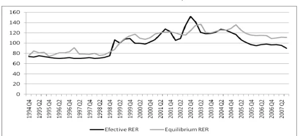
Fig.2 shows the evolution of the effective exchange rate and the equilibrium exchange rate calculate by the model.
11
There, we can observed a significant overvaluation of the rate of exchange during (1994:4 – 1998:4) and (2005:1 – 2007:4). Moreover, during 1994-2004, the real exchange rate shows a marked tendency to depreciate, only slightly inverted during 2005-2007.
Therefore, it is incorrect to state9 that its movements are essentially driven by the appreciation of its equilibrium value. Notwithstanding the latter’s appreciation in the last three years, the appreciation of the actual rate was much greater, thus generating a significant misalignment, which can be estimated to be around 18% in the last quarter of 2007.
3 – Effects of the misalignment
We are now going to look at the effects of the misalignment in particular onto the Brazilian rate of growth, the current account balance and finally its productive structure10 .
We regress the GDP rate of growth (GGDP) onto a set of variables, among them MIS as a measure of the exchange rate misalignment11:
GGDP = + 1INV + 2 EXPORT + 3 CGOV + 4MIS + ui (8)
Where: INV é the ratio of gross fixed capital formation to GDP (INV/GDP); EXPORT is the rate of growth of exports; CGOV is the rate of growth of government consumption in relation to GDP and DES is the rate of exchange misalignment, e.g., the ratio of misalignment to the exchange rate equilibrium value. These are quarterly data obtained from IPEA.
12
To correct for possible bias or inconsistency in the estimation through ordinary last square (OLS), equation (8) above is now estimated by the method of Instrumental Variables, and results are reported in Table 4 below.
Table 4 about here
As is clear, the parameters in the IV ad OLS models show the signs predicted by the theory of demand-driven growth12 and their values are significant. As for the effects of the variable for misalignment on the growth rate, the sign is negative, in other words, the higher the rate of misalignment the slower is economic growth, a result consistent with existing evidence in the literature (e.g. Frenkel, 2004; Razin and Collins, 1997).
We now look at the dependence of growth performance on an exchange rate over-evaluation (OVERVAL). Equation (8) is estimated once again replacing the series of MIS with OVERVAL. To construct the latter we will be using only the negative values of the former, and get the results in Table 5.
Table 5 about here
On the basis of both OLS and IV estimations, the coefficient of the overvaluation variable is negative and significant. Moreover, it is greater that in the case of misalignment, this indicating that economic growth is more negatively affected by misalignment associated with overevaluation.
13
Figure 3 about here
This would be the shortcoming of a “scarcity of domestic savings” to finance productive investment. It would be such scarcity driving the recent valorization of the rate of exchange, hence it would be the consequence of the valorization of its equilibrium level, instead of the misalignment (Pastore et als, 2008). On the contrary, our econometric tests show the existence of a significant misalignment since the second quarter of 2005. Thus, the behavior of the Brazilian current account balance cannot be uniquely attributed to domestic savings scarcity.
It is worth noticing that the reduction of the current account balance coincides temporally with the emergence of an overvaluation of the real exchange rate. There is an inverse relationship between exchange overevaluation and the current account balance as a ratio of GDP between 2004 and 2007. This is to say that the observed reduction of the current account balance in that period is associated with a clear-cut increase in the rate of exchange overevaluation.
Moreover, taking as a reference the behavior of the growth rate of export and import since 2006, one can ascertain the existence of a medium run tendency to the trade balance, and therefore of a tendency to a progressive deterioration of the balance of the current account. Since then, the growth rate of import is higher that the growth rate of export, thus slowly eating up the trade balance surplus. If such a tendency were to persiste in the next years, we would be back with the old problem of the external constraint, which was partly responsible for the slow growth of the last 20 years.
14
technology sectors in total exports13. As the high and medium technology products have a higher demand elasticity with respect to income, that reduction in their share of total exports, is bound to lead eventually to a reduction of the income elasticity of the demand for Brazilian exports, thus to an aggravation of the present disequilibrium between the rates of growth of export and import.
Table 6 shows the trade balance data of manufacturing industry in Brazil.
Table 6 about here
It can be seen from Table 6 that the most important sector in the generation of trade surplus for Brazil, considering the technological intensity, is the low intensity, followed by medium-low segment, but with a considerably lower result. The IEDI (2009) points out that the sub-sectors of food, beverages and tobacco, alone accounted for 78.8% of the balance generated by the sector in 2008.
For the next sector deficits, high and medium high-technology, the two have been running trade deficits or very close to zero for all analyzed periods. Noteworthy is the amount of the deficit generated by the segment of medium-intensity (US$ -30.2 billion in 2008). Finally, the high tech segment in 2008, reached a deficit of US$ -21.7 billion.
As regards the trade surplus generated by the manufacturing industry, this, which showed a clear upward trend between 2003 and 2005, as shown in Table 6, in 2006 this trend was reversed, and in 2008 the deficit of sector was US$ 7.2 billion.
15
maintain that the overappreciation of the exchange rate is driving the Brazilian economy toward deindustrialization, there is strong evidence that the present pace of exchange rate is negatively affecting its industrial structure.
Our reading of the present situation is further supported by the inspection and interpretation of certain indicators that appear in Fig. 5.
Comparing the first quarter of 2004 with the same of 2008, one can detect a remarkable reduction in the industry share in GDP, from 29,4% down to 26,2%. Similarly, the transformation industry also has reduced its share, falling from 18,9% to 15,2%.
Figure 5 about here
It will be argued in the next section that the elimination of the exchange misalignment would have relevant impacts upon the rate of interest. Then, the problem of the exchange rate is strongly associated with the modus operandi of the monetary policy in the country.
4 – At the roots of the loss of efficacy of monetary policy in Brazil14.
16
inflation, something that further increases the level of interest rate required to ensure the convergence of inflation to its long run target values. We have seen this already in action in the previous section.
To support such interpretation, we will now estimate the relevance of the exchange rate in the reaction function of the Central Bank, using an Autoregressive Vector (VAR) model. To do this we have to identify the causality relation between the principal variables that enter the determination of the interest rate. These variables will be: interest rate (Selic) set by the Central Bank; the Extended Consumer Price Index (IPCA), calculated by the Brazilian Institute of Geography and Statistics (IBGE); the exchange rate Real/US Dollar15 as results from Institute of Applied Economics (IPEADATA); the inflation expectations that are monitored in the Boletim Focus of the Central Bank; finally the montly value of the degree of capacity utilization from IPEADATA.
In this was we will be able to estimate the dynamics of the determination of the Selic rate in the period July 2001 to April 2008, in particular trying to quantify the relevance of exchange rate for monetary policy. Our choice of time period was determined by the aim of discarding the earlier two years of inflation targets regime, and analysing the behaviour during a time interval characterised by an already consolidated regime with monetary anchor16.
4.1 The determination of the SELIC rate as a dynamic process
The VAR methodology used hereafter, is utilized also by the Central Bank to estimate the expectations of IPCA and industrial production. It can also be used as a decision support in monetary policy17.
17
and trend, to avoid problems of spurious results leading to incorrect interpretations. The ADF test was once again implemented, as it permits to incorporate extra lagged terms of the dependent variable as a way to eliminate autocorrelation in residuals.
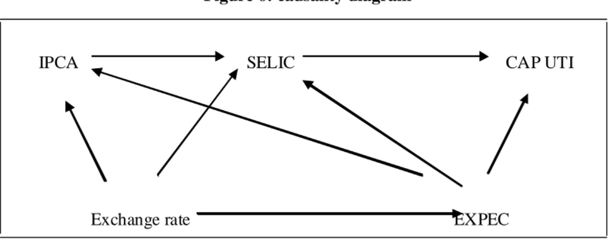
Based on the econometrics tests, certain inferences can be made about the dynamic interaction between variables. The diagram of causality between variables, reported below, is instructive as it synthetizes all significant relations derived with Granger causality test18.
Its analysis yields the following results. The Selic is caused by the exchange rate variable, IPCA and the inflation expectations; the IPCA by inflation expectations and exchange rate; expectations on their turn are caused by exchange rate and this latter is exogenously determined. Finally, the level of capacity utilization is caused by the IPCA, expectations and SELIC. Fig 6 shows such relationships.
Figure 6 about here
In Fig. 6 we see that the exchange rate causes the Selic, both directly, and indirectly through expectations and IPCA. Through its impact on the Selic, the rate of exchange also causes the level of capacity utilization. In fact, the exchange rate is treated here as an exogenous variable, being the principal determinant of all other variables. This is further confirmed by the test for endogeneity. As it can be easily ascertained, the level of capacity utilization, the Selic, the IPCA, and expectations, follow, in this order, the exchange rate in terms of increasing degrees of exogeneity.19
18
From the variance decomposition it can be ascertained that, with a 6-month lag, approximately 47,51% of the changes in expectations taking place are due to movements in the exchange rate. In the same way, an change in the rate of exchange and inflation expectations explain, with a 5 and 2-month lag, about the 37,7% and the 37,54% respectively of the change in IPCA. Moreover, with a 12-month lag, about 22,6% of the change in the SELIC rate can be explained by the change in the exchange rate. Finally, with a 12-month lag, some 11,81% of the change in the capacity utilization rate can be explained by a change in the Selic.
4.2 Interpreting econometric results
The high share of controlled prices in the composition of the IPCA and the relevance of the rate of exchange in the determination of the Selic, both directly and indirectly through expectations and the IPCA itself, dictate a perverse pace of monetary policy. This happens partly due to certain amplifying effect that high portion of controlled prices has onto interest rates. Actually this fact has as a shortcoming that any exchange rate variation exerts greater effects onto prices and finally the interest rate than otherwise.
The dynamics of the determination of the Selic, as shown by our econometric exercises, indicate that the action of interest rates over the output gap does not comply with the logic of a traditional Phillips curve. In this logic, in fact, a rise in nominal, and real, interest rates would cause a reduction in output levels, thus forcing a reduction in the inflation rate.
19
consequence of the fact that the former, while causing changes in the rate of capacity utilization, has no perceivable effect upon the exchange rate or the inflation rate. Put differently, the changes in exchange rate values do cause changes in the rate of inflation and the interest rates, so that monetary policy ends up having to react to a cost inflation pressure, but has no little or no effect as a measure to control the Brazilian inflation.
20
5 – The Determination of interest and exchange rates in Brazil: the perverse interaction of monetary and exchange rate policy.
In the last two sections we saw that Brazilian economy in period 2004-2008 was characterized by a significant exchange rate over-valuation that had negative effects over GDP growth and was caused, among other variables, by the high level of short term interest rates prevailing in Brazil as compared to the ones prevailing in the rest of the world. We also saw that the high level of short term interest rate in Brazil is a direct consequence of a sort of “excess of conservatism” of monetary authorities in Brazil whon react to negative supply shocks originated in the external sector of the economy by means of an increase in the short term interest rate.
We will now see how these peaces fits together; i.e, how exchange rate policy and monetary policy interact one with another in order to produce a perverse combination of a high interest rate and a low exchange rate.
Although monetary authorities in Brazil intervene in exchange rate market, exchange rate regime in Brazil can be considered a (dirty) floating since there is no commitment of Central Bank with a pre determined exchange rate level. Since the majority of capital controls were removed in Brazil in the beginning of the 1990´s, we can suppose that a situation of near perferct capital mobility prevails in Brazilian economy. This means that the short term dynamics of nominal exchange rate can be explained by means of the uncovered interest rate parity as show by equation (10).
i = i* + (Ee /E) – 1 (10)
21
From the estimation of reaction function of the Central Bank we can say that short-term nominal interest rate is deshort-termined by:
i = f(E, ….) , f ´> 0 (11)
Combining equations (10) and (11) we can determine shot term interest rate and nominal exchange rate, as shown by figure 7.
Figure 7 about here
Consider now an exogenous increase in price level of commodities – for example, caused by speculation in commodity markets. This will be equivalent to a negative supply shock, causing an immediate increase in dometic rate of inflation. According to the econometric model shown in section 4, monetary authorities in Brazil will react to such an event by means of an increase in the short-term interest rate, displacing the RF curve to the left (figure 8). As a consequence of interest rate increase, nominal exchange rate will fall (appreciation), increasing the over-valuation of real exchange rate.
Figure 8 about here From figure 8 we can see that the combination of a (dirty) floating exchange rate system with a rigid inflation targeting regime can produce a perverse combination of high short-term interest rate and over-valued exchange rate in face of negative supply shocks. The elimination of the “high interest rate-low exchange rate trap” is a necessary condition for the relaxation of macroeconomic constraints to long-term growth of Brazilian economy. In the next section we will present some policy proposals to solve this macroeconomic problem. 6 – Policy Proposals
22
rate, while at the same time it has to alter fundamentally the modus operandi of the monetary policy, allowing for a temporary rise in the inflation rate. This latter is necessary to make possible an adjustment in the real exchange rate, without initializing a process of rising interest rates.
A controlled exchange rate depreciation has to be realized through purchases of international reserves by the Central Bank. Such operations have to aim not just at an increase in the international reserves, but at the gradual elimination of the exchange misalignment. In other words, the Central Bank has to operate having implicit targets as to the nominal rate of exchange.
To reach such targets without restricting the BCB freedom to fix the basic rate of interest, it will be necessary to to introduce a system of control over the outflow of short term capital. In fact, from the moment economic agents will perceive that the monetary authority is pursuing an implicit exchange rate target, implying a gradual depreciation of exchange rate, there will be a capital flight from the country. This outflow will be further reinforced by the reduction in domestic interest rates, following the change in the approach to monetary policy.
Recalling the international experience of capital controls, in particular on the basis of the lessons learned during the exchange rate crisis of Malaysia (1997-8), controls on outflows will have to be of an administrative and all encompassing character, so as to to be bypassed. A temporary prohibition to capital exit is not to be discarded as a measure in the initial phase of implementation of this new macroeconomic policy model.
23
the interest rate hike that would follow the elimination of the exchange misalignment, but also to reduce the fiscal costs of the exchange policy.
On the other hand, the switch in monetary policy has to go together with the substitution of actual inflation targeting regime (ITR, hereafter) for a “double mandate regime” (DMR, hereafter) where Brazilian monetary authorities must pursue two objectives of monetary policy; that is: output stabilization and inflation control. Although advocates of ITR stress that both functions can be performed by this framework of monetary policy (see Bernanke et al, 1999), we do not share this optimistic view for a variety of reasons. First of all, ITR is based on New Consensus on Macroeconomics (Arestis and Saswyer, 2006a, 2006b) that considers output to be supply constrained in the long-run. As we have saw in section 2 of this paper, there are a lot of empirical evidences showing that growth is demand-led in Brazilian economy. Second, ITR take for granted that inflation acceleration is always and elsewhere the result of a situation of excess demand. But this is certainly not the case for Brazilian economy, where inflation responds strongly to variations in nominal exchange rate rather than to variations in capacity utilization. To stabilize inflation in Brazil it is necessary to reduce the level of price indexation to exchange rates, what can be done by a simple change of contracts of public services, forcing controlled prices to be indexed by IPCA (General Consumer Price Index) rather than by IGP-M (General Level of Market Prices), which is an index that, by construction, follow the behaviour of nominal exchange rate. As a complementary device for inflation control it is necessary for Brazilian Treasury to get rid off indexed public bonds, the so-called Letras Financeiras do Tesouro, that are also responsible for a low effect of interest rate changes over aggregate demand.
24
available, we can deduce that these rates of inflation are not prejudicial to economic growth in emerging economies (see Sarel, 1996).
7 - Final Remarks.
We have argued that the Brazilian economy has recently gone through a process of accelerated growth, driven both by export growth and by gross fixed capital formation. Although this growth pace is much more robust than the one experienced in the 1990, one can ascertain the existence of macroeconomic constraints to its continuity in the long run. These constraints can lead to a lasting reduction of the economy’s growth rate, the first constraint is in the exchange rate disequilibrium that set in since 2005. This misalignment exerts negative effects upon output growth and has generated a reduction in the current account balance, thus threatening external equilibrium. Moreover, such misalagnimnet may be fostering a concentration of the production structure in those sectors with low added value and/or with low technological content. Such concentration can only be harmful to the long run growth as it induces a reduction in income elasticity of Brazilian exports.
The second constraint lies in the modus operandi of monetary policy. We maintain that the Central Bank has an “excessive care” with the inflation rate, increasing the basic rate of interest on the basis of the inflationary pressures that are generated by changes in nominal exchange rate. Such dynamics brings about the inefficacy of the monetary policy while being one of the causes of the high interest rates in the economy.
25 References
Arestis, P.,Sawyer, M. 2006a. The nature and role of monetary policy when money is endogenous, Cambridge Journal of Economics, 30, 847-860
___________________ 2006b. Interest rates and the real economy, in: c. Gnos, L.P. Rochon (eds.). Post Keynesian Principles of Economic Policy, Aldershot, Edward Elgar
Associação Keynesiana Brasileira.2008. ‘Dossiê da Crise’. Porto Alegre, Nevembro,
http://www.ppge.ufrgs.br/akb
Montiel, P. ; Hinkle, L. 1999. Exchange Rate Misalignment: concepts and measurement for developing countries, Oxford, A World Bank Research Publication.
Banco Central do Brasil 2008. Economia e Finanças: séries temporais,
Easterly, W. 2001. The lost decades: developing countries’ stagnation in spite of policy reform 1980–1998, Journal of Economic Growth, vol. 6, no. 2, 135–57
Edwards, S. 1989. Real Exchange Rates, Devaluation, and Adjustment: Exchange Rate Policy in Developing Countries, Cambridge, MA, MIT Press.
International Monetary Fund FMI. 2007. World Economic Outlook, Washington.
FUNCEX. Fundação de Estudos do Coméercio Exterior. Disponível em < http://www.funcex.com.br/>
Gala, P. 2008. Real Exchange rate levels and economic development: theoretical analysis and econometric evidence. Cambridge Journal of Economics, 32.
Harrod, R. 1939. An Essay in Dynamic Theory, The Economic Journal, vol. 49.
Hinkle, L.E.; Montiel, P.J. 1999. Exchange Rate Misalignment: Concepts and Measurement for developing countries, A World Bank Research Publication, Oxford University Press. IBGE. INSTITUTO BRASILEIRO DE GEOGRAFIA E ESTATÍSTICA, 2008.
IEDI - INSTITUTO DE ESTUDOS PARA O DESENVOLVIMENTO INDUSTRIAL. “Os resultados de 2008 e os Primeiros impactos da crise sobre o comércio exterior brasileiro”, (2009)
IPEA. 2008. Indicadores IPEA, Downloadable at <http://www.ipeadata.gov.br.htm>,.
Ledesma, M.L. 2002. Accumulation, Innovation and Catching-up: an extended cumulative growth model, Cambridge Journal of Economics, Vol. 26, n.2.
Libanio, G. 2009. Aggregate demand and the endogeneity of the natural rate of growth: evidence from Latin American Countries. Cambridge Journal of Economics, 33.
Lima, G.T; Araujo, R. (2007). A structural economic dynamics approach to balance-of-payments-constrained growth. Cambridge Journal of Economics, 31.
Montiel, P. 1999. The Long-Run Equilibrium Real Exchange Rate: conceptual issues and empirical research, in: Hinckle, L.E.; Montiel, P.J. (Eds.) Exchange Rate Misalignment: Concepts and Measurement for developing countries, A World Bank Research Publication, Oxford University Press.
26
O Globo. “Inflação no segundo plano”. 19/12/2008, p.31.
Oreiro, J.L; Paula, L.F; Jonas, G; Quevedo, R. 2008. “Por que o custo do capital no Brasil é tão alto?”, Mimeo.
Pastore, A.C; Pinotti, M.C; Almeida, L.P 2008. Câmbio e Crescimento: o que podemos aprender?, in: Barros, O.; Giambiagi, F. (Eds.). Brasil Globalizado, Campus, Rio de Janeiro. Razin, O.; Collins, S. 1997. Real Exchange Rate Misalignment and Growth, in Razin A. , Sadka, E. (Eds.). International Economic Integration: Public Economics Perspectives, Cambridge University Press, also at NBER Working Paper, n.6147, 1997.
Sarel, M. 1996. Nonlinear effects of inflation on economic growth, IMF Staff Papers 43, p. 199–215.
Thirwall, A. 2002. The Nature of Economic Growth, Aldershot, Edward Elgar.
Figure 1 - GDP, Exports and Gross Fixed Capital Formation (% change p.y)
Source: IPEADATA. Author´s elaboration.
Table 1 – Estimated Values of the NGR Using Okun and Thirwall Equations
METHOD INTERCEPT ANGULAR
COEFF
DW R2 Aj. NGR
Okun’s Equation (1)
RR
1,61 -2,70***
2,32 0,11 0,60
(0,99) (3,49)
Thirwall’s Equation (2)
OLS
0,59*** -0,053***
1,89 0,15
0,59
(2,99) (4,12)
27
Table 2. Estimation of the natural rate in Okun’s and Thirwall’s equations with a dummy variable
Method Intercept Dummy Coefficient
Angular Coefficiente
DW R2
Aj.
NRG (g<gn)
NRG (g>gn)
Equation (4) OLS -0,84*** 2,85*** 0,03*** 2,28 0,61 -0,84 2,01
(-4,40) (10,40) (-3,35 )
Equation (4) MA PWER -0,26* 1,56*** 0,011** 1,82 0,54 -0,26 1,3
(-1,66) (10,26) (-2,14)
Note: *** significant at 1%; ** signiificant at 5%; * signiificant at 10%. PWER is the Prais-Wisten method to deal with autocorrelation issues. DW is the Durbin-Watson value for first order autocorrelation; R2 Aj. is the adjusted value of R2; NGR natural growth rate; e MA is a regression equation using quarterly moving averages.
Table 3 – OLS estimation
statistics Variables
C OPEN INTDIF TAGDP TOT FORP GC
Coefficient 202,84 1,754 -0,219 -4,795 -1,433 -0.070 -0,0003
standard desviation 26,661 0,510 0,112 0,978 0,229 0.009 0,0001
T statistics 7,608 3,441 -1,95 -4,902 -6,264 7.927 -4,050
P-valor 0,000 0,001 0,058 0,000 0,000 0.000 0,0002
R2 0,9311 Adjusted R2 0,9219 F-test 101,346 probability (0,000) Durbin Watson 1,8224
28
Figure 2 – Actual and expected values of the real exchange rate ( indexed – average value of 2000=100)
Source: Auhors´s own elaboration.
Table 4 – Growth regression
Variable OLS IV
INV 0.197733
0.071899 (2.750579)**
0.11711 0.05921 (1.977826)**
EXPORT 0.266595
0.056591 (4.710873)*
0.233294 0.055152 (4.230035)*
CGO 0.010415
0.002655 (3.922720)*
0.008911 0.002598 (3.430203)**
MIS -0.116802
0.067390 (-1.732255)***
-0.110111 0.068325 (-1.628097)***
GDP(-1) 0.068593
0.036474 (1.880627)***
0.069599 0.035365 (1.96801)**
C 0.344253
0.118065 (2.915798)**
0.214945 0.098481 (2.182608)**
R2 0.393741 0.348120
Adjusted R2 0.329245 0.293797
F-statistics 6.104924 6.184924
Prob. (F test) 0.000196 0.000195
Durbin-Watson 2.283926 2.346569
Note: *significant at 1%, ** significant at 5% e *** significant at 10%.
29
Table 5 – growth regression with OVERVAL
Variable OLS IV
INV 0.197733
[0.071899] (2.750579)**
0.211330 [0.07198] (2.936096)**
EXPORT 0.266595
[0.056591] (4.710873)*
0.346081 [0.060676] (5.703727)*
CGO 0.010415
[0.002655] 3.922720*
0.011569 [0.002581] (4.482158)*
OVERVAL -0.116802
[0.067390] (-1.732255)**
-0.244340 [0.131764] (-1.854370)*
GDP(-1) 0.068593
[0.036474] (1.880627)**
0.088049 [0.036154] (2.435355)**
C 0.344253
[0.118065] (2.915798)**
0.350143 [0.118797] (2.947391)*
R2 0.393741 0.520940
Adjusted R2 0.329245 0.459522
F statistics 6.104924 8.481891
Prob. ( F test) 0.000196 0.000017
Durbin-Watson 2.283926 2.385196
Nota: *significant at 1%, ** significant at 5% e *** significant at 10%.
Standart desviation in [ ] and T test in ( )
Figure 3: Dynamcis of the ratio of current account balance to GDP (1994-2008)
-5 -4 -3 -2 -1 0 1 2 3 199 4 199 5 199 6 199 7
1998 1999 2000 2001 2002 200 3 200 4 200 5 200 6 200 7 200 8
30
Table 6 – Trade balance of manufacturing industry in US$ billions
2003 2004 2005 2006 2007 2008
Low technological intensity 19.856 25.197 28.727 31.927 34.761 39.559
Medium-low technological intensity 5.488 8.871 10.258 10.545 9.185 5.118
High-Medium technological intensity -3.376 -2.531 443 -897 -10.344 -30.190
High technological intensity -5.245 -7.484 -8.320 -11.779 -14.824 -21.653
Total manufacturing industry 16.723 24.053 31.107 29.796 18.779 -7.166
Source: IEDI (2009)
Figure 5 – Share of Manufacturing Industry in GDP
31
Figure 6: causality diagram
IPCA SELIC CAP UTI
Exchange rate EXPEC
Figure 7
RF
UIP
E i
32 Figure 8
Footnotes: **
Associate Professor, Departamento de Economia, Universidade de Brasília and Level I Researcher of National Scientific Council (CNPq). E-mail: joreiro@unb.br.
***
Professor, Department of Economics, Università di Siena, Italy. E-mail: punzo@unisi.it. ****
Associate Professor, Department of Economics, Universidade Estadual de Maringá. E-mail: elianedearaujo@gmail.com.
*****
Economist at IPEA/DF. E-mail: gabrielcoelhosqueff@gmail.com. RF0
UIP
E i
E1 E0
i1 i0
33
1The time period of our analysis ends in 2002 due to a methodological change that occurred in the Monthly Employment Survey from 2003, which impeded the extension of econometric tests to the most recent period due to change in the database.
2 Similar results are obtnained by Libanio (2009) who estimated an endogenous natural growth rate of Brazilian economy equal to 6.68 % p.y. In the empirical model that we developed in this section, we arrived at different values for the endogenous natural growth rate from those obtained by Libanio. Indeed, our empirical model suggests that endogenous natural rate of growth can be 5.2% p.y or 8% p.y in boom times, depending on the
specification of the econometric model. In fact, by using a MA model, the estimated value for the endogenous natural rate of growth of the Brazilian economy is considerably reduced. The use of a MA model is an important improvement with the work of Libanio since time series data used in the estimation of the endogenous natural rate of growth is of a quarterly periodicity.
3Ledesma, 2002, estimates a demand driven model for a set of 17 OECD (West Germany, Australia, Áustria, Belgium, Canada, Denmark, USA, Spain, Finland, France, Italia, Holland, Japan, Norway, Portugal, Sweden and UK) in the 1965-1994 period
4
The latter comes from the Pesquisa Mensal do Emprego (PME, monthly Unemployment Survey) of the Instituto Brasileiro de Geografia e Estatística (IBGE). From monthly date we have constructed quarterly data with an arithmetic average over the quarter year The GDP chain index is constructed from the System of National Accounts produced by IBGE (IBGE/SCN). The period under investigation begins with the first quarter of 1980 to end with the last of 2002. The two variables were transformed in rates of changes.
34
6Montiel, 1999, p.221. Among other things, a long run equilibrium implies the absence of all types of speculative bubbles.
7
The methodology follows three steps. In the first step, adapting received economic theory to the actual situation of the economy to be studied, a long run relationship is sought to then be estimated. Its parameters are estimated in the second step using techniques suited for the time series being used. In the last step, the estimated values of the parameters are utilized to compute the long run equilibrium rate of exchange.
8See Ahler and Hinkle 1999
.
9For an example, see Pastore et al, 2008, p.283. 10
For a theoretical account of the effects of over-valuation of real exchange rate over economic growth and some empirical evidence for Latin America and East Asia see Gala (2008). It is important to notice that Gala´s work on real exchange rate and economic growth is not based in the calculation of an exchange rate misalignment, but instead used the index of exchange rate over-valuation developed by Easterly (2001). The calculation of the rate of exchange rate misalignment and its effect over GDP growth of Brazilian economy is an important novelty of the present work.
11where: INV é the ratio of gross fixed capital formation to GDP (INV/GDP); EXPORT is the rate of growth of exports; CGOV is the rate of growth of government consumption in relation to GDP and DES is the rate of exchange misalignment, e.g., the ratio of misalignment to the exchange rate equilibrium value. These are quarterly data obtained from IPEA.
12The lagged rate of growth of GDP (GDP-1) was introduced as an explicatory variable in equation 8 to address the problem of autocorrelation.
13For a theoretical analysis of the relation between strucutural change and economic growth see, among others, Lima and Araujo (2007).
35
15We are taking the average value of the so called commercial rate of exchange.
16A non secondary motivation for our choice is in fact that only since 2001 is data on inflation expectations being collected
17As is the case with the Relatórios de Inflação (Inflation Reports) by the BCB. 18
The ADF test shows that all variables being considered are first difference stationary. With the exepcions of expectations and the exchange rate, showing a lag of 3 and 2 periods, respectively, all other variables have a 1-lag as the best lag structure, according Schwarz criterion. The best phase structure for the model as a whole has 2 lags, as for the time period the LM test (the Lagrange Multiplier Test) does not show significance in terms of serial correlation of residuals.With that lag structure, we applied the Granger causality test, estimated the error variance decomposition and the orden of endogeneity of the variables- by means of the VAR Pairwise Granger Causality. Finally, with the view of checking for the existence of a long run relationship between variables, Johansen cointegration test was applied, from which at least two cointegration vectors at a 5% significance level were identified.