UNIVERSIDADE DE S ˜AO PAULO INSTITUTO DE F´ISICA
Estruturas em larga escala e o
Dark Energy Survey
Hugo Orlando Camacho Chavez
Orientador: Prof. Dr. Marcos Vinicius Borges Teixeira Lima
Disserta¸c˜ao apresentada ao Instituto de F´ısica da Universidade de S˜ao Paulo para a obten¸c˜ao do t´ıtulo de Mestre em Ciˆencias.
Banca Examinadora:
Prof. Dr. Marcos Vinicius Borges Teixeira Lima (IF-USP) Prof. Dr. Luis Raul Weber Abramo (IF-USP)
Prof. Dr. Gast˜ao Bierrenbach Lima Neto (IAG-USP)
!
"
#!
$
!
"
!
" # $% & ' ( " " ) " *+ " , *+ " % - "
" . / % 0" " " 1 2 "3 " 4"
5 # . "
( " . 6 " 7 " 7 8 "
Abstract
Modern wide-area multi-color deep galaxy redshift surveys provide a powerful tool to probe cosmological models. Yet they bring new practical and theoretical challenges in order to exploit the information contained in their data. This dissertation reviews the theoretical interpretation of clustering of galaxies and shear/convergence weak lensing effects by the large scale structure of the Universe in the context of FLRW cosmological models. This interpretation is general in the sense that the effects of the spatial curvature are properly taken into account, thus holding for FLRW Universes with arbitrary content of matter and dark energy. In this context, we consider two-point statistics both in con-figuration and harmonic spaces, providing general formulae for the two-point correlation function in real and redshift space. We further include wide angle effects and consider the proper distant observer approximation.
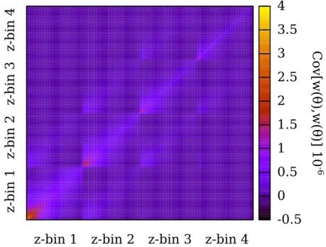
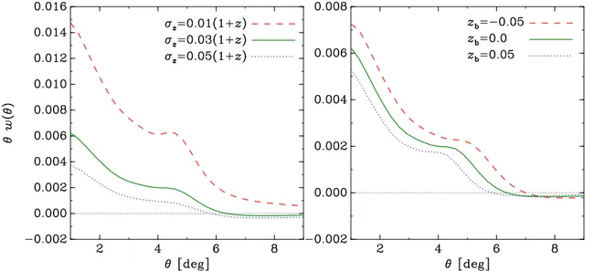
One main characteristic of photometric galaxy surveys is that they will gain in area and depth, in exchange for a poorer determination of radial positions. In this context splitting the data into redshift bins and using the angular correlation function (ACF)w(θ) and the angular power spectrum (APS)Cℓconstitutes a standard approach to extract cosmological information. This dissertation also addresses the problem of constraining cosmological parameters using Bayesian inference techniques from measurements of the ACF and the APS on large scales. Different computational approaches are discussed to accomplish this goal and a detailed model for the ACF at large scales is presented including all relevant effects, namely nonlinear gravitational clustering, bias, redshift-space distortions and photo-z uncertainties.
Resumo
Experimentos modernos com observa¸c˜oes das posi¸c˜oes e redshifts de gal´axias em grandes ´areas do c´eu representam uma poderosa ferramenta para a investiga¸c˜ao de modelos cos-mol´ogicos. Entretanto, estas observa¸c˜oes trazem consigo novos desafios pr´aticos e te´oricos para a extra¸c˜ao da informa¸c˜ao contida nos dados. Esta disserta¸c˜ao faz uma revis˜ao da in-terpreta¸c˜ao te´orica da aglomera¸c˜ao de gal´axias e dos efeitos de lenteamento gravitacional fraco por estruturas em largas escalas no Universo, no contexto de modelos cosmol´ogicos FLRW. Esta interpreta¸c˜ao ´e geral, na medida em que os efeitos da curvatura espacial s˜ao apropriadamente considerados, sendo portanto verdadeiros para Universos FLRW com conte´udos artibr´arios de mat´eria e energia escura. Neste contexto, consideramos a estat´ıstica de dois pontos no espa¸co de configura¸c˜oes e no espa¸co harmˆonico, obtendo f´ormulas gerais para a fun¸c˜ao de correla¸c˜ao de dois pontos no espa¸co real e no espa¸co de redshifts. Inclu´ımos ainda efeitos de grandes ˆangulos e consideramos a aproxima¸c˜ao de observador distante de forma apropriada.
Uma caracter´ıstica importante de levantamentos fotom´etricos de galaxias ´e a de que eles v˜ao ganhar em ´area e profundidade, em troca de uma pior determina¸c˜ao das posi¸c˜oes radiais. Neste contexto, uma t´ecnica padr˜ao para extra¸c˜ao de informa¸c˜ao cosmol´ogica dos dados consiste em dividir as gal´axias em bins de redshift, de forma a assim usar a fun¸c˜ao de correla¸c˜ao angular (ACF) w(θ) e o espectro de potˆencias angular (APS) Cℓ. Nesta disserta¸c˜ao tamb´em tratamos o problema de vincular parˆametros cosmol´ogicos usando t´ecnicas de inferˆencia estat´ıstica Bayesiana a partir das medidas da ACF e do APS em grandes escalas. Diferentes t´ecnicas computacionais s˜ao discutidas e um modelo detalhado para a ACF em grandes escalas ´e apresentado, incluindo todos os efeitos relevantes, como n˜ao-linearidades gravitacionais, o bias, distors˜oes no espa¸co de redshift, e incertezas nas estimativas de redshifts (photo-zs).
Acknowledgments
First and foremost I would like to thank my advisor Marcos Lima, for all his help, support, guidance and constant encouragement without which this truly would not have been possible. I would also like to thank everyone in the Cosmology group at Departamento de F´ısica Matem´atica da Universidade de S˜ao Paulo (DFMA/IF/USP), for providing the best work environment and for the valuable discussions on the seminars and classes, in particular Michel Aguena for his constant and enjoyable collaboration and friendship and for useful comments and discussions during the preparation of this work, and also Lucas Secco, Leandro Beraldo, Henrique Xavier, Ricardo Landim, Leonardo Duarte, Carolina Queiroz, Andr´e Alencar, Arthur Loureiro, Leila Graef, Riis Bachega and Lucas Olivari. I profited profusely from our countless discussions.
I would like to thank all the DES-Brazil team for useful discussions during the prepa-ration of this work. I also like to express my appreciation to the co-referees of my thesis, in particular to Raul Abramo, for his valuable comments and discussions.
I am very grateful to Leonardo Casta˜neda for introducing me to Cosmology and for his valuable friendship and to all my friends of the Gravitation and Cosmology group at Universidad Nacional de Colombia, in particular to my old friend Sergio Rodriguez for his constant encouragement and valuable friendship through all this years.
I would like to thank to all my family for their constant support and encouragement, without them none of this would be possible, and to my friends Oscar Lopez (RIP), Diego Fabra, Yuber P´erez, Antonio Sanchez, Faiber Alonso, Cristian Duitama, Leonardo Gil, Jonathan Mancilla, Ramiro Beltran, Andr´es Manrique, Maria Fernanda Gonzalez and all those outside of this list that would otherwise be very long. I am very grateful for all your teachings.
Contents
1 Introduction 1
1.1 Standard model of cosmology . . . 3
1.2 Cosmological perturbation theory . . . 8
1.2.1 Linear growth of structures . . . 9
1.2.2 Nonlinear evolution . . . 11
1.3 The Dark Energy Survey . . . 18
1.4 LSS cosmological observables . . . 18
1.4.1 Three and two-dimensional galaxy clustering . . . 18
1.4.2 Weak gravitational lensing . . . 20
2 Two-point statistics in the Universe 25 2.1 Configuration space . . . 27
2.1.1 Correlation function and power spectrum . . . 27
2.1.2 Estimation techniques in configuration space . . . 31
2.1.3 Comparison of different estimators . . . 37
2.2 Harmonic space . . . 37
2.2.1 Angular power spectrum . . . 37
2.2.2 Simple estimator for the angular power spectra . . . 40
3 Statistical inference 43 3.1 Bayes’ Theorem . . . 44
3.2 Bayesian parameter inference . . . 46
3.3 MCMC techniques for model parameter Bayesian inference . . . 47
3.3.1 Metropolis-Hastings sampling . . . 48
3.3.2 Affine-invariant ensemble MCMC . . . 48
4 Results 53 4.1 Two-point statistics in configuration space . . . 54
4.1.1 Galaxy two-point correlation function in FLRW Universes . . . 55
4.1.2 Angular two-point correlation function of galaxies . . . 64
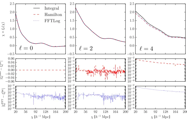
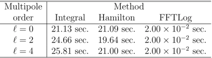
4.1.3 Computing the multipoles of the two-point correlation function . . 71
4.1.4 SDSS-III DR8 photometric luminous galaxies ACF . . . 75
4.1.5 BCC-Aardvark-v1.0 red galaxies ACF. . . 87
4.2 Two-point statistics in harmonic space . . . 96
4.2.1 The onion simulation maps . . . 97
4.2.2 Angular power spectra measurements and modeling . . . 97
4.2.3 Simple cosmological analysis of APSs from Onion simulations . . . 98
Appendices 109
A Cosmological perturbations 109
A.1 Background Geometry . . . 109
A.2 Perturbation theory and the gauge problem . . . 110
A.2.1 Taylor expansion of a tensor field . . . 111
A.2.2 Gauge transformations and gauge invariance . . . 112
A.3 First order perturbations . . . 114
A.3.1 Scalar–vector–tensor decomposition . . . 114
A.3.2 Metric perturbations . . . 115
A.3.3 First order scalar perturbations . . . 116
A.3.4 Matter–energy perturbations . . . 118
A.3.5 First order Einstein field equations . . . 119
B Scalar harmonic modes in the Universe 123 B.1 Harmonic decomposition of a scalar field . . . 130
C Linear redshift space distortions in the Universe 133 C.1 Redshift . . . 134
C.2 Redshift–space radial distance and coordinate . . . 134
C.3 Redshift–space distorted fluctuations of matter . . . 136
C.4 Redshift–space distortion operator . . . 139
D Deflection of light rays by LSS in the Universe 141 D.1 Geometric optics approximation . . . 141
D.2 Background null geodesics . . . 143
D.3 First order perturbed null geodesics and deflection angle . . . 144
E FFTLog method 149 E.1 Discrete Fourier transform . . . 149
E.2 Discrete Hankel transform and FFTLog method . . . 150
E.3 Mellin transform of Bessel functions of the first kind . . . 152
Chapter 1
Introduction
One of the main challenges in modern cosmology is the study of the large-scale structure of the observable Universe, its relation to astrophysical phenomena such as galaxy formation on the one hand and to the Universe evolution on large scales on the other hand. In particular, the latter may help shed light on yet unknown fundamental physics, which seems necessary to explain recent observations.
In recent years cosmology entered what can be called a “golden age”, due to two fundamental reasons: (a) our knowledge about the Universe appears to be consolidating along with all observational data that seem to converge consistently into a standard cos-mological model (a concordance model) and (b) on top of this consolidation, cosmology faces many theoretical and practical challenges. The theoretical challenges are mostly related to the physical nature of the constituents of the concordance model, as for exam-ple, the nature of dark matter, of dark energy or cosmic acceleration, and of inflation. The observational challenges are mainly related with the variety of observational probes proposed, their proper interpretation and the necessity of dealing with large amounts of data that are expected from current and upcoming observations.
The relation between redshift and physical distances depends on the expansion rate and the spatial geometry of Universe. In addition, the expansion rate slows down the gravi-tational evolution of cosmic structure. Therefore, by measuring the distances and growth of cosmic structures, one can constrain the properties of dark energy.
This dissertation is organized as follows. This first chapter sets the foundations of the work, as the standard cosmological model is reviewed. We do not intend to provide an exhaustively complete revision, but only the most fundamental aspects that will be necessary later. Our treatment is based on the original treatments of textbooks [2, 3, 4] and the Carg`ese lectures of 1998 [5], which we recommend for further discussions. In section 1.2 we consider perturbations around the background expansion following the same textbooks and original developments presented on [6]. In section 1.3 we briefly discuss the Dark Energy Survey. The chapter ends in section 1.4, where two of the four observational probes considered in the DETF are interpreted in the context of FLRW Universes. More precisely, the galaxy number fluctuation field is presented as the basic concept for understanding clustering and the cosmic shear and convergence fields are also presented as analogs for the weak lensing phenomena by LSS in the Universe. Our discussions follow the original works [7, 8] and [9] in the galaxy clustering section and the review articles [10, 11] as well as §7.1 of [3] for the weak lensing section, which we recommend for further details. Some further theoretical details and computations are also left for the appendices.
In chapter 2, the two-point statistics of these fields is considered and its relation to the total matter power spectrum today is derived. This relation is the basic tool to properly compare cosmological observations with theoretical models.
In chapter 3, Bayesian statistical inference methods are reviewed as the basic tool to constrain cosmological parameters from observations. In this context the sampling problem is depicted and the widely used Markov Chain Monte Carlo (MCMC) methods are presented as a reliable solution. The recent method of affine-invariant MCMC is also discussed as a powerful alternative for solving efficiently the problems of sampling degener-ate probability distribution functions with the possibility of using parallel computational resources.
In chapter 4, the main results of the present dissertation are presented. Initially a general formula for the two-point correlation function of galaxies in redshift space is pre-sented, accounting for wide angle effects, arbitrary redshifts and spatial curvature. From them, the distant observer approximation is considered. Then, a model for the angu-lar correlation function of galaxies at angu-large scales is presented, accounting for nonlinear gravitational clustering, bias, redshift space distortions and photo-z uncertainties. An analysis of the large-scale angular correlation function is presented for the CMASS lumi-nous galaxies (LGs), a photometric-redshift catalog based on the Data Release 8 (DR8) of the Sloan Digital Sky Survey-III, showing that the ACF can be efficiently applied to constrain cosmology in future photometric galaxy surveys. The results of this work have been published in [12]. Another analysis of the ACF on large scales but for a simulated catalog of the DES collaboration is also presented. We end the chapter with an analysis of simple measurements of the APS from galaxy positions on the Onion Universe Simu-lation [13]. Measurements of the auto-correlation of the convergence field and the cross correlation of convergence and galaxy positions are also considered but are not used on the cosmological analysis.
1.1 Standard model of cosmology 3
1.1
Standard model of cosmology
The Universe is observed to be isotropic about us to a high degree of confidence, once we (a) average over large enough scales, considerably larger than the typical scales of clusters of galaxies, and (b) allow for an observer peculiar velocity relative to the average motion of matter in the Universe. In practice, this velocity is treated as relative to the microwave background radiation1. In other words, on cosmologically observable scales, there is no
particular direction that can be stated to be the center of the Universe. One ends up with two possibilities: (a) either the Universe is spatially homogeneous, and as an specific observer we are on a typical place as the Universe is isotropic for any typical observer, or (b) the Universe is spatially inhomogeneous, and we are near a distinguished place with respect to which the Universe looks isotropic. The common choice of the modern scientific community is the former one. It is commonly interpreted as a Copernican principle, i.e., the assumption that we are not at a privileged position in the Universe [14, 2]. The Copernican principle along with the observed isotropy are sufficient conditions for the global spatial homogeneity of the Universe [2].
The modern standard cosmological model then assumes that the Universe is spatially homogeneous and isotropic. Combined, these two assumptions are commonly known as the cosmological principle. Spatial homogeneity imply the existence of a one-parameter family of space-like hypersurfaces Σt, foliating the spacetime, in which the Copernican principle is valid and therefore every point is equivalent. On the other hand, spatial isotropy imply the existence of a congruence of time-like worldlines with tangent vector
ua defining the four-velocity of the so-calledisotropic observers, such that it is impossible to construct a preferred tangent vector perpendicular toua 2. Combining both conditions
imply that the four-velocity of isotropic observers ua and the homogeneity hypersurfaces Σt should be perpendicular, otherwise the Universe should have a privileged spatial di-rection violating isotropy. Then, viewed as three-dimensional subspaces, the Σt surfaces are maximally symmetric, and consequently are spaces of constant curvature [14,2]. The isotropic observers acquire the property that for each instant of proper time, they ob-serve a maximally symmetric 3D space, which is why they are also called fundamental observers.
Therefore, one can define a coordinate time t, the cosmic time, as the proper time measured by the fundamental observers, dt = dxau
a in terms of which the metric of spacetime can be written as
gab=uaub+bγab(t), (1.1) where for each value oft,bγab(t) determines the metric of the constant time hypersurfaces Σt. Since this hypersurfaces should be of constant curvature for each cosmic time instant, one can choose comoving spatial coordinates (xi) to separate the time dependence and write the spacetime metric tensor as
¯
g=−dt⊗dt+a 2(t)γ
ijdxi⊗dxj, (1.2)
where the function a(t), giving the time evolution of the hypersurfaces Σt, is the cosmic
scale factor, determining how physical spatial scales change with time and relate to the comoving scales. The spatial metric of components γij in comoving coordinates defines
1
See AppendixCfor a discussion of this point.
2
generic 3D spaces of constant curvature. A spacetime metric with the form of (1.2) and the above characteristics is known as a Robertson-Walker metric (RW).
For the purposes of this work it is useful to introduce the conformal time η by the relation adη = dt, in terms of which the RW metric (1.2) reads
¯ g=a
2(η)
−dη⊗dη+γijdxi⊗dxj . (1.3) For the constant time hypersurfaces one can always choose spherical coordinates xi = (χ, θ, ϕ), where χ is a radial coordinate and (θ, ϕ) are the usual polar and azimuthal angles of spherical coordinates on the unit sphere S2. During this work χis chosen to be
adimensional for the spatially non-flat cases. The components of the spatial metric for this coordinates choice are given in the (comoving) spatial line element
dℓ2 =γijdxidxj =
−K−1dχ2+ sinh2(χ)dΩ2 K <0,
dχ2+χ2dΩ2 K = 0, K−1dχ2+ sin2(χ)dΩ2 K >0;
(1.4)
where χ ∈ [0,∞) for K ≤ 0, χ ∈ [0, π] for K > 0 and θ ∈ [0, π] and ϕ ∈ [0,2π) for all cases in order to cover the spacetime. This choice of coordinates is particularly useful for our purposes because it leaves all the spatial coordinates with the same dimensionality. Note that hereK can be interpreted as determining a radius of curvature of constant time hypersurfaces. 3D spaces of constant curvature can be constructed by embedding a 3D hyperboloid, plane and sphere on a 4D flat space for the K <0,K = 0 and K >0 cases, respectively. The radius of each one of these hypersurfaces defined as |K|−1/2 imply the embedded metric to be given by (1.4) (see e.g., [2]).
One can also choose a fully dimensional radial coordinate (a more frequent choice in the literature) by defining the radial comoving distance,
r=
(
|K|−1/2χ K 6= 0,
χ K = 0. (1.5)
Thus for coordinates xi = (r, θ, ϕ) the comoving spatial line element reads: dℓ2 =γ
ijdxidxj = dr2 +fK2(r)dΩ2, (1.6) where the function fK depends on the sign of the curvature as
fK(r) =
(−K)−1/2sinh√−Kr K <0,
r K = 0,
K−1/2sin√Kr K <0.
(1.7)
There are other common choices for the spatial coordinates, as e.g. taking the function
fK(r) itself as the radial coordinate. Setting xi = (R, θ, ϕ) with R := fK(r) the spatial metric reads
γijdxidxj =
dR2
1−KR2 +R
2dΩ2. (1.8)
1.1 Standard model of cosmology 5
rescale the scale factor in order to makeK to have only three discrete values−1,0,+1. In that case, choosing a radial coordinate adimensional/dimensional is equivalent to choosing the scale factor dimensional/adimensional. This kind of choice has the disadvantage of inhibiting the choice of an arbitrary value for the scale factor today, say a0 = 1, which proves to be very useful for cosmological analyses. In fact, Universe models based on the RW metric have as degrees of freedom the function a(η), determining the evolution in time of spatial scales, and the constant K, determining the curvature of spatial sections of spacetime. When the rescaling of a(η) is done, the degree of freedom in K can be thought to be translated to the value of a0 plus the sign of K.
The gravitational effects of spatial curvature can be characterized by comparing the curvature radius |K|−1/2 and the radial comoving scales considered r. From equations (1.4) or (1.7) one can see that the spatial metricγ for the K 6= 0 cases reduces to the flat case when r|K|1/2 = χ → 0, and according to the principle of equivalence, this should be independent of the coordinates used. Therefore, when r|K|1/2 = χ ≫ 1 the effects of curvature should be important, in contrast to situations in which r|K|−1/2 = χ ≪ 1 where they should become negligible.
The fundamental observers move on lines defined by constant comoving coordinates, i.e., xi = const., so their four-velocity components are uµ = dxµ/dt =δµ
0 on coordinates
xµ= (t, xi) and consequently uν =a−1δν
0 on coordinatesxν = (η, xi).
In order to specify a cosmological model, besides the spacetime geometry, one needs a suitable matter/energy content and a gravitational theory or a specification of the inter-action of the geometry and the matter/energy content [5]. Modern Cosmology assumes the former through Einstein’s relativistic gravitational field equations (EFE) given by
Gab :=Rab− 1
2Rgab =κTab−Λgab, (1.9) where Gab and Rab are the components (on a general basis) of the Einstein and Ricci tensor of the spacetime, respectively,R is the Ricci (or curvature) scalar,κ:= 8πGN3,Tab are the components of the energy-momentum tensor and Λ is the cosmological constant, an spacetime constant in the sense that its covariant derivative is null, i.e. ∇aΛ = 0. The EFE also guarantee the local conservation of energy and momentum, as the twice-contracted Bianchi identities, ∇aGab = 0, imply∇aTab = 0 [14].
Any cosmological model with a RW geometry and some suitably specified matter/energy content determining the dynamical evolution according to General Relativity via the EFE (1.9) is called aFriedmann-Lemaˆıtre-Robertson-Walker model (FLRW). In this work only FLRW cosmological models are considered. On any FLRW model, as a consequence of the cosmological principle, the only non-zero energy/momentum variables are the energy density ρ and the isotropic pressure p. It is important to note that there are no vec-tor nor tensor non-zero energy-momentum degrees of freedom. Furthermore, this scalar fields are all functions of time alone, because of assumptions of homogeneity and isotropy. Thus, fundamental observers on FLRW models measure an energy-momentum tensor, irrespective of the chosen time coordinate, cosmic or conformal, of the form
Tµν =Tµσgσν =
−ρ 0 0 0
0 p 0 0
0 0 p 0
0 0 0 p
. (1.10)
3
Throughout this work natural units are assumedc =~=kB = 1. Then the gravitational constant
In other words, FLRW Universe models are made up of energy-matter contents that give rise to an effective perfect fluid energy-momentum tensor. From the 10 components of
Tab only the two scalar ones are non-zero.
The equations governing the dynamics of FLRW Universe models can be obtained considering the EFE (1.9), for the RW geometry (1.3) with the energy-momentum tensor given by (1.10). In terms of the conformal time η the EFE equations are4
a′
a 2
+K = κ
3a
2ρ+ a2Λ
3 , (1.11a)
2
a′′
a ·
+
a′
a 2
+K = −κa2p+a2Λ; (1.11b) and in terms of the cosmic time are
˙
a a
2 +K
a2 =
κ
3ρ+ Λ
3, (1.12a)
2¨a
a +
˙
a a
2 +K
a2 = −κp+ Λ. (1.12b)
The local conservation of energy/momentum is contained on systems (1.11) and (1.12) because of the Bianchi identities and can be expressed by
ρ′+ 3a
′
a (ρ+p) = 0 and ρ˙+ 3
˙
a
a(ρ+p) = 0, (1.13)
in conformal and cosmic time respectively.
The systems of equations (1.11) or (1.12) are known as the Friedmann equations and relate the rate of expansion/contraction of the Universe with its matter/energy content and its spatial curvature. On the other hand equations (1.13) describe the energy conser-vation on the Universe.
When a 6= 0 (1.12b) is easily readable from (1.12b) and the last equation in (1.13). Therefore, just theFriedmann equation (1.12b) and the conservation equation (1.13) need to be satisfied. It is very useful and also a common practice in the literature to write the Friedmann equation in adimensional form. Therefore, dimensionless density parameters
are introduced as
Ωi(η) =
ρi(η)
ρcrit
, ΩΛ = Λ
3H2, (1.14)
where ρcrit := 3H2/κ is the critical density, corresponding to the evolution that the energy density should have in the exact case of a spatially flat Universe, with H := ˙a/a
the Hubble parameter. A “density” parameter for curvature can also be introduced as ΩK(η) = −K/a2H2 in terms of which the Friedmann equation (1.12b) becomes
Ω + ΩΛ+ ΩK = 1. (1.15)
The density parameter Ω here represents the contribution to the energy density of all matter fields present, baryons, cold dark matter (CDM), neutrinos, etc., but not the cosmological constant. It is also useful to separate the radiation and matter contributions,
4
1.1 Standard model of cosmology 7
Ω = Ωm+ Ωr, because of their different evolutions. We can further split matter naively into CDM and baryons as Ωm= Ωc+Ωb. The conservation equation (1.13) is easily solved for perfect fluids with equation of state (EOS) w = p/ρ = constant. For species i, one finds5
ρi(a) = ρi0
a0 a
3(1+wi)
= Ωi(a)ρcrit(a) (1.16) Taking into account that for pressureless matter w = 0 and for radiation w = 1/3 the Friedmann equation can be written in adimensional form as
E2(a) := H 2(a)
H2 0
= Ωm0
a3 + Ωr0
a4 + ΩK
a2 + ΩDE0
ρDE(a)
ρDE0
,
E2(z) := H 2(z)
H2 0
= Ωm0(1 +z)3+ Ωr0(1 +z)4+ ΩK(1 +z)2+ ΩDE0
ρDE(z)
ρDE0
,
(1.17)
where we introduced the time–dependent functionE as the Hubble parameter normalized by its value today and on the second line (1 +z) :=a−1 defines the cosmological redshift z (see §C.1) and a general model for Dark Energy (DE) is considered. When it isassumed
only as a cosmological constant, we replace ΩDEby ΩΛ, and because it is constantρDE(z) =
ρDE0; otherwise it is described by the energy density ρDE and may change with time. It is also a common practice in the literature to describe the Hubble parameter evolution with the dimensionless variable h:=H0/100 Km s−1 Mpc−1.
The comoving distance at a given redshift z, is given by thedistance-redshift relation,
r(z) :=
Z z
0 dz′
H(z′) =
1
H0
Z z
0 dz′
E(z′) (1.18)
where E(z) describes the expansion history of the Universe according to the Friedmann equation (1.17). On the past light-cone, r(z) is related to the adimensional radial comov-ing coordinate accordcomov-ing to
χ(z) =
(
|K|1/2r(z), K 6= 0,
r(z), K = 0. (1.19)
Note that, according to this relation, on the light-cone surface the variable z and the coordinates t and χ are equivalent. That is because of the physical interpretation of
r(z) as the comoving distance travelled by a photon propagating in a radial null geodesic from a point of radial coordinate χ to the observer (assumed at χ = 0 without loss of generality).
During the last decade of the last century, a major discovery was made in Cosmology: the scientific community reached the conclusion that dark and ordinary matter were insuf-ficient to describe accurately a variety of cosmological observations within the framework of the standard cosmological model just depicted above, i.e., a RW metric describing the spacetime and the validity of GR on cosmological scales. The relation between lumi-nosity and distance of type Ia supernovae revealed that in the context of the standard model about 73% of the total energy density in the Universe comes from an extra com-ponent, which causes the Universe not only to expand, but to do it in an accelerated way (i.e., ¨a > 0), [15, 16]. The more recent results for the observational evidence of the energy/matter content of the Universe come from measurements of the temperature
5
fluctuations in the cosmic microwave background (CMB) radiation as determined by the
Planck mission [17]. These results have been shown to be consistent with the so-called ΛCDM concordance model of cosmology, consisting of a nearly spatially flat Universe, determined to an accuracy of better than a percent, dominated by two unknown compo-nents, thedark matter anddark energy, with 26.8% and 68.3% of the total energy content in the Universe respectively, and with only 4.9% of ordinary matter, i.e. baryons. See [17] for a more detailed discussion.
The nature of dark matter and dark energy or the accelerated expansion of the Universe constitute two of the most important open problems in Physics today. The most basic model of dark energy (DE) describes it as a cosmological constant Λ, for which density and pressure are constant and related by the equation of state parameter w=p/ρ=−1. A large number of alternative models has been explored in recent years. They are mostly separated in two groups: (a) models in which DE is, in fact, a gravitational source in the context of GR, and then is modeled as an evolving field, like e.g., quintessence, see e.g., [18, 19, 20], and (b) models in which the theoretical basis of gravitational phenomena is proposed to be changed, i.e., the equations of GR are modified in order to describe the acceleration as a dynamical (gravitational) effect, e.g. [18, 21].
1.2
Cosmological perturbation theory
In GR, we have to solve ten coupled nonlinear partial differential equations for the metric tensor in terms of the gravity sources represented in the energy-momentum tensor: the EFE (1.9). The idea of perturbation theory (PT) is to reformulate the problem as an infinite hierarchy of linear differential equations for deviations of the metric with respect to a known solution of the EFE that defines the background solution of the system con-sidered. In this way, one translates the difficulty from nonlinearity to the infinite number of equations (see e.g. §7.5 of [22]). The key assumption of the perturbative scheme is, as is a common practice in Physics, that one can truncate the problem at a finite order and still obtain an approximate solution to the original system.
The cosmological principle allows for relatively over-simplified solutions of the EFE (1.9) as we saw in the last section. Physical reality is more complicated, as the distribution of matter is not exactly homogeneous on all scales. On small scales, below some hundred Mpc, one observes a vast variety of structures such as “walls” of matter, filaments, galaxy clusters and galaxies. In addition, given the non-linear nature of the EFE, it is a very difficult task to solve them exactly for more realistic spacetime models. Thus, in order to obtain realistic models to compare with detailed observations, one needs to approximate, aiming to obtain almost-FLRW models representing a Universe that is FLRW-like on large scales, but allowing for generic inhomogeneities on small scales.
1.2 Cosmological perturbation theory 9
of the way to study general perturbations within GR applied to FLRW Universe models is presented in Appendix A.
The fluctuations (perturbations) on the metric and the energy-momentum tensor of a FLRW model can be separated into three different modes: scalar-, vector- and tensor-like, the so-calledscalar, vector and tensor decomposition (SVT), which evolve independently in linear theory [2]. In this work we will concentrate on scalar modes, since they con-nect the metric perturbations to density, pressure and velocity (see §A.3). Vector-like perturbations are damped by the cosmic expansion and tensor modes are related to the propagation of gravitational waves. Specifically the work will focus mostly on linear scalar perturbations, although when comparing theory to observations, we must also consider non-linear effects which propagate into linear scales.
Linear (first order) scalar perturbations can be generally described by four functions for the metric and four for the energy-momentum tensor according to equations (A.28) and (A.45) respectively. The energy-momentum perturbations can be identified with the following physical quantities: (a) δ(x, η) = ρ(x, η)/ρ(η) −1, the density contrast (fluctuation) at pointxand timeηrelative to the mean valueρ(η); (b)v(x, η), the peculiar velocity, i.e. the intrinsic velocity of objects with respect to the comoving coordinates; (c) the isotropic δp and (d) anisotropic Π pressure fluctuations. The solutions for these variables contain modes that depend on the choice of coordinate system, i.e. to a gauge
choice. Since scalar degrees of freedom of gauge transformations are characterized by two scalar fields, it is possible to choose a combination of the eight variables above and obtain six scalar gauge invariant quantities (see e.g. [23, 24] and §A.3.3 and §A.3.4).
Since in this work the interest is on the clustering of matter in the Universe, the prob-lem to consider is the evolution of the pressureless fluid (pure dust) describing the total content of matter in the Universe, CDM plus baryonic, for which the energy-momentum tensor can be chosen as, Tab = uaubρ, with ua the fluid four-velocity and ρ the energy density. The scalar first order EFE in PT contains all the dynamics of the system. In fact, from the six gauge invariant variables, two should be identically null, the isotropic and anisotropic pressure fluctuations and the EFE can then be reduced to four equations forming a closed system, see appendix A for details.
1.2.1
Linear growth of structures
On sufficiently large scales, the gravitational evolution of fluctuations in the total matter in the Universe follows linear perturbation theory. Following the previous discussion, one ends up with four independent linear scalar degrees of freedom: two gravitational poten-tials, equation (A.38), the density fluctuation and the scalar component of the peculiar velocity, equation (A.47). Their evolution is described by four independent equations derived from the EFE and given by (§A.3)
δ′ + ∇2+ 3Kv = 0, (1.20a)
v′+Hv+ Φ = 0, (1.20b)
∇2+ 3KΦ = a2κ
2ρδ.¯ (1.20c)
This system of equations fully describes the problem for gauge invariant degrees of free-dom in the context of GR. In equation (1.20)H =a′/ais theconformal Hubble parameter.
inside the particle horizon and are gauge-invariant up to first order. Actually v denotes the longitudinal (the only scalar one) part of the velocity field, i.e., vi =Div, where Di denotes the covariant derivative with respect to the spatial metric γij.
It is possible to eliminate the variables v and Φ to obtain an evolution equation for the gauge-invariant fluctuation in matter density δ:
δ′′+Hδ′− 3H
2 0Ωm0
2a(η) δ= 0. (1.21)
Note that, as long as the equations describe pressure-less matter, the background evolution is given by
¯
ρ(η) =ρcritΩm(η) = 3H2
0
κ Ωm(η) =
3H2 0
κa3(η)Ωm0. (1.22) The equation for δ is separable in the time and spatial coordinates, so the solutions will be written as
δ(η, xi) = δ(η0, xi)
D(η)
D(η0) =δ0(x
i)D(η)
D(η0), (1.23)
Obviously we can normalize D to any arbitrary time. In this work, by convenience, the normalization is chosen with respect to the present time6. Therefore, the time-dependent part of the solution satisfies the equation
D′′+HD′ −3H
2 0Ωm0
2a(η) D= 0. (1.24)
On equation (1.24) one has the freedom to change the time variable for the cosmic time, the scale factor, or the cosmic redshift depending on what is more convenient. The equations for these variables are then given by
¨
D+ 2HD˙ − 3H
2 0Ωm0
2a3(t) D= 0, (1.25)
for the cosmic time, d2D
da2 +
3
a +
d lnE(a) da
dD
da −
3Ωm0
2E(a)a5D= 0, (1.26) for the scale factor, where againE(a) describes the expansion history according to Fried-mann equation (1.17), and
d2D dz2 +
1 (1 +z)−
d lnE(z) dz
dD
dz +
3Ωm0(1 +z)
2E(z) D= 0, (1.27) for the redshift.
The solutions for D depend on the background evolution via the Hubble parameter
H. Solutions reduced to quadrature can only be obtained for very specific matter-energy contents and DE models. In general, the problem of finding the time evolution of matter fluctuations must be treated numerically, as is actually done in this work.
Consider now the evolution of the velocity field. Combining equations (A.53) with the solution for the matter fluctuations equation (1.23), one arrives to
v′+Hv =−Φ = −3H 2 0Ωm0
2a G(η) ∇
2+ 3K−1δ
0, (1.28)
6
1.2 Cosmological perturbation theory 11
where Gdenotes the growth factor normalized to its value today, G(η) = D(η)/D(η0). The homogeneous solution of equation (1.28) is a decaying mode in time, vhom∝a−2, and an inhomogeneous solution can be obtained as
v =−HGf ∇2+ 3K−1δ0 =−aHGf ∇2+ 3K
−1
δ0, (1.29) where the function
f(η) := d ln(G) d ln(a) =
a G
dG
da = G′
HG =
˙
G
HG. (1.30)
One may prove that equation (1.29) is actually a solution of the inhomogeneous equation, by separating variables to see that the spatial-dependent part goes as (∇2+ 3K)−1δ
0 and the time-dependent part satisfies
v′+Hv+ 3H 2 0Ωm0
2a G(η) = 0, (1.31)
so that, by comparing with the equation for the growth factor, equation (1.24), the solution can be written as v(t) = −G′(η) =−HGf.
1.2.2
Nonlinear evolution
On scales much smaller than the horizon and restricting the analysis to a spatially flat background, Newtonian physics can be used to describe the structure evolution [26]. The Newtonian equations for an ideal fluid of zero pressure in comoving coordinates are, see e.g., [26,27],
˙
δ+1
a∇ ·[(1 +δ)v] = 0, (1.32a)
˙
v+Hv+ 1
av· ∇v = −
1
a∇Φ, (1.32b)
where H = ˙a/a is the Hubble factor and recall dots denote derivatives with respect to the cosmic time t. These are the continuity and Euler equations for the fluid, written in terms of the density fluctuation and comoving coordinates. In conjunction with the Poisson equation (1.20c) in the spatially flat case,
∇2Φ = 4πGa2ρδ¯ (1.33)
i.e., the standard Poisson equation for the Newtonian gravitational field in comoving coordinates, this system of equations fully specifies the dynamics of the fluid.
Linearizing the equations of motion (EOM), i.e considering only terms linear in δ and v, the Newtonian EOM (1.32b) and (1.32b) become
˙
δ+ 1
a∇ ·v = 0, (1.34a)
˙
v+Hv = −1
a∇Φ. (1.34b)
In order to describe the full non-linear evolution we must depart from linear per-turbation theory just discussed above. Given the difficulty to find exact solutions of the non-linear dynamical equations (1.32)-(1.33), a perturbative approach can be chosen. Our following discussion on the perturbative approach within the framework of spatial flatness and Newtonian description follows closely that of [27] and §2.2 of [6], to which we refer the reader for more details and discussion.
We begin by introducing the variableθ:=∇·v, the divergence of the peculiar velocity field. This variable is particularly useful because according to the SVT decomposition, as long as in a spatially flat background vi = ∂iv, we found that it is nothing but the Laplacian of the scalar peculiar velocity potential, i.e.,
θ=∂ivi =∂i∂iv =∇2v, (1.35) so that, by combining with the linear solution (1.29), we see that at linear level it has the solution
θ =−HGf δ0 =−aHGf δ0, (1.36)
that is, in the linear regime the spatial evolution of the θ is given by the overdensity field of total matter today and its temporal evolution is the same of the scalar peculiar velocity potential, equation (1.29).
Thus, in terms ofθ, one can take the Fourier transform of the full non-linear continuity equation (1.32b) and obtain its representation in Fourier space as
aδ˙(k, t) +θ(k, t) =−
Z
d3xeik·x∇ ·(δv) (x, t). (1.37) One can then perform an integration by parts and write down theδ(k) and v(k) fields as Fourier integrals to obtain
aδ˙(k, t) +θ(k, t) =−
Z d3k 1 (2π)3
Z d3k 2
(2π)3 ik·v(k1, t)δ(k2, t)
Z
d3xeix·(k−k1−k2). (1.38) One now assumes the peculiar velocity field v to be curl-free. This assumption was implicit on the SVT devompositionvi =Div in the context of relativistic pertubations as long as the transverse vectorial mode was not considered because we only consider scalar perturbations. In the Newtonian context, this assumption can be justified by noting that for a pressure-less ideal fluid, linear vorticity perturbations, that is, the transverse part of the peculiar velocity decay with time as a−1 (see the discussion in §2.3-2.4 of [27]). The velocity then has only a divergence (scalar potential) part v, which in Fourier representation is expressed as v(k)∝k, so that on the last integral one can write
k·v(k1, t) =
h k·kˆ1
i h
ˆ
k1·v(k1, t)
i
. (1.39)
Moreover, the x-integral can be computed to give a Dirac delta function multiplied by (2π)3 and thus one finally arrives to
aδ˙(k, t) +θ(k, t) =−
Z d3k 1 (2π)3
Z
d3k2 δD(k−k1−k2)α(k1,k2)θ(k1, t)δ(k2, t), (1.40) with
α(k1,k2) :=
(k1+k2)·k1
k2 1
1.2 Cosmological perturbation theory 13
In an analogous way to the calculation for the continuity equation, the Euler equation (1.32b), can be written in Fourier space, after combining it with the Poisson equation (1.33) as
aθ˙(k, t) + ˙aθ(k, t) + 3H0Ωm0
2a δ(k, t) = − Z
d3xeik·x[∂i(vj∂j)vi] (x, t), (1.42)
so that, integrating by parts and expanding the fields δ and v in Fourier modes, the integral on the right-hand side becomes
−
Z d3k 1 (2π)3
Z d3k 2
(2π)3 ik·v(k1, t) [ik·v(k2, t) +v(k2, t)]
Z
d3xeix·(k−k1−k2). (1.43)
Then, neglecting the curl-part of the velocity field, as before, one arrives to
aθ˙(k, t) + ˙aθ(k, t) + 3H0Ωm0
2a δ(k, t) =−
Z d3k 1 (2π)3
Z
d3xδD(k−k1−k2)
×β(k1,k2)θ(k1, t)θ(k2, t) (1.44) with
β(k1,k2) := |
k1+k2|2k1 ·k2 2k2
1k22
. (1.45)
The last expression is obtained with the requirement that the integrand in (1.44) is sym-metric in k1,k2.
The kernels α and β, equations (1.41) and (1.45), respectively, describe the coupling between different Fourier modes of the fieldsδ and θ arising from the non-linear terms in the fluid equations of motion (1.32b)-(1.33). In this sense, the evolution of both harmonic modes δ(k) and θ(k) at a given wave vector is determined by the mode-coupling of both fields at all pairs of wave vectors (k1,k2) and these should have a sum equal to k (as expressed by the Dirac delta on the equations) which is consistent with the requirement of spatial homogeneity.
The equations (1.32b)-(1.33) can be easily written for the conformal time η as
δ′(k, η) +θ(k, η) = −
Z d3k 1 (2π)3
Z
d3k2 δD(k−k1−k2) ×α(k1,k2)θ(k1, η)δ(k2, η), (1.46a)
θ′(k, η) +Hθ(k, η) + 3
2HΩm0δ(k, η) = −
Z d3k 1 (2π)3
Z
d3k2 δD(k−k1−k2) ×β(k1,k2)θ(k1, η)θ(k2, η) (1.46b) This pair of equations are the basis of the standard cosmological perturbation theory (PT) which begins by noting that for an Einstein-de Sitter (purely matter dominated) cosmological model (EdS), that is, one with Ωm0 = 1 and ΩΛ = 0, where the Friedman equation implies a(η) ∝ η2 and H(η) = 2/η and, moreover, where the growing mode, according to equation (1.24), evolves as the scale factor, G(η) = a, and consequently
form7
δ(k, η) =
∞
X
n=1
an(η)δn(k), (1.47a)
θ(k, η) = −H
∞
X
n=1
an(η)θ
n(k). (1.47b)
Note that these expansions are actually with respect to the linear density fields, as is desired in any perturbative scheme as long as the perturbative terms are given by the EOM as
δn(k) =
Z d3q
1· · ·d3qn
(2π)3n−3 δD k− n
X
i=1 qi
!
Fn(q1, . . . ,qn)δ1(q1,0)· · ·δ1(qn,0), (1.48a)
θn(k) =
Z d3q
1· · ·d3qn
(2π)3n−3 δD k− n
X
i=1 qi
!
Gn(q1, . . . ,qn)δ1(q1,0)· · ·δ1(qn,0), (1.48b) where the integration kernels Fn and Gn can be obtained from the fundamental mode coupling functions of the fieldsδ andθ,α andβ (equations (1.41) and (1.45) respectively) according to the recursion relations for n ≥2 [27]
Fn(q1, . . . ,qn) = n−1
X
m=1
Gm(q1, . . . ,qm)
(2n+ 3)(n−1)[(2n+ 1)α(k1,k2)Fn−m(qm+1, . . . ,qn)
+2β(k1,k2)Gn−m(qm+1, . . . ,qn),] (1.49a)
Gn(q1, . . . ,qn) = n−1
X
m=1
Gm(q1, . . . ,qm)
(2n+ 3)(n−1)[3α(k1,k2)Fn−m(qm+1, . . . ,qn)
+2nβ(k1,k2)Gn−m(qm+1, . . . ,qn)]. (1.49b) On this recursion relations k1 :=Pmj=1qj and k2 :=Pnj=m+1qj. These functions repre-sent the coupling between Fourier modes of the fields δand θ describing the non-linearity of its EOM. Note further that at linear order, i.e., for n = 1, these two kernels should reduce to unity, i.e. F1 =G1 = 1.
For the second-order solutions, i.e., n= 2, one has [27]
F2(q1,q2) = 5 7 +
1 2
q1·q2
q1q2
q1
q2 + q2
q1
+2 7
(q1·q2)2
q2 1q22
(1.50a)
G2(q1,q2) = 3 7 +
1 2
q1·q2
q1q2
q1
q2 + q2
q1
+4 7
(q1·q2)2
q2 1q22
(1.50b) The remarkable feature of the perturbative solutions for EdS cosmological models above is the fact that they are separated for the time and the wave-numbers, i.e., they are made of products of terms that depend only on these variables. However, in general the Universe should not be well described always by an EdS solution. For more general
7
1.2 Cosmological perturbation theory 15
ΛCDM-like cosmological models the mentioned property of separability can be approxi-matively maintained by allowing for the respective solutions for the linear growth factor
G and its logarithmic derivative f (see the discussion at §2.4.4 of [27]). In this sense, equations (1.47) can be replaced by
δ(k, η) =
∞
X
n=1
Gn(η)δ
n(k) (1.51a)
θ(k, η) = −H(η)f(η)
∞
X
n=1
Gn(η)θn(k) (1.51b)
and remain approximately valid for any ΛCDM cosmology mantaining the same solutions for the wave-number dependent perturbative coefficients, equations (1.48).
The most remarkable application of the PT formalism depicted above is on the con-struction of a perturbative expansion for the power spectrum of the total matter in the Universe. A definition of the power spectrum will be given in Chapter 2 as the two– point correlation of Fourier modes of the field of matter fluctuations or equivalently the Fourier transform of the two–point correlation function describing the probability of find overdensities separated by a given distance scale in the Universe. Considering two wave-numbers k1 and k2 the power spectrum of matter P at the instant of conformal time η is given by the relation (2π)3δD(k
1 −k2)P(|k1−k2|, η) :=hδ(k1, η)δ∗(k2, η)i. Note that it depends only on the norm of the difference of the wave-vectors and also the appear-ance of the Dirac delta function; these are consequences of the assumption of statistical homogeneity and isotropy of the field of matter fluctuations (see Chapter 2). If we intro-duce the PT perturbative solutions of equations (1.51) into this definition we end with the mentioned expansion for the power spectrum, which clearly should have the form
P(k, η) = Pi,jPij(k, η), where the perturbative terms Pij are given by the two–point correlation of the fluctuation on the matter density field at different orders, i and j, in PT scheme,
(2π)3δD(k1−k2)Pij(|k1 −k2|, η) :=
δi(k1, η)δj∗(k2, η)
. (1.52a)
Note then that at all orders the separation property of the PT expansions imply that the temporal part can be separated according to Pij(k, t) = Gi+j(t)Pij(k).
At linear order the power spectrum is then given simply as the correlation of the linear fluctuations
PPT(0) =P11(k, t) =G2(t)PLin(k), (1.53) wherePLin(k) is the linear power spectrum today, also known as theinitial power spectrum. In the context of the modern ΛCDM concordance model of cosmology, such spectrum is parametrized as PLin(k) ∝ knsT2(k), where n
s is the primordial scalar spectral index directly related to the initial conditions defined by the inflation and T2(k) is the transfer
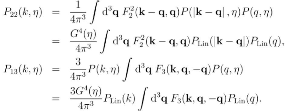
The next order contribution to the power spectrum from PT expansion is the sum of two terms, each one of which mixes up two linear power spectra, PPT(1) =P22+P13 where [27]
P22(k, η) = 1 4π3
Z
d3qF22(k−q,q)P(|k−q|, η)P(q, η)
= G
4(η) 4π3
Z
d3qF22(k−q,q)PLin(|k−q|)PLin(q), (1.54a)
P13(k, η) = 3
4π3P(k, η)
Z
d3qF3(k,q,−q)P(q, η) = 3G
4(η)
4π3 PLin(k)
Z
d3qF3(k,q,−q)PLin(q). (1.54b)
And in this way one can continue up to any order desired.
The linear power spectrum and the first three perturbation terms as computed in the framework of PT just depicted above are shown in the left panel of figure 1.1 as a function of the wave-number. Solid and dashed lines denote positive and negative contributions. This figure shows the main problem of PT: with the exception of the linear power spectrum, each term has both positive and negative contributions and does not appear a tendency for the different perturbative contributions to decrease in amplitude with increasing order. This left us with the impossibility to predict the sign and amplitude of any term before computing it explicitly, and consequently makes the decision of where to truncate the PT expansion problematic. By this fundamental reason one finds the statement on the literature that PT can be used to describe only the mildly non-linear regime but not the full non-linear regime, see [29, 30] and references therein.
1.2 Cosmological perturbation theory 17
Given that the modeling of the two-point statistics of different cosmic fields used in this work requires the proper introduction of the effects of the non-linear evolution of density fluctuations (for the details see §4.1.2 and [8, 7]), in this work we made use of the renormalized perturbation theory (RPT) approach [29,30] as an approach to improve PT results. It is out of the scope of the present work to make a detailed review of RPT, which requires a high level of technical developments and tools of field theory. However, we try to mention the main features and basis of this approach. We closely follow the treatment presented on §2.2 of [6], which can be consulted for detailed discussion.
In an oversimplified way, RPT can be understood as a reorganization of the terms in the PT expansion that remove the problems of this formalism mentioned above. The first idea is that all the terms in the PT expansion for the power spectrum that are proportional to the initial power spectrum, here P(k, t), like P13 (see equation (1.54b)) andP15(see e.g., [27,29]), are grouped together into a common factorG(k, t), the so-called
renormalized propagator, which can be interpreted as encoding the loss of information of the initial conditions due to non-linear evolution. At very large scales, the low-k limit, the renormalized propagator should evolve as the growth factor, G(k, t) ≈ G(t), having no dependence on the initial conditions. Meanwhile, at small scales, the high-k limit, the behavior of the propagator was computed on [29] to have approximatively the form of a Gaussian with zero mean and dispersion given by a characteristic scale determining where linear theory breakdown. Here we call this scale as rNL following [12]8
r2N L = 1 3
Z
dk PLin(k)
k2 . (1.55)
That is, for small scales [30]
G(k, η)≈G(η) exp
−12k2rNL2 (G(η)−1)2
, (1.56)
with G(η) the linear growth factor.
The remaining terms, those that are not proportional toP(k, η), are organized accord-ing to the number n of initial modes coupled and grouped into the mode coupling power spectrum PMC(n)(k, t). As an example, the lower order term is the one that couples two initial power spectra, i.e., PMC(2)(k, t). It is given by P22 of PT (equation (1.54b)) [30]. In this way, the full non-linear power spectrum in RPT formalism should have the following form
P(k, t) = G2(k, t)PLin(k) +
∞
X
n=2
PMC(n)(k, t) (1.57) The linear power spectrum and the first three perturbation terms as computed in the framework of RPT just depicted above are shown in the right panel of figure 1.1
as a function of the wave-number. Solid and dashed lines denote positive and negative contributions. This figure shows how the main problems of PT are alleviated in the context of RPT each term has positive contributions and appears dominant over a restricted range of wave-numbers, which shows a tendency to increase in the values of k with increasing perturbative order. This shows the advantage of RPT over standard PT. In principle, it is simpler to decide where to truncate the series of equation (1.57) if a given precision at wave-number k is required.
8
Note that this quantity have different names on different works, [30] originally call itσv and [8] call
1.3
The Dark Energy Survey
The Dark Energy Survey (DES) is a new generation galaxy survey designed to study the late cosmic acceleration of the Universe through the dynamics of the expansion and the growth of structures at large scales on cosmological context. The DES is a collaboration of over a hundred researchers from the USA, UK, Spain, Germany, Chile, Switzerland and Brazil.
The main innovation in the project is the development of a new optical CCD camera of 5000 megapixels and 2.2 degrees of field of view called DECam, which has been placed at the Blanco 4 meters telescope located at Cerro Tololo Inter-American Observatory (CTIO) in Chile and saw its first light in September 2012. For over five years it will use 30% of the telescope available time to carry out a wide-area survey and reach redshifts 0.2 ≤ z ≤ 1.3−2 with a depth of ∼ 24 in magnitude in SDSS broad bands, g = 24.6,
r= 24.1, i= 24.3 and z = 23.9 over 5000 deg2 in the southern galactic sky.
The DES is expected to detect∼100000 optical galaxy clusters and to measure shapes, redshifts and positions of ∼ 200 millions of galaxies of all types. It will obtain cosmo-logical information about the physical nature of dark energy via four different methods (cosmological observables):
1. Count and spatial distribution of galaxy clusters with 0.2≤z ≤1.3, 2. the evolution of the angular clustering of galaxies,
3. weak lensing tomography up to z ∼1 and
4. distances and luminosities of supernovae in 0.3≤z ≤0.8
While observations and data analyses proceed by different working groups in the col-laboration, simulations are also performed to validate the analysis tools and forecast results with higher confidence. In this work, we will make use of these simulations in order to test pipelines that estimate the angular correlation function of galaxies and how to extract cosmological information from a Bayesian analysis of the data.
1.4
LSS cosmological observables
This section introduces the basic cosmic fields whose correlations will be studied in the remaining of this work. Namely, the angular fluctuation of the density of galaxies in the Universe and the convergence and shear fields that characterize weak lensing phenomena. This will be done from a point of view as general as possible, within a cosmological model based on first order (linear) scalar perturbations around a FLRW model. It will not be assumed from the beginning that the Universe is spatially flat, which will nonetheless be a particular and important case of the treatment here presented.
1.4.1
Three and two-dimensional galaxy clustering
1.4 LSS cosmological observables 19
In order to confront theoretical model predictions for the total mass distribution in the Universe against observational data, a relationship between the fluctuation fields of galaxies and the total matter becomes necessary. The problem appearing resides in the fact that luminous astrophysical objects, such as galaxies and quasars, are not direct (but
biased) tracers of mass in the universe. A difference of the spatial distribution between luminous astrophysical objects and the total matter in the Universe has been indicated from a variety of observations. This difference is commonly referred to in the literature as the biasing effect. It is beyond the scope of this work to present a detailed discussion of galaxy bias modeling. However, some related ideas are presented below.
In common applications a linear biasing model is often assumed in which the fluctua-tion fields of galaxies δg and total matter δm are assumed to be deterministically related by
δg =bgδm, (1.58)
where the bias factor bg fully determines the biasing effect. However, this modeling for the biasing is not based on any reasonable physical motivation. Note that, if the bias factor satisfies bg > 1 everywhere the model should break down because values of the galaxy fluctuation fieldδg below −1 are forbidden by definition, even in voids.
A better motivated and formulated approach to biasing effect is based on the biasing of density peaks in a Gaussian random field (see [31]). In this scheme the galaxy-galaxy and total matter two-point correlation functions, ξgg and ξmm respectively, are related in linear theory by
ξgg=b2gξmm, (1.59)
where the galaxy bias parameter is a constant independent of scale, i.e. ascale independent bias. Note that the relation (1.59) follows from (1.58), but the reverse is not true.
In this work a scale independent galaxy bias of the form (1.58) is used. This relation is assumed phenomenologically for a galaxy population and the bias factor is allowed to vary with the radial distance to galaxies, i.e. with redshift or cosmic time.
The key concept on the theoretical interpretation of angular clustering of galaxies is the field ofprojected galaxy density fluctuation onto the sky orprojected galaxy fluctuation
for short, denoted hereδ2D
g (n). Heren= (θ, ϕ) represents a particular direction (from the observer) on the sky. It is convenient to define it as a properly weighted marginalization of the total galaxy fluctuation on the observer past light-cone,δg(χ(z),n), over its redshift (radial) dependence (see e.g. [7,8, 32]),
δg2D(n) :=
Z ∞
0
dz φg(z)δg(χ(z),n), (1.60) and should be interpreted as the total averaged galaxy fluctuation on a given direction on the sky. The marginalization kernel is the radial selection function of galaxies, φg(z), which describes the selection of galaxies in redshift and depends on the kind of observation considered. It should take into account the sky coverage for the definition of the field, the method used to estimate the redshift of galaxies, spatially varying magnitude limits, etc. The goal here is to derive the relation between the projected galaxy fluctuation δ2D g and the total matter fluctuation today, δ0(χ, θ, ϕ). This theoretical relation should then enable us to relate their statistical properties too. In order to find this relation it is necessary to deal with the proper relation between δg and δ0, which is a non-trivial one.
studied by [33, 34]. In other words, the peculiar velocities of galaxies on top of their background Hubble flow introduce a radial anisotropic distortion in redshift-space (rs), the space of measured positions of galaxies. That is, the redshift distance of a body will be altered from its true distance, by its own peculiar velocity radially oriented from the observer. This deviation alters the apparent clustering of galaxies and, collectively, the effect is said to be the result of redshift space distortions (see Appendix C or classical references, e.g. [33, 34]).
In linear cosmological perturbation theory on a FLRW Universe, the observed redshift-space fluctuation of galaxiesδg(rs) is related to the total matter fluctuation todayδ0 by the
redshift space distortion operator, Rbg, an integro-differential operator, such that, on large scales (see Appendix Cfor a detailed discussion)
δg(rs)(χ,n) = bg(z)G(z)Rbg δ0(χ,n), (1.61) wherebg(z) represents thescale-invariant galaxy bias andG(z) the growing mode of linear matter fluctuations dynamics.
A general treatment of redshift space distortions sourced by Doppler effect in the context of GR is presented on AppendixC. There, the general form for the redshift space distortion operator Rbg is deduced assuming linear perturbation theory and linear scale-independent biasing, and is valid for arbitrary radial separation between the observer and the galaxy (arbitrary galaxy redshift) and also arbitrary spatial curvature. The resulting operator is given by equation (C.36), reproduced here for completeness:
b
Rg =b1 +βg(z)
(
|K|[∂χ+α(χ)]∂χ ∇2+ 3K
−1
K 6= 0,
[∂χ+α(χ)]∂χ ∇2
−1
K = 0,
whereb1 represents the identity operator,βg(z) (equation (C.37)) is the standard
redshift-space distortion factor, determining the strength of the distortions, andαis an observation-dependent function of the comoving distance given by equation (C.29).
Thus, the projected galaxy fluctuation can be written as the projection of the redshift-space distorted fluctuation of matter today,
δ2Dg (θ, ϕ) =
Z ∞
0
dz Wg(z)Rbgδ0(χ, θ, ϕ), (1.62) where the galaxy window function was introduced as
Wg(z) :=φg(z)bg(z)G(z). (1.63)
1.4.2
Weak gravitational lensing
In this section, the first Greek indices α, β, δ . . . run in 2,3 labeling coordinates used to cover the unit sphere S2. Unless mentioned otherwise, the system of usual spherical
coordinates (θ, ϕ) is used, so that the metric is given by [gαβ] =
1 0
0 sin2(θ)
. (1.64)
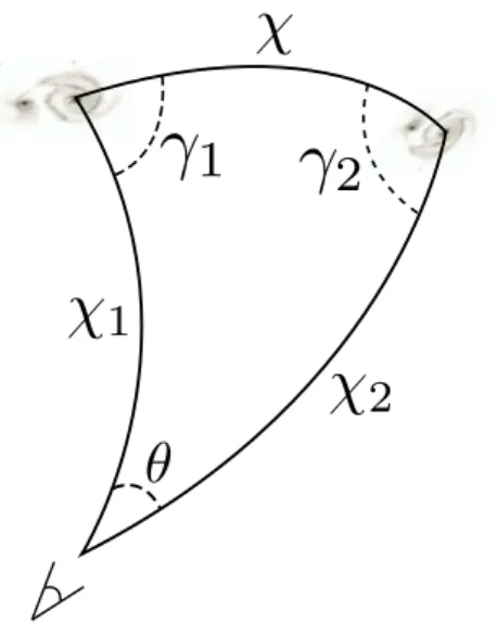
1.4 LSS cosmological observables 21
of the Weyl or lensing gravitational potential, ΨW := (Φ + Ψ)/2, evaluated along unper-turbed radial null geodesics,
(θ−θ0,sinθ0(ϕ−ϕ0)) =αβ =−2
Z rs
0
dr fK(rs−r) fK(rs)fK(r)∇
βΨ
W(η0−r, r, θ0, ϕ0), (1.65) where the sub-indices “s” and “0” denote source (emission of the light ray) and observer (reception of the light ray events) and the function fK is given according to the radial components of the RW metric (equation (1.6)) in coordinatesxµ= (η, r, θ, ϕ) by equation (1.7). The gradient on S2 on (1.65) can be interpreted as a perpendicular gradient to
radial null geodesics in the FLRW background. An explicit computation of the deflection angle (1.65) is presented in Appendix D.
The lensing potential ψ is introduced as
ψ(n0) = 2
Z rs
0
dr fK(rs−r) fK(rs)fK(r)
ΨW (η0−r, r,n0), (1.66) where n0 = (θ0, ϕ0) is a direction on the observer sky, a point on S2, in other words, it is a scalar field onS2 such that its covariant gradient gives the deflection angle of light rays
traveling from the source radial position,rs, to the observer position, r0 = 0 (assumed to be the origin of radial coordinates without loss of generality), i.e.
αβ(n) = −∇βψ(n). (1.67)
Note that the lensing potential depends on the observation timeη0 and the source radial position rs.
The angular coordinates n0 in the deflection angle and the lensing potential expres-sions, (1.65) and (1.66), respectively, represent the undeflected angular position of the source, so that the application
(θ0, ϕ0)7→(θs, ϕs) = (θ0, ϕ0) +α(θ0, ϕ0) = (θ0, ϕ0)− ∇⊥ψ(n) (1.68)
defines what in the literature is called thelens map. In other words, the lens map defines the application that takes the actual angular position of a source in the Universe to the observed deflected position.
The magnification matrix A is defined locally via the covariant derivative of the lens map (1.68), i.e. the Jacobian of the transformation
Aαβ =δαβ− ∇α∇βψ(xδ) =δαβ−2
Z rs
0
dr fK(rs−r) fK(rs)fK(r)∇α
∇βΨW(η0−r, r, xδ)
:=
1−κ 0 0 1−κ
−
γ1 γ2
γ2 −γ1
=
1−κ−γ1 −γ2 −γ2 1−κ+γ1
. (1.69) Note that formally the magnification matrix is defined as a second-rank tensor on S2.
The magnification matrixAdescribes the deformation of a bundle of light rays incom-ing to an observer from a direction n (= xδ) in the sky, i.e. it describes how sources are locally deformed under the lens mapping. This is better understood in equation (1.69), where the separation into trace and trace-free parts is introduced in order to define the scalar fields κ and γ1,2. The former is the S2-divergence of the deflection angle,
κ:= 1 2∇α∇
![Figure 4.3: Impact of different cosmological parameters on the ACF. Each panel shows the the impact of one parameter on the ACF computed for a photometric redshift bin defined by z phot ∈ [0.45, 0.50] with no selection effect on photometric redshift other](https://thumb-eu.123doks.com/thumbv2/123dok_br/18464478.365436/79.892.104.751.109.959/different-cosmological-parameters-parameter-computed-photometric-selection-photometric.webp)
![Figure 4.6: Radial selection functions for the different photo-z bins considered in the SDSS-III DR8 analysis [69]](https://thumb-eu.123doks.com/thumbv2/123dok_br/18464478.365436/88.892.309.549.844.1075/figure-radial-selection-functions-different-photo-considered-analysis.webp)