Pró-Reitoria de Pós-Graduação e Pesquisa
Programa de Pós-Graduação
Stricto Sensu
em Economia
MODELING EXCHANGE RATE DEPENDENCE THROUGH VINE
COPULAS
Brasília - DF
2014
VINÍCIUS MEDEIROS DE LIMA
MODELING EXCHANGE RATE DEPENDENCE THROUGH REGULAR VINE COPULAS
Dissertation submitted in partial satisfaction of the requirements for the degree of Master Science in Economics by the Catholic University of Brasília.
Advisor: Professor Osvaldo Candido da Silva Filho, PhD Board Members: Professor José Ângelo Divino, PhD Aquiles Rocha de Farias, PhD
7,5cm
Ficha elaborada pela Biblioteca Pós-Graduação da UCB
L732m Lima, Vinícius Medeiros de.
Modeling exchange rate dependence through regular vine copulas. / Vinícius Medeiros de Lima – 2014.
37 f.; 30 cm
Dissertation (master's degree) – Universidade Católica de Brasília, 2014. Academic advisor: PhD. Osvaldo Candido da Silva Filho
1. Economy. 2. Exchange rate. 3. Regular vine. 4. Financial analysis. I. Silva Filho, Osvaldo Candido da, academic advisor. II. Title.
Dissertation of the author Vinícius Medeiros de Lima, entitled “Modeling Exchange Rate Dependence through Regular Vine Copulas”, presented as a partial requisite for
obtaining the degree of Master of Science in Economics of the Catholic University of Brasília, in 2014/03/26, defended and approved by the examining board below signed:
________________________________________________ Professor Osvaldo Candido da Silva Filho, PhD
Advisor PPGE – UCB
________________________________________________ Professor José Ângelo Costa do Amor Divino, PhD
Member PPGE – UCB
________________________________________________ Aquiles Rocha de Farias, PhD
Member
Banco Central do Brasil - BCB
ACKNOWLEDGEMENTS
This work is fruit of a knowledge construction which results from the support of those close to me that helped with their knowledge, incentive, perseverance or even patience.
I thank the CNPq – Brazilian National Council of Scientific and Technological Development
by the scholarship, without it I would not have the opportunity to initiate this Master’s
program.
I thank my parents, for whom I also dedicate this work, that educated me to always follow my goals despite the obstacles. Without them, the dream of this title would not even be tangible, their help and support was always the stepping stone for all my small and big realizations. For everything, I thank them.
I thank Professor Osvaldo Candido da Silva Filho, PhD. Not only for the orientation in this
work but for all the attention in the Master’s course and for the always gentle and friendly
company. As well as the opportunity to learn the basics of being a teacher in the monitorship
of the discipline Mathematics I, for the Master’s Program.
I thank Professor José Ângelo Costa do Amor Divino, for the opportunity of getting some teaching experience as a substitute teacher in the discipline of Econometrics II to the graduation of the Catholic University of Brasília, for the gentle participation in this work’s examining board and for all the attention and patience.
I thank the staff of the Budget and Planning Department of the Brazilian National Agency of Land Transportation – GEPLA/ANTT, for the comprehension.
I thank my girlfriend Maria Fernanda Jaloretto, by the pleasure of her companionship, unconditional support, perseverance and patience with the moments of despair and fatigue.
I thank the remarkable sociologist and brother Luiz Gustavo Medeiros de Lima, for believing and making me believe this work was possible.
ABSTRACT
Reference: LIMA, Vinicius Medeiros. Modeling Exchange Rates Dependence through Regular Vine Copulas. 36p. Dissertation of Master Science in Economics – Catholic University of Brasilia, Brasilia, 2014.
The importance of exchange rates to the global economy is proved by the huge volume of negotiation they hold. Being an important macroeconomic variable and, sometimes, tool, as well as an asset, the analysis of FX (Foreign Exchanges) behavior can be a challenge. However, some dependence measures, as the Copula Functions modeled via Regular Vines for a higher number of currencies, can make this task achievable. This work presents a literature review of cointegration, long memory behavior and the self-similarity aspect of Brownian motion. Then introduces the Copula Functions and Vine Copula structures used in recent papers that refers to dependence among time-series. The discussion of R-Vine estimation starts from some basic graph theory concepts to the complex set of copula equations and bivariate conditional densities which are made accessible via the R-Vine. Then, to a broad set of exchange rate series, some economic interpretations are taken from both the structure of the R-Vine and its Copula families and Kendall’s Taus.
RESUMO
CONTENTS
Introduction ... 10
2. Literature Review ... 12
3. Regular Vine copula, estimation procedures and dependence measures ... 17
3.1. R-VINE COPULAS ... 17
3.2. ESTIMATION AND INFERENCE ... 18
3.2.1. Marginal modeling ... 18
3.2.2 R-Vine copula modeling ... 20
4. Results ... 22
4.1. HURST’S EXPONENT ESTIMATION ... 22
4.2. MARGINAL GARCH/FIGARCH MODELING. ... 24
4.3. REGULAR VINE COPULA RESULTS ... 25
5. Final remarks ... 32
References ... 34
If in other sciences we should arrive at certainty without doubt and truth without error, it behooves us to place the foundations of knowledge in mathematics.
10 INTRODUCTION
It is hard to overestimate the importance of exchange rates in a globalized economy. They affect output and employment through real exchange rates; inflation through the cost of imports and commodity prices; international capital flows through the risks and returns of different assets. Given that great participation as a macroeconomic variable and, sometimes, macroeconomic instrument, the trading volume of foreign exchanges is expected to be huge.
The trading volume has exploded reflecting an electronic revolution that has lowered trading costs, attracted new groups of market participants and enabled aggressive new trading strategies. The US dollar alone, in 2010, had a daily average turnover estimated at $ 2.0 trillion, 16 times the combined daily GDP of the world’s 35 largest economies, and roughly
10 times exchange-traded equity turnover (King, Osler and Rime, 2012). The BIS FX Survey 2013 shows that transactions with the US dollar in one of the counterparts respond to 87% of
all foreign exchange trading volume. The dollar’s dominance reflects the market’s practice of
trading minor currencies via a major currency (called the vehicle currency).
This dissertation models the R-Vines for fourteen exchange rate series. Each series are
given by the country’s currency related to the US dollar, were used the Euro (EUR), Great Britain’s Pound (GBP), Japanese Yen (JPY), Indian Rupee (INR), South Korean Won (KRW), Singaporean Dollar (SGD), Swiss Franc (CHF), Swedish Krone (SEK), Norwegian Krone (NOK), Australian Dollar (AUD), Brazilian Real (BRL), Mexican Peso (MXN),
Canadian Dollar (CAD) and the South African Rand (ZAR). Using EMH’s recommendations,
the log-return of these series was used.
Briefly, the main contributions of this work are: use a broader set of FX time-series to further prove that some behaviors are present not only in the main world currencies; and to get some economic interpretation from the R-Vines here modeled.
11
Thus, in an efficient market, models for asset pricing are concerned with the arrival of new information which is taken to be independent and random.
Econometrically, the EMH is consistent with the random walk hypothesis, in which the future behavior of financial series cannot be predicted. A time-series has the random walk characteristic if it has the unit-root property. This property is the starting point of the studies this dissertation shows.
The order of integration of a time series denotes the minimum number of differences required to obtain a covariance-stationary series. A random process with unit-root property, i.e. an I(1) process, is first-order integrated. Given, for instance, two I(1) process, if exists a vector of coefficients forming a linear combination of them that is stationary, then the two I(1) processes are said to be cointegrated and the that vector is called cointegrating vector.
The literature review starts with the cointegration concept. Although, some mistaken implications could be taken when, for instance, an IGARCH model is used. Later, in the literature, the concept of fractional integration was developed and it is closely related to the long memory property – order of integration , with and zero converging variance with divergent sums of these variance terms, respectively.
The long memory property is, also, related to the self-similarity characteristic of the
Brownian motion, and a significant way of detecting long memory is using Hurst’s exponent.
This property will be further explained in the literature review, but it’s main characteristic is
the slow decay of the covariance of the series, in an univariate analysis.
Sometimes, however, it is important to analyze the dependence among two or more processes, in an idea of co-movement. This is where the Copula function is important, it is simply a function of the marginal probability density functions of each process, that returns the joint probability density function. Although it is a very useful way of measuring dependence, it can become too complex to deal with in higher dimensions, in other words, with a great number of processes. To solve this problem, the Copula literature has sought help in the graph theory, with the Pair-Copula Constructions.
The Pair-Copula Constructions (PCC) reveals the relationships among copula
functions, pair to pair, using the graph theory’s concept of Vines. They can be Drawable
12
complex set of equations or matrixes can be showed with a simpler graph, divided in trees, one for each degree of dependence.
The following is a brief summary of the remainder of the paper. Section 2, the literature review, gives the background on exchange rate modeling, from the early studies of cointegration, through the long memory property, Brownian motion and some remarks on pair-copula constructions. Section 3 introduces the methodology used for modeling our mean and volatility equations, the long-memory property estimation and Hurst exponent, and the sequential method for the Pair-Copula Construction (PCC) and R-Vine estimations. With this in hand, section 4 outlines the results found, its econometric and economic implications. Finally, section 5 presents the conclusions of this work. Also there is an appendix with the densities of the Copula functions used in this dissertation.
2. LITERATURE REVIEW
The study of cointegration in exchange rate series started with Baillie and Bollerslev (1989), they used a series with seven spot daily exchange rates, all related to the US Dollar (Canadian Dollar, French Franc, German Mark, Italian Lira, Japanese Yen, Swiss Franc and British Pound). Then, they estimated a VAR (Vector Autoregressive) of p-th order and 7 dimensions, one for each currency.
Their results showed that if considered individually, these series showed unit-root property, but they cointegrate. At this paper, the unit-root property became universally accepted for high frequency asset series.
However, this cointegration was described as fragile in Sephton and Larsen (1991). In such way that different conclusions could be found considering the same sample in different time intervals. So the idea that the usual unit-root tests may lead to a mistaken result begins at this paper. They could result in a unit-root to a well-specified stationary series with structural changes.
13 prediction error. They conclude that: “There´s substantial uncertainty about the existence of
cointegration among spot daily exchange rates with US dollar”.
They also suggest that the cointegration do exist, but it´s not independent in the long
run. This cointegration is associated with long memory models and can be named “fractional cointegration”. A long memory behavior can be graphically illustrated by the Autocorrelation Funcion (ACF) and Partial Autocorrelation Function (PACF) plots. A stationary process has long memory if its ACF has a slow decay and convergence.
Baillie (1996), when defining a Fractionally Integrated Auto-Regressive Conditionally Heteroskedastic process (FIGARCH), shows that the parameter of a poorly specified GARCH model is usually next to the unity, property of an IGARCH behavior as well. So, the unit-root property may not be legitimate and the IGARCH process can lead to mistaken analysis, when compared to long range memory process of conditional variance.
Econometrically, long memory is a halfway house between the usual exponential rates of decay associated with the class of stationary and invertible ARMA models, and the alternative extreme of complete persistence associated with integrated unit root processes (Baillie, 2007)
Long range dependence phenomenon is said to occur when the covariance between and tends to zero but so slowly that their sums diverge. (Prakasa Rao, 2003). Long range dependence is related to the concept of self-similarity for a stochastic process in that the increments of a self-similar process with stationary increments exhibit long range dependence.
A stochastic process is said to be “self-similar” if, for any , there exists such that:
14
A Gaussian process H-ss with stationary increments and with fractal index is called a fractional Brownian motion (fBm). If H = ½, the fractional Brownian motion reduces to a Brownian motion. (Blackledge, 2010)
One of the characteristics of the Brownian motion is the self-similarity. For some financial data and in this work, Hurst exponents for high frequency financial series usually are in the range of 0.5 < H < 1, indicating a persistent time series and the mean-reverting characteristics, indicating self-similarity as well. As seen, there’s a relation between self -similarity and long range memory dependence and this scaling exponent is the first clue of this behavior.
Applying the statistical concepts to finance, can be said that a stochastic process is said to be self-similar with parameter H, if and have the same finite dimensional distribution for all A > 0, with the same long memory parameter across aggregations (Baillie, 2004). In other words, series with intraday, daily, weekly, monthly or annual data may have the same finite dimensional distribution.
The dependence between two different processes can prove some expected behavior or even reveal some unknown characteristics of those time-series. Also, in many fields of knowledge, a univariate analysis can lead to inconclusive or even mistaken conclusions. Hence the crucial importance of a dependence measure between two processes that has been solidified by the Copula function.
As said, Copula functions measure the codependence between probability distributions, it analyses the conjunct behavior of some random variables (RV), the influence of one RV on another. In economic theory, deterministic or econometric models of RV in panel-data or cross-section explain relations between economic variables, like in some empiric models like Phillips curve. The copula may add this dependence study to these variables in time series and show a different treatment to the same issues.
From Sklar’s theorem, x1, ,xnrandom variables with marginal distributions Fi
,with probability density function fi( ) , i1,...,n, and joint distribution F
, there’s acopula function , such that F
x1,,xn
C
F1
x1 ,F2 x2 ,,Fn
xn
and its joint15
x xn
c n
F
x Fn
xn
f x fn
xnf 1,, 12 1 1 ,, 1 1 .
A useful property of copula functions is their invariance towards monotonic transformations of the marginal probability density functions and . In other words, the copula of two marginal distributions is the same for any monotonic transformations. Also, association measures like rank correlation, tail dependence or
Kendall’s Tau may be expressed using copulae. (Morales-Napoles, 2008) Hence it’s
advantage over a linear correlation analysis.
However, for a greater number of processes being tested for dependence, the set of copula equations and bivariate conditional densities may become too complex to work with. In order to simplify the analysis, an aid from graph theory is used.
To illustrate this complexity, we will take the recursive decomposition of the conditional distribution of given as: (Czado, 2012)
For t = 2, … d, Czado (2010) showed that the joint distribution is
Given the simplification necessity, the decomposition in pairs of copulae (or Pair-Copula) may be represented in a sequence of non-oriented nested trees, called vines, which will be defined and discussed later. In finance literature, the copula functions are being used mainly in their bivariate form, called Pair-Copula Construction (PCC). This structure uses tree models, from graph theory. The Regular Vine (R-Vine) is the most flexibly of these structures, and the Canonical Vine (C-Vine) and Drawable Vine (D-Vine) are subclasses of Regular Vines (Bedford and Cooke, 2001; Czado, 2012)
16
17 3. REGULAR VINE COPULA, ESTIMATION PROCEDURES AND DEPENDENCE MEASURES
In this section, some definitions related to Regular Vine copulas are presented along with the methodological procedures used in the empirical study.
3.1. R-VINE COPULAS
Definition 1: Non-Oriented Graph (Gross, Yellen and Zhang, 2005)
A non-oriented graph G = (N,A) consists in a finite and non-empty set N of nodes (also called
points or vertices) and a set E of edges (also named lines or arcs), where each element is a
non-ordered pair of different individuals that are also elements of N.
Definition 2: Tree (Gross, Yellen and Zhang, 2005)
A tree is a non-oriented graph, with no cycles and connected. Considering that T = (N,E) is a
non-oriented graph, the following are equivalent:
1. T is a tree;
2. Any pair of nodes (v, w) of T is connected by only one edge.
3. T is connected. That is, removing an edge disconnects the graph.
Definition 3: Vines (Gross, Yellen and Zhang, 2005)
Vines are non-oriented graphs that specify a joint multivariate distribution. They are sets of
nested trees and have been used to represent higher dimensions probability distributions.
Definition 4: Regular Vine (R-Vine) (Bedford and Cooke, 2002; Czado, 2010)
A regular vine of d variables consists of the connected trees with nodes and
edges , for , that satisfies:
1. has nodes and edge ;
2. For , the tree has nodes .
3. Two edges in a tree are united in the tree if they share a common node in the
tree .
18
Drawable Vine (D-Vine): if each node T – 1 has a maximum of two edges. Commonly
is said that a D-Vine has a straight path structure;
Canonical Vine (C-Vine): if each tree has only one node with d – i edges. This node is called the root of the Vine. Commonly is said that a C-Vine has a star structure.
Definition 5: Regular Vine (R-Vine) Copula (Dißmann, Brechmann, Czado and Kurowicka,
2012)
(F, V, B) is an R-vine copula specification if F ( ,..., )F1 Fn is a vector of continuous invertible distribution functions, V is an n-dimensional R-vine and
e| 1,..., 1; i
B B i i eE is a set of copulae with B being a bivariate copula, a so-called e pair-copula.
3.2. ESTIMATION AND INFERENCE
For GARCH estimation, the statistical software used was R, with the Fgarch package. Taking the usual concept model to financial data, we used a log-return series with both weekly and daily frequencies.
3.2.1. Marginal modeling
The weekly series had a GARCH(1,1) model with some series having some mean equation as well (Brazilian Real, South African Rand and Indian Rupee also had a ARMA(1,1) mean equation).
For daily series, however, the stable GARCH(1,1) estimation was not viable. As seen in literature review, the parameters of this GARCH estimation were usually next to the unity, although these models did not pass in the usual tests of viability. An IGARCH would be the
next model used because of the proximity of GARCH’s parameters to the unity.
19
Also, data generated from a process exhibiting long memory FIGARCH volatility may be easily mistaken for IGARCH behavior. For both the mean and the variance, being confined to only considering the extreme cases of I(0) (stationary process) and I(1) (random walk), or the stable GARCH and IGARCH processes can be very misleading when long memory, but eventual mean-reverting processes are generating the observed data.
It’s important to note that GARCH, IGARCH and FIGARCH models belong to the same family of ARCH(∞) models. The FIGARCH model is essentially a generalization of the
IGARCH model, since the differencing parameter is allowed to be fractional rather than unity. Although the FIGARCH model show relatively more memory than the IGARCH model, in other words, hyperbolic memory rather than geometric memory, both models are characterized by summable sequences of lag coefficients for the squared process, converging to unity, independently of the value of the fractional differencing parameter (Baillie and Morana, 2008)
The MA-FIGARCH model is found to provide an excellent description of daily returns data (Baillie, 2007). This article uses a MA(1)-FIGARCH(1,d,0) to estimate daily series using
Chung’s method (Chung, 1999).
After selecting the appropriate ARMA(P,Q)-GARCH(p,q) model. Ljung-Box tests were used to check independence of the estimated standard residuals (Czado, 2008). As will
be seen afterwards, this work has a similar approach, but we estimated the Hurst’s exponent to
determine the long range memory dependence aspects as well.
While an IGARCH model would impose complete persistence in its impulse response weights, the covariance-stationary GARCH model implies relatively rapid exponential decay. The FIGARCH model, however, imposes the slow hyperbolic decay so that the effect of a volatility shock is very persistent, but eventually mean-reverting. (Baillie, 1996)
20 3.2.2 R-Vine copula modeling
Recently, the works in finance using copulas are using R-Vines because they present the higher flexibility with the greater number of structures possible and its estimation has a more operational and objective criteria since the copula structure is estimated by computer algorithms and no more by step by step estimation. (Morales-Nápoles [2008]; Diβmann, Brechmann, Czado and Kurowicka [2012]).
For selecting a possible R-Vine for a chosen data set is necessary to decide the pairs of variables which copulae will be specified. Proceeding in a sequential manner and defining the first tree for the R-Vine, and so on. The trees are selected in a way that the chosen pair-copula model the greatest dependences, pair to pair.
This method, called sequential method, since each tree is examined separately, doesn´t
guarantee a global optimum, with highest likelihood, lowest information criteria (AIC/BIC).
However, Diβmann et al (2012), Czado (2010), Aas et al (2009) e Kurowicka (2012) believe this approach is reasonable because:
The copula families that are specified in the first tree of the R-Vine generally has the greatest influence at the adjustment of the model.
Is more important to model the structural dependence between random variables that have high dependencies correctly, because most of the copula families can model independence and the copula functions for parameters next to independence are very similar.
To real applications, it is natural to assume that the randomness is given by the dependence of some variables and not all of them. So, if you choose the copulae with high dependence in the top trees, the transformed variables to the trees that follow are generally reasonably independent.
The Kendall’s tau is used as a dependence measure because its measuring power does not depend on the assumed distribution and so, it’s especially useful when different non-gaussian copula families are combined. However, the sequential method, works the same way for any
dependence measure used, not only the Kendall’s tau.
The sequential method (Diebmann et al, 2012) starts by selecting the tree that maximizes
21
tree, choose a copula and estimate the correspondent parameters, transforming each one of the marginal distributions in the adjusted copula. With this we have the first tree, with unconditional residuals in the nodes.
For each of the next trees, we follow the same steps: First we calculate the empirical
Kendall’s Tau for each conditional variable pair that may be part of the tree, in other words,
all extremities that obey the proximity condition. Between these edges, select the tree that maximizes the sum of the empirical Kendall’s Tau absolute values. Lastly, for each edge in
the tree selected, choose the conditional copula and estimate the correspondent parameters. Then, transform the marginal distributions using the adjusted copula.
Despite the steps above showed, it’s necessary to select a copula family for each variable
pair. In this work, the following copula families were taken in consideration (more about these copula families in the appendix):
Gaussian/Normal (symmetric, without tail dependence),
T-student (symmetric, with tail dependence),
Clayton (asymmetric, lower tail dependence only)
Gumbel (asymmetric, upper tail dependence only)
Joe (asymmetric, upper tail dependence only)
Given the options, there’s still the problem in deciding which copula has a better adjust to the model. We do that using the AIC and BIC, that corrects for the log likelihood of a copula to the number of parameters. This way, the use of the t-Student, BB1 and BB7 copulae are penalized, if compared to the other copulae, because it is the only family with two parameters in consideration.
The copula selection starts by computing the Akaike selection criteria (AIC) for each family possible, and then the copula with the lower AIC is selected. The independence copula has to be included in the selection by realizing a preliminary independence test based on
Kendall’s Tau as descript in Genest and Favre 1(2007). If the test indicates independence, no other step is taken and the independence copula is chosen.
1
The test exploits the asymptotic normality of the test statistic:
, Where N is
22
Given the methodology used in this section, the next one presents the results obtained as well as some interpretation and issues of these results. One of the main contributions of this work is an analysis of the R-Vines by an economic point of view, instead of the usual strictly quantitative and econometric one, and it is reserved for this next section.
4. RESULTS
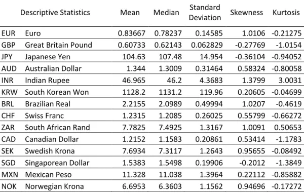
This work used the log-return of 14 spot foreign exchange rates based in the US dollar, with daily and weekly series. The time span starts in 28/12/1999 and goes up to 05/11/2013. The daily series has 3.616 observations of each currency. The weekly one uses the closing rate of Tuesday and has 724 observations.
This section will be presented in the following order: First, the estimation of the
Hurst’s exponent, for mean-reverting and persistence aspects of the sample; then, the GARCH/FIGARCH estimation of each marginal process and finally the Vine Copulas.
Table 1 – Descriptive Statistics
Descriptive Statistics Mean Median Standard
Deviation Skewness Kurtosis
EUR Euro 0.83667 0.78237 0.14585 1.0106 -0.21275
GBP Great Britain Pound 0.60733 0.62143 0.062829 -0.27769 -1.0154
JPY Japanese Yen 104.63 107.48 14.954 -0.36104 -0.94052
AUD Australian Dollar 1.344 1.3009 0.31464 0.58324 -0.80058
INR Indian Rupee 46.965 46.2 4.3683 1.3799 3.0031
KRW South Korean Won 1128.2 1131.2 119.96 0.20605 -0.04699
BRL Brazilian Real 2.2155 2.0989 0.49994 1.0207 -0.4619
CHF Swiss Franc 1.2315 1.2085 0.26025 0.55799 -0.66272
ZAR South African Rand 7.7825 7.4925 1.3167 1.0091 0.50653
CAD Canadian Dollar 1.2152 1.1583 0.20861 0.53414 -1.1783
SEK Swedish Krona 7.6934 7.3117 1.2643 0.95655 -0.08492
SGD Singaporean Dollar 1.5383 1.5498 0.19906 -0.2012 -1.3849
MXN Mexican Peso 11.328 11.038 1.3964 0.22112 -0.85882
NOK Norwegian Krona 6.6953 6.3603 1.1562 0.94696 -0.17272
4.1. HURST’S EXPONENT ESTIMATION
For the Hurst’s exponent estimation, the GRETL software was used, and the results
23
Table 2 –Daily and Weekly Hurst’s Exponent Estimation
Hurst Exponent
Daily Series Weekly Series
EUR 0.54811 (0.0079485) 0.54720 (0.010591) GBP 0.54305 (0.0089423) 0.54904 (0.011719) JPY 0.55624 (0.0076282) 0.59658 (0.011719) AUD 0.53554 (0.0168280) 0.54887 (0.029192) INR 0.61149 (0.0126560) 0.62103 (0.022775) KRW 0.55202 (0.0078384) 0.56235 (0.018146) BRL 0.59361 (0.0091506) 0.65753 (0.012268) CHF 0.54915 (0.0078893) 0.54312 (0.013544) CAD 0.54085 (0.0046198) 0.55405 (0.008571) ZAR 0.59568 (0.0182820) 0.63478 (0.020331) SEK 0.53694 (0.0164270) 0.55262 (0.029639) SGD 0.53349 (0.0074501) 0.54717 (0.011047) MXN 0.52155 (0.0099752) 0.53616 (0.016599) NKK 0.51624 (0.0106730) 0.52747 (0.015329)
It is observed that, based on Hurst exponent regression, all FX series are trend persistent, as H > 0.5 for each of them. However, the results are slightly greater than 0.5. Our series start in the end of the Asian Financial Crisis (1997 – 1999), also an exchange rate crisis took part in Brazil at the period. In 1998, the South African Rand depreciated by 28%, the Reserve Bank raised interest rates by 700 basis points trying to appreciate the South African Rand.
The series ends in November of 2013, and an Indian Rupee crisis was beginning, also the economic recovery of United States from the Subprime crisis of 2008 was in course, thus appreciating the US dollar, and the emergent economies currencies were presenting the most accentuated depreciations.
When H = 0.5, we can say that it is a Random Walk process. Like the movement of a particle suspended on a fluid, the path of a Random Walk process does not suffer from
external perturbations. As can be seen in the table, BRICS’s (BRL, INR and ZAR) exchange
24
4.2. MARGINAL GARCH/FIGARCH MODELING.
Although important for persistence and mean-reverting aspects of the sample, the
Hurst’s exponent does not take into account autocorrelation and heteroskedasticity, hence the
necessity of a GARCH/FIGARCH estimation. In order to model them, the statistical software used was R, with the Fgarch package. Taking the usual concept model to financial data, we used a log-return series with both weekly and daily frequencies. The weekly series had a GARCH(1,1).
To the daily series, however, the stable GARCH(1,1) estimation was not viable. As seen in literature review, the parameters of this GARCH estimation were usually next to the unity, although these models did not pass in the usual tests of viability. An IGARCH would be the next model used because of the proximity of GARCH’s parameters to the unity, but as
seem in the literature review, they could lead into mistaken conclusions. So, this work used a FIGARCH(1,d,1) model for daily data.
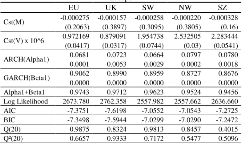
Table 3 – Weekly GARCH(1,1) Estimation
Europe Asia
EU UK SW NW SZ SG JP KO
Cst(M) -0.000275 -0.000157 -0.000258 -0.000220 -0.000328 Cst(M) -0.000219 0.000013 -0.000373 (0.2063) (0.3897) (0.3095) (0.3805) (0.16) (0.0379) (0.9504) (0.0519)
Cst(V) x 10^6 0.972169 0.879091 1.954738 2.532505 2.283444 Cst(V) x 10^6 0.475870 1.632303 2.073541 (0.0417) (0.0317) (0.0744) (0.03) (0.0541) (0.0051) (0.0088) (0.0087)
ARCH(Alpha1) 0.0681 0.0723 0.0664 0.0797 0.0780 ARCH(Alpha1) 0.0868 0.0491 0.2264 0.0001 0.0053 0.0029 0.0002 0.0018 0.0000 0.0023 0.0048
GARCH(Beta1) 0.9062 0.8990 0.8959 0.8727 0.8676 GARCH(Beta1) 0.8592 0.9032 0.7274 0.0000 0.0000 0.0000 0.0000 0.0000 0.0000 0.0000 0.0000 Alpha1+Beta1 0.9743 0.9712 0.9623 0.9524 0.9456 Alpha1+Beta1 0.9460 0.9524 0.9539 Log Likelihood 2673.780 2762.358 2557.982 2557.662 2636.660 Log Likelihood 3204.923 2702.864 2806.554 AIC -7.3751 -7.6198 -7.0552 -7.0543 -7.2725 AIC -8.8423 -7.4554 -7.7419 BIC -7.3498 -7.5944 -7.0299 -7.0290 -7.2472 BIC -8.8170 -7.4301 -7.7165 Q(20) 0.9875 0.8324 0.9813 0.8457 0.4015 Q(20) 0.6306 0.6395 0.0799 Q²(20) 0.6657 0.9333 0.7172 0.5477 0.5096 Q²(20) 0.4307 0.3227 0.9853
BRICS Other Countries
IN BR AF CA AU MX
Cst(M) -0.000247 -0.000266 0.000497 Cst(M) -0.000180 -0.000370 -0.000158 (0.5179) (0.3498) (0.1511) (0.2991) (0.1355) (0.4512)
Cst(V) x 10^6 0.021198 3.528620 0.863237 Cst(V) x 10^6 1.171724 3.661405 1.220636 (0.6197) (0.009) (0.0007) (0.0186) (0.0171) (0.044)
ARCH(Alpha1) 0.1908 0.1837 -0.3020 ARCH(Alpha1) 0.1378 0.1369 0.1402 0.1136 0.0000 0.0712 0.0000 0.0007 0.0169
25
Table 4 – Daily FIGARCH(1,d,1) Estimation
Europe Asia
EU UK SW NW SZ SG JP KO
Cst(M) -0,000147 -0,000115 -0,000183 -0,000138 -0,000192 Cst(M) -0,000093 -0,000039 -0,000147 (0.1484) (0,1886) (0,1214) (0,2594) (0,0915) (0.0545) (0.7046) (0.0347)
Cst(V) x 10^6 132,969342 33,929526 53,421347 49,563306 -673,959920 Cst(V) x 10^6 11,165424 44,870344 22,279907 (0.0892) (0,0006) (0.0000) (0.0000) (0.0001) (0.0008) (0.0000) (0.0361)
d-Figarch 0,918818 0,447267 0,372311 0,324588 1,018618 d-Figarch 0,449389 0,289549 0,493550
ARCH(Alpha1) 0,012638 0,299643 0,272980 0,312152 -0,046092 ARCH(Alpha1) 0,224342 0,438127 0,3130 (0.7438) (0.0000) (0.0000) (0.0000) (0,0294) (0.0000) (0.0058) (0.0000)
GARCH(Beta1) 0,953507 0,716402 0,642468 0,624759 0,965172 GARCH(Beta1) 0,659452 0,662668 0,6597 (0.0001) (0.0000) (0.0000) (0.0000) (0.0000) (0.0000) (0.0000) (0.0000) Alpha1+Beta1 0,966145 1,016045 0,915448 0,936911 0,919080 Alpha1+Beta1 0,883794 1,100795 0,972684 Log Likelihood 13336,068 13733,165 12699,583 12703,962 13010,167 Log Likelihood 15866,070 13184,388 14193,286 AIC -7,3749 -7,5946 -7,0227 -7,0252 -7,1946 AIC -8,7746 -7,290948 -7,8491 BIC -7,3646 -7,5843 -7,0125 -7,0149 -7,1843 BIC -8,7643 -7,280669 -7,8388 Q(20) 0,9133 0,5073 0,8731 0,9936 0,0983 Q(20) 0,0659 0,550020 0,2327 Q²(20) 0,8856 0,7124 0,6589 0,9453 0,6185 Q²(20) 0,9016 0,119727 0,9926
BRICS Other Countries
IN BR AF CA AU MX
Cst(M) -0.000042 -0,000284 0,000770 Cst(M) -0,000058 -0,000193 -0,000089 (0.0881) (0.0146) (0.6183) (0.4929) (0.0871) (0.2666)
Cst(V) x 10^6 2.646509 0,945595 0,666493 Cst(V) x 10^6 14,267074 0,597261 34,839461 (0.1994) (0.0068) (0.0043) (0.0714) (0.0022) (0.0008)
d-Figarch 0.375968 0,543374 0,422361 d-Figarch 0,678253 - 0,356102
ARCH(Alpha1) 0.216525 0.059361 0.282630 ARCH(Alpha1) 0,208759 0,056330 -0,018485 (0.0685) (0.5526) (0.0000) (0.0321) (0.0000) (0.9282)
GARCH(Beta1) 0.406255 0,449030 0,628933 GARCH(Beta1) 0,861297 0,934736 0,249490 (0.0014) (0.0007) (0.0000) (0.0000) (0.0000) (0.2831) Alpha1+Beta1 0.623350 0,508391 0,911563 Alpha1+Beta1 1,070056 0,991066 0,231005 Log Likelihood 16343.887 12437,028 11638,132 Log Likelihood 13902,217 12658,552 13741,754 AIC -9.039495 -6,8775 -6,4355 AIC -7,6881 -7,0011 -7,5993 BIC -9.030930 -6,8672 -6,4252 BIC -7,6778 -6,9943 -7,5890 Q(20) 0.0684 0,5057 0,2760 Q(20) 0,6733 0,5798 0,7773 Q²(20) 0.9979 0,7238 0,6881 Q²(20) 0,3446 0,0702 0,4680
As the GARCH(1,1) and FIGARCH(1,d,1) models were estimated, their standardized residuals were stored and then we used the probability integral transformation that returns uniform distributed marginal standardized residuals. The sequential method for copula selection and structure used these normalized standardized residuals.
4.3. REGULAR VINE COPULA RESULTS
The algorithm presented in Diβmann et al (2012) and showed in the methodology
section was applied via the VineCopula package of the R Software.
26
beyond the third tree the independence copula (identified with a I, 0) becomes the majority of the edges of those trees.
Despite the growing relevance of Vine Copula estimation in recent financial and economic literature, the analysis is often made by a strictly statistical point of view. However, the structure of an R-Vine, as well as the Copula families selected by the algorithm, can reveal some important issues. One of the contributions of this work is the attempt get some interpretations from these R-Vine characteristics.
In the following R-Vines, in each tree we have the currencies in the nodes and the copula families in the edges, which are represented by a letter (N – Gaussian; t – t-student; C
– Clayton; G – Gumbel; J – Joe; see the appendix i for more information) followed by the
Kendall’s Tau of the respective copula, separated by a comma.
First of all, both the daily and weekly R-Vines follow the same structure of nodes,
despite some Kendall’s Tau differences. This is important for the self-similarity characteristic, this result indicates that the series may have the same finite distribution for different time frequencies. One of the surprises of the Vine Copula estimation was the central position assumed by the Singaporean dollar (SGD), as seen in the first tree of each R-Vine.
Graph 1 – R-Vine – Daily Series – Tree 1
27 Singapore’s well known non-internationalization policy illustrates the fact that currency internationalization is not a necessary condition for the development of a financial center (Park and Shin, 2009). Singapore has the third greatest market activity in the world, 5.7% of all FX trading in 2013 occurred via intermediation of Singaporean dealers. Losing only to the United Kingdom (41%) and to the United States (19%), and it has greater activity than Japan (5.6%) and Hong Kong (4.1%).
However, the Singapore Dollar is only the 15th in volume of negotiations (BIS FX Survey, April 2013), it has a higher volume only than the South Korean Won (17th), the South African Rand (18th), the Brazilian Real (19th) and the Indian Rupee (20th).
The isolated Japanese Yen occupies the third greater volume of exchanges
negotiations, losing only to the Euro and US dollar, the negative Kendall’s Tau of the Yen is
due to the depreciation in the Japanese Asset Price Bubble (1986 – 1991) that continued during the period of zero interest rate followed by the Bank of Japan. After the global crisis of 2008, this trend reversed, hence the negative indicator and isolated position in the Vine.
So, despite having one of the most prominent foreign exchange markets in the world, the central position of the Singapore Dollar in the first tree of the R-Vine is a simply statistical fact. The next two trees, giving the conditional copulas, show this effect. Note, for instance,
the Kendall’s Tau between SGD and EUR and the one between SGD and AUD. Then, note
that the Kendall’s Tau, in tree 2 below, between AUD,SGD and EUR,SGD is greater than both of the first tree’s Kendall’s Tau.
This second tree is the first order conditional tree. In order to read this graph, it has to be observed that each edge connects two nodes with one common currency between them. So,
the edge gives the copula family and Kendall’s tau between the different currencies in the
nodes given the common currency in them.
28
currency between the nodes is the Singaporean Dollar (SGD). So, the copula function of both the Australian Dollar (AUD) and the Euro (EUR), conditional to the Singaporean Dollar is a
Gaussian copula, and the Kendall’s Tau is 0.36.
Graph 2 – R-Vine – Daily Series – Tree 2
One of the Copulae that is worth noticing is the one between EUR,SEK and SEK,NKK. A t-student copula with a τ = 0.95. So, the great codependence between the Euro and the Norwegian Krona (NKK) conditional to the Swedish Krona (SEK) demonstrates the
integration amongst these countries. Norway is Sweden’s main export partner and third
greater import partner (CIA World Fact Book), also, both economies are mainly correlated to the Eurozone countries. And given that neither the Swedish nor the Norwegian Krona are
internationalized currencies, the big Kendall’s Tau is fully explained by the close economic
relationship among these countries.
29
Real, conditional to the Australian Dollar. Despite some opinions in favor of Australia joining
the BRICS, there is a hidden BRICS’s Country that may be influencing the behavior: China.
China is Australia’s biggest trading partner (Australian Department of Foreign Affairs
and Trade) and these Sino-Australian economic relations helped Australia to escape the worst effects of the global economic meltdown since 2008. China has helped the BRICS to escape these effects as well. However the Chinese Renminbi or Yuan (CNY) could not be modeled
given China’s Currency Intervention Policy.
The relation between a BRICS’s Country and Australia is also shown in the third tree of
the daily series below. The t-student copula between AUD,KRW|SGD and INR,SGD|KRW
has a Kendall’s Tau of 0.45. This shows the codependence between the Australian Dollar and the Indian Rupee (INR) conditional both to the Singaporean Dollar and the South Korean Won (KRW).
Graph 3 – R-Vine – Daily Series – Tree 3
30
Graph 4 – R-Vine – Weekly Series – Tree 1
As said, both the daily and the weekly R-Vines follow the same structure. The difference
between them is some Copula families and Kendall’s Tau. This contributes to the
31
Graph 5 – R-Vine – Weekly Series – Tree 2
32 5. FINAL REMARKS
This dissertation presents a wider discussion of Pair-Copula Constructions by presenting a broader set of exchange rate series than usual in the literature. It presents 86.5% of all FX trading volume and a total of 15 currencies, including the US dollar. This wider R-Vine can show some particularities of the FX market like: the resemblance of Nordic currencies and the central position of Singaporean Dollar, which indicates some geographic changes in the exchange markets.
In most studies using Pair-Copula Constructions, Vine-Copulas or even single dimension Copulas, the focus is given to the statistical or econometrical analysis. Although these statistical structures have a great use in various fields of knowledge, the economic analysis does not constitute the main goal of those studies.
Our goal here, however, was not to give concrete and absolute explanations about the statistical distribution of the copula functions and the structure of the R-Vine. This research tried, with some level of success, to get some clues from a Vine-Copula structure that, at first
view, wasn’t expected. And from this surprise, to further analyze these economic relations.
This is the differential of the present work. The traditional scientific method constitute in an experiment or tool that is used to prove some previous theory. In this dissertation, however, a relatively recent tool like the Vine-Copula was used to diagnose some FX dependence. And with the R-Vine’s hints, some characteristics unknown by the authors could be researched and found.
Among these great flux of data and information analysis, the debate is still about market efficiency. Maybe the great difference between motion in economic data and data from natural sciences is the influence of previsions on the same data we use to make these same forecasts.
33
34 REFERENCES
Aas, K., Czado, C., Frigessi, A., Bakken, H. (2009) Pair-copula constructions of multiple dependence. Insurance, Mathematics and Economics, 44, 182-198.
Akaike, H. (1974) A new look at statistical model identification. IEEE Transaction on Automatic Control, 19, 716-23.
Baillie, R. T., Bollerslev, T. (1989), The message in daily exchange rates: a conditional variance tale. Journal of Business and Economic Statistics, 7, 297-306
Baillie, R. T., Bollerslev, T., Mikkelsen, H. O. (1996) Fractionally integrated generalized autoregressive conditional heteroskedasticity, Journal of Econometrics, 74, 3-30.
Baillie, R. T. (1996) Long memory processes and fractional integration in econometrics,
Journal of Econometrics, 73, 5-59.
Baillie, R. T., Cecen, A. A., Erkal, C., Han, Y. (2004) Measuring non-linearity, long memory and self-similarity in high-frequency European exchange rates, Journal of International Financial Markets, Institutions & Money, 14, 401-418
Baillie, R. T., Young-Wook, H., Myers, R. J., Song, J. (2007) Long memory models for daily and high frequency commodity futures returns, The Journal of Futures Markets, 27, 643-668.
Baillie, R. T., Morana, C. (2008) Modeling Long Memory and Structural Breaks in Conditional Variances: An Adaptive FIGARCH Approach.
Bedford, T. and Cooke, R.M. (2002). Vines – a new graphical model for dependent random variables. Annals of Statistics, 30(4), 10311068.
35
Blackledge, J. M., (2010) The Fractal Market Hypothesis: Applications to Financial Forecasting, Centre for Advanced Studies, Warsaw University of Technology, vol:
978-83-61993-01-83, pages: 1-105, 2010.
Chung, Ching-Fan (1999) Estimating the Fractionally Integrated GARCH Model, working paper, National Taiwan University.
Czado, C., Min, A., Baumann, T., Dakovic, R. (2008) Pair-copula constructions for modeling exchange rate dependence.
Czado, C. (2010) Pair-copula constructions of multivariate copulas. In Jaworski PEA (ed.),
Copula theory and its applications, lecture notes in statistics, vol. 198. Berlin Heidelberg:
Springer-Verlag, 93-109.
Czado, C., Schepsmeier, U., Min, A. (2012) Maximum likelihood estimation of mixed C-Vines with application to exchange rates. Statistical Modelling, 12, 229 - 255
Diβmann, J., Brechmann, E. C., Czado, C., Kurowicka, D. (2012) Selecting and estimating regular vine copulae and application to financial returns, Computational Statistics & Data Analysis, 59, 52-69, 2013
Einstein, A., (1926, reprinted 1956) Investigations on the Theory of Brownian Movement, ed. R. Fürth, translated by A.D. Cowper; Einstein, Collected Papers, vol. 2, 1-18
Embrechts, P., Maejima, M. (2000) An introduction to the theory of selfsimilar stochastic processes. International Journal of Modern Physics, B 14, 1399-1420
Granger, C. W. J., Ding, Z. (1996) Varieties of long memory models, Journal of Econometrics, 73, 61-77
36
Liu, M. (2000) Modeling long memory in stock market volatility, Journal of Econometrics,
99, 139-171.
Ljung, G., Box, G. (1978) On a measure of lack of fit in time series models. Biometrika, 65,
297-303.
Morales-Nápoles, O., (2010), Bayesian belief nets and vines in aviation safety and other applications. PhD Thesis, Technische Universiteit Delft.
Nikoloulopoulos, A., Joe, H., Li, H. (2011) Vine copulas with asymmetric dependence and applications to financial return data. Computational Statistics and Data Analysis, 56,
3659-3673.
Prakasa Rao, B.L.S. (2003) Self-similar processes, fractional Brownian motion and statistical inference, A Festschrift for Herman Rubin, Institute of Mathematical Statistics, Lecture Notes
– Monograph Series, 45, 98-125
Sephton, P. S., Larsen, H. K., (1991) Tests of exchange market efficiency: fragile evidence from cointegration tests, Journal of International Money and Finance, 10, 561-570.
i
APPENDIX: COPULA FUNCTIONS
N – Gaussian copula
The Gaussian copula is a distribution over the unit cube . It is constructed from a multivariate normal distribution over by using the probabilty integral transform.
For a given correlation matrix , the Gaussian copula with parameter matrix can be written as
where is the inverse cumulative distribution function of a standard normal and is the joint cumulative distribution function of a multivariate normal distribution with mean vector zero and covariance matrix equal to the correlation matrix .
The density can be written as:
T – t-Student Copula
Like the Gaussian Copula, it can be defined from the multivariate normal distribution over , the t-Student distribution generates the t-Copula, which is given by:
Where:
is the correlation matrix;
is a parameter known as degrees of freedom of the t-Student distribution; and
is the cumulative distribution of a univariate padronized t-Student distribution.
Archimedean Copulae
ii
C – Clayton Copula
Bivariate Copula:
Generator:
Parameter:
G – Gumbel Copula
Bivariate Copula: Generator:
Parameter:
J – Joe Copula
Bivariate Copula: Generator: