www.adv-radio-sci.net/11/159/2013/ doi:10.5194/ars-11-159-2013
© Author(s) 2013. CC Attribution 3.0 License.
Radio Science
A first approach to the distortion analysis of nonlinear analog
circuits utilizing X-parameters
H. Weber, C. Widemann, and W. Mathis
Institute four Theoretical Electrical Engineering, Leibniz Universit¨at Hannover, Hanover, Germany
Correspondence to:C. Widemann ([email protected])
Abstract. In this contribution a first approach to the distortion analysis of nonlinear 2-port-networks with X-parameters1 is presented. The X-parameters introduced by Verspecht and Root (2006) offer the possibility to describe nonlinear microwave 2-port-networks under large signal con-ditions. On the basis of X-parameter measurements with a nonlinear network analyzer (NVNA) behavioral models can be extracted for the networks. These models can be used to consider the nonlinear behavior during the design process of microwave circuits. The idea of the present work is to ex-tract the behavioral models in order to describe the influence of interfering signals on the output behavior of the nonlinear circuits. Hereby, a simulator is used instead of a NVNA to ex-tract the X-parameters. Assuming that the interfering signals are relatively small compared to the nominal input signal, the output signal can be described as a superposition of the effects of each input signal. In order to determine the func-tional correlation between the scattering variables, a polyno-mial dependency is assumed. The required datasets for the approximation of the describing functions are simulated by a directional coupler model in Cadence Design Framework. The polynomial coefficients are obtained by a least-square method. The resulting describing functions can be used to predict the system’s behavior under certain conditions as well as the effects of the interfering signal on the output signal.
1 Introduction
A high-frequency circuit can be designed by describing the N-port using scattering parameters (S-parameters) that allow to describe the N-port without current and voltage. Instead alternative variables are used. These variables are called the scattering variables and they are linear combination of the
1X-parameter is a registered trademark of Agilent Technologies,
Inc.
voltage and current of the analyzed N-port. The scattering variables are proportional to the electrical power and are measurable for high-frequencies. However, the S-parameters are restricted to linear and time-invariant N-ports. Thus, they cannot describe nonlinear circuits under large signal excitation. In the last two decades, the description with S-parameters was extended by Verspecht (1995). The linear S-parameters are advanced to the so called X-parameters introduced by Agilent Technologies (Verspecht and Root, 2006). The basic principle is called thepolyharmonic distor-tion(PHD) which allows to describe a nonlinear circuit un-der large signal excitation. Moreover, it is possible to extract the X-parameters using a nonlinear vector analyzer (NVNA) (Roblin, 2011). By this means, a behavioral model for the device under test (DUT) can be developed. This model can be used for the design (Pel´aez P´erez, 2012) or can be added as additional information in the data sheet of an IC producer (Horn et al., 2008). The PHD assumes that only one large signal is applied to the N-port which defines the large signal operating point (LSOP). Other signals are superimposed at an integer multiple of the large signal frequency and are as-sumed as small signals. In this paper, a method is presented for the extraction of X-parameters using a simulator like Ca-dence. Therefore, the extension of scattering variables for nonlinear circuits is reviewed at first.
2 Scattering variables
Before describing a nonlinear N-port with X-parameters, the scattering variables are introduced. Therefore, the behavior of scattering variables for a nonlinear circuit have to be ex-amined. For this purpose, the 1-port in Fig. 1 is given.
The nonlinear impedance in the 1-port is described by
1-port
U
qZ
0i
i
M
u
Fig. 1.Nonlinear resistor regarded as 1-port.
Table 1.Labeling of the scattering variables for a nonlinear 1-port.
Scattering Variable
b11 Asin(ωt )
1−α1Z0−34A2εα3 2√Z0
b13 A3sin(3ωt )Z0εα3
4·2√Z0
a11 2√UqZ
0
Furthermore the mesh
u=Uq−Z0·i (2)
can be set up. Assuming the port voltage to be
u=Asin(ωt ), (3)
one can insert these equations into the definitions of the scat-tering variables
a:=u+Z0·i
2√(Z0) =
Uq 2√Z0
(4) and with Eq. (1)
b: =u−Z0·i
2√(Z0) =
(1−Z0α1)u−Z0εα3u3
2√Z0 =Asin(ωt ) 1−α1Z0−
3 4A
2εα 3
2√Z0
!
(5)
+A3sin(3ωt ) Z0εα3
4·2√Z0
.
In Eq. (4), one can see that the scattering variablea is in-dependent from the connected nonlinear 1-port. In contrast, the scattering variablebdepends on the connected nonlinear 1-port. Due to the nonlinearity, harmonics can be recognized in Eq. (5). In order to describe this nonlinear effect with the scattering variables, an extended notation is introduced in Ta-ble 1. In addition to the first index, a second one is established to describe the generated harmonics separately according to the fundamental.
In Fig. 2, the scattering variables are represented in the frequency domain in order to illustrate the harmonic frequen-cies.
a
b 1-port
Nonlinear
dB
1 3
dB
1
Fig. 2.Scattering variables represented in the frequency domain for a nonlinear 1-port.
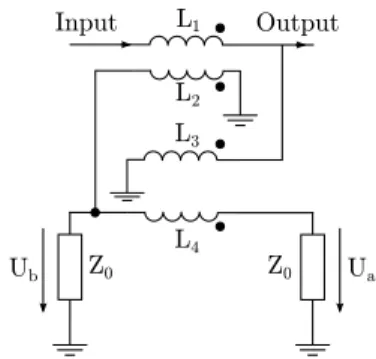
Input 1
L2
L3
L4
Ub Z0 Z0 Ua
L Output
Fig. 3.Directional coupler model to obtain the scattering variables
aandb.
Using the established notation for the scattering variables, it is now possible to describe all frequencies. However, it is still complicated to simulate these scattering variables be-cause they are a linear combination of voltage and current and cannot be measured or simulated in the circuit directly. Therefore, a directional coupler is used in a real environment to determine all scattering variables. In the next section a di-rectional coupler model is illustrated to provide all advan-tages of a real directional coupler in a simulator.
2.1 Directional coupler model
In the measurement technology, a directional coupler is used to obtain the scattering variablesaandb. For simulation pur-pose, there are model approaches to the directional coupler behavior. One possibility of such a model is presented in Fig. 3 (Sierra, 2010).
This model consists of two coupled inductor pairs to trans-fer the current and the voltage which are used to determine the scattering variablesaandb. The dimension of the induc-tor pairs can be determined by the coupling facinduc-tor
C=20 log10
N
2
N1
. (6)
N2andN1represent the number of windings of the coupled
inductorsL1andL2, respectively. By the relation
N2
N1=
s
L2
L1
the inductorsL1andL2can be dimensioned. Furthermore,
L3=L2andL4=L1are assumed. The scattering variables
are represented in this model by the voltagesUaandUb. In order to determine the scattering variables, the voltages have to be multiplied with √1
Z0. In the following, this model will
be used to extract the scattering variables in order to describe a nonlinear N-port with X-parameters.
3 Extension to X-parameter
Certain properties of a linear N-port can be characterized by the parameters. Considering the scattering variables the S-parameters describe the connection between these by
b1
b2
.. . bN
=
S11 S12 · · · S1j
S21 S22 · · · S2j
..
. ... . .. ... SN1SN2· · ·SN N
·
a1
a2
.. . aN
(8)
Furthermore, the behavior of the nonlinear system depends on the excitation. Considering only one generated frequency, the relation between the scattering variableaij andbnmcan be described by
bnm=Fnm(a11, a12, ...a21, a22, ...) . (9)
The nonlinear scattering functionFnm(·)is hard to iden-tify (Sun et al., 2010). However, under certain circumstances, simplifications can be applied. One assumption is that only one of the input signals represented by the scattering vari-ablesaj k is a large signal which is typically defined asa11.
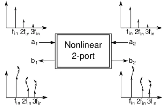
The rest of the signals occur at integer multiples of the large signal frequency with a small amplitude. Considering these assumptions, the system is linearized (Verspecht et al., 2005). Therefore, the superposition principle is valid for the small signals which are superimposed to the LSOP. The principle of the linearization is illustrated in Fig. 4. This allows to re-duce the Eq. (9) to
bnm=
X
j k
Snj,mk(|a11|)P+m−kaj k
+X
j k
Tnj,mk(|a11|)P+m+kaj k∗ (10)
withP =ej ϕa11 for the phase normalization (Verspecht and
Root, 2006). The functions Snj,mk(|a11|) andTnj,mk(|a11|)
are called X-parameters.
For linear systems, the parameters Snj,mk(|a11|) are
re-duced to the linear scattering parameters in Eq. (8). Due to the two tone excitation, intermodulation occurs in nonlin-ear systems. This behavior is represented by the parameters
Tnj,mk(|a11|)that is hence only necessary for nonlinear
sys-tems. Exploiting Eq. (10) and considering the restriction for
aj k6=a11 to be small signals, it is possible to calculate the
behavior of the N-port for multiple input signals.
fin2fin3fin
fin2fin3fin
a2
b2
fin2fin3fin
fin2fin3fin
a1
b1
Nonlinear 2-port
Fig. 4.Superposition for a nonlinear system (Verspecht and Root, 2006).
3.1 Determine X-parameters with a simulator
The X-parameters are extracted in the electrical measure-ment for a nonlinear N-port using a NVNA. In this section, a method to extract the X-parameters by using a simulator like Cadence Spectre is going to be presented. For this purpose, the network is realized in the simulator. The required scatter-ing variables are extracted by the directional coupler model introduced in Sect. 2.1. The structure for the extraction of X-parameters is exemplarily illustrated for a 2-port network in Fig. 5.
At first, the N-port is excited only by the large sig-nal a11. Due to the phase normalization, the X-parameters
Tn1,m1(|a11|)andSn1,m1(|a11|)in Eq. (10) can be
summa-rized toSn1,m1(|a11|). Therefore, Eq. (10) is reduced to
bnm=Sn1,m1(|a11|)Pm|a11|. (11)
The X-parametersSn1,m1(|a11|)can be determined by using
the scattering variablesbnmanda11. Hence, pairs of values of
the scattering variablebnmdepending ona11are necessary.
For a certain range of|a11|, the amplitude and phase of the
scattering variablebnm are determined. The pairs of values are interpolated by the least-square-fit (Herrmann, 2007).
After determining the X-parameters of the large signal, the X-parameters for multiply inputs (Snj,mk(|a11|), k >1) are
determined. Therefore, further signals are used in addition to the large signal. A harmonic balance simulation allows to separate the intermodulation products which are represented by the X-parameters of the small signal. Exemplarily, one can assume that the excitation occurs at the frequenciesfa11=
200 MHz andfa12=400 MHz. If all harmonics of the small
signal at the frequency 400 MHz are neglected it results in three intermodulation products
1·fa11 +0·fa12 = 200 MHz, (12)
(−1)·fa11 +1·fa12 = 200 MHz, (13)
3·fa11 −1·fa12 = 200 MHz (14)
for the scattering variable bn1 at the frequency 200 MHz.
C1 Z0
Uin
Ub1 Z0 Ua1 Z0 R1 R2
Udd
C2
Ua2 Z0 Ub2 Z0 Z0 R3
coupler coupler
NL 2-port
Fig. 5.Structure for the extraction of X-parameters for a 2-port.
0 0,2 0,4 0,6 0,8 1 1,2 1,4 1,6 1,8 2
-160 -140 -120 -100 -80 -60 -40 -20
[dB]
x 109
b2
Frequency [Hz]
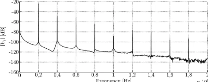
Fig. 6.Frequency domain of the scattering variableb2.
X-parameter. Thus, it is possible to determine each of them separately. The intermodulation product in Eq. (13) is repre-sented bySn1,12(|a11|). In Eq. (14), one can see that the
fre-quency of the small signal frefre-quency offa12is multiplied by
(−1). Since this factor implies the complex conjugate signal
a12∗, the intermodulation product Eq. (14) is represented by
Tn1,12(|a11|). As functional approach for the X-parameters a
polynomial approach is used for the interpolation.
3.2 Description of nonlinear 2-port with X-parameters
In the following, the nonlinear 2-port in Fig. 5 is described by using X-parameters. This example is limited to the de-scription of the scattering variableb21in order to reduce the
effort.
At first, the nonlinear 2-port is excited bya11 at the
fre-quencyfa11=200 MHz. Two directional couplers are used
to extract all scattered variables. Exemplarily, the spectrum of scattering variables|a1|and|b2|are illustrated in Figs. 6
and 7. In the latter, one can see that also harmonics occur in addition to the excitation at 200 MHz. However, as in Eq. (4) calculated, the scattering variablea1depends only on the
ex-citation. Nevertheless, harmonics are still generated due to the imperfection of the directional coupler. In the follow-ing, these harmonics are neglected because the amplitudes are very small. In Fig. 6, harmonic frequencies can be ob-served in the spectrum of the scattering variableb2 which
depends on the nonlinear 2-port as stated in Sect. 2.
In the following, the extraction of the X-parameters of the scattering variableb21will be executed. Therefore, the
non-linear 2-port is only excited bya11at first. Pairs of values of
0 0,2 0,4 0,6 0,8 1 1,2 1,4 1,6 1,8 2
-200 -180 -160 -140 -120 -100 -80 -60 -40 -20
x 109
[dB
]
a1
Frequency [Hz]
Fig. 7.Frequency domain of the scattering variablea1.
0 0,01 0,02 0,03 0,04 0,05 0,06 0,07 0,08 0
0,02 0,04 0,06 0,08 0,1 0,12
b
MATLAB Cadence
21
√
W
[ ]
[ ]
a11√W
Fig. 8.Scattering variableb21simulated and calculated.
a11andb21are simulated and discrete values of the
connect-ing X-parameter is calculated by
S21,11(|a11|)=
b21
a11
. (15)
These values are fitted by a polynomial approach which leads to an approximation of the X-parameter S21,11(|a11|). The
exemplary result is shown in Fig. 8 with the discrete simula-tion values. After determining the X-parameterS21,11(|a11|),
the small signala12is superimposed at the frequency of 400
MHz. In this case, for the scattering variableb21one can say
b21=S21,11(|a11|)a11+S21,12(|a11|)P−1a12
+T21,12(|a11|)P3a12∗ . (16)
The X-parameters S21,12(|a11|)andT21,12(|a11|)are
deter-mined by a harmonic balance simulation. At first, the con-tribution of the intermodulation product in Eq. (13) to the scattering variableb21is calculated. As for the X-parameter
S21,11(|a11|)the pairs of values are fitted by a polynomial
approach which represents the X-parameterS21,12(|a11|)as
well as S21,11(|a11|). The third intermodulation product in
Eq. (14) is represented byT21,12(|a11|). AsS21,12(|a11|)the
X-parameterT21,12(|a11|)is determined by a harmonic
bal-ance and polynomial approach.
In Fig. 9, the simulated (dots) and calculated (plane) scat-tering variableb21 is illustrated depending ona11 anda12.
For small amplitudes ofa12the calculated approximation
co-incides with the simulation whereas for higher amplitudes ofa12one can see a deviation. This behavior is more
0 0,01 0,02 0,03 0,04 0,05 0,06 0,07 0,08
0,025 0,02
0,015 0,01 0,005 0
[ ]
a11 √W a12[ ]√W
0 0,02 0,04 0,06 0,08 0,1 0,12
√
W
b21
[
]
Fig. 9.Scattering variableb21depending ona11anda12.
0 1 2 3 4 5 6 7 8 9 10
x 10-3
0,033 0,034 0,035 0,036 0,037
[ ]
a12 √W
b21
√
W
[
]
MATLAB Cadence
Fig. 10.Scattering variableb21 depending ona12 for fix|a11| =
0.011√W.
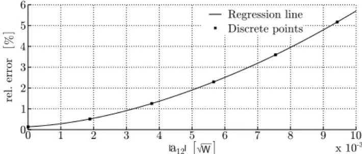
approximation is only valid for small amplitudes of the su-perimposed signals as assumed for the linearization of Eq. (9). In order to demonstrate the difference between simula-tion and approximasimula-tion the relative error is calculated by
rel. error=|bsim−bcal| |bsim| ·
100[%]. (17)
In Fig. 11, the relative error at discrete simulation points is illustrated for the results shown in Fig. 10. A regression line is added to illustrate the tendency. In Fig. 11, it can be seen that the smaller the amplitude ofa12, the better the
approx-imation. However, the relative error raises drastically with increasing amplitude ofa12due to the breach of the
assump-tion of smallaj k6=a11.
4 Conclusion and outlook
In this paper, the description of nonlinear systems with X-parameters using a circuit simulator like CADENCE Design Framework is presented. Therefore, a short introduction of the application of scattering variables on a nonlinear system was given. For the extraction of the scattering variables by a simulator a directional coupler model was used. After intro-ducing a signal description of the nonlinear N-port with scat-tering variables, the X-parameters were determined. The ba-sic idea of X-parameters allows to linearize a nonlinear sys-tem under a large signal excitation. Furthermore, a method to extract the X-parameters by a simulator was demonstrated
1 2 3 4 5 6 7 8 9 10
x 10-3
0 0 1 2 3 4 5 6
a12 [ ]√W
rel. error
[ ] %
Regression line Discrete points
Fig. 11.Relative error of the approximation ofb21.
and the procedure was illustrated by an example. Future work will deal with an extension of Eq. (9) to
bnm=
X
j k
Snj,mk(|a11|)P+m−kaµj k
+X
j k
Tnj,mk(|a11|)P+m+ka∗j kµ. (18)
It will be examined if the parameterµcan be determined by additional simulations. Considering this new parameter, the approximation probably covers a larger value range ofaj k.
References
Herrmann, N.: H¨ohere Mathematik, Oldenbourg Wissensch. Vlg., 2007.
Horn, J., Verspecht, J., Gunyan, D., Betts, L., Root, D., and Eriks-son, J.: X-Parameter Measurement and Simulation of a GSM Handset Amplifier, in: Microwave Integrated Circuit Conference, 2008, EuMIC 2008. European, 135–138, 2008.
Pel´aez P´erez, A. M.: X-Parameters Based Analytical Design of Non-Linear Microwave Circuits: Application to Oscillator De-sign, Ph.D. thesis, Universidad Polit´ecnica De Madrid, 2012. Roblin, P.: Nonlinear RF Circuits and Nonlinear Vector Network
Analyzers: Interactive Measurement and Design Techniques, Cambridge University Press, 2011.
Sierra, C. S.: Microwave directional couplers, 2010.
Sun, G., Xu, Y., and Liang, A.: The study of nonlinear scattering functions and X-parameters, in: Microwave and Millimeter Wave Technology (ICMMT), 2010 International Conference on, 1086– 1089, 2010.
Verspecht, J.: Calibration of a Measurement System for High Frequency Nonlinear Devices, Ph.D. thesis, VRIJE UNIVER-SITEIT BRUSSEL, 1995.
Verspecht, J. and Root, D. E.: Polyharmonic distortion modeling, Microwave Magazine IEEE, 2006.