Article
OUTLIER DETECTION IN PARTIAL ERRORS-IN-VARIABLES
MODEL
Detecção de outliers usando um modelo de observações de erro
Jun Zhao1,2,3 Qingming Gui4
1Xi’an Technical Division of Surveying and Mapping, 710054, Xi'an, China 2State Key Laboratory of Geodesy and Earth’s Dynamics, 430077, Wuhan, China
3School of Surveying mapping, Information Engineering University, 450001, Zhengzhou, China. Email: [email protected]
4Institute of Science, Information Engineering University, 450001, Zhengzhou, China. Email:
Abstract:
The weighed total least square (WTLS) estimate is very sensitive to the outliers in the partial EIV model. A new procedure for detecting outliers based on the data-snooping is presented in this paper. Firstly, a two-step iterated method of computing the WTLS estimates for the partial EIV model based on the standard LS theory is proposed. Secondly, the corresponding w-test statistics are constructed to detect outliers while the observations and coefficient matrix are contaminated with outliers, and a specific algorithm for detecting outliers is suggested. When the variance factor is unknown, it may be estimated by the least median squares (LMS) method. At last, the simulated data and real data about two-dimensional affine transformation are analyzed. The numerical results show that the new test procedure is able to judge that the outliers locate in x component, y component or both components in coordinates while the observations and coefficient matrix are contaminated with outliers.
Keywords: Partial EIV model; Two-step iterated method; Weighted total least-squares; Outlier detection; Data-snooping; Two-dimensional affine transformation
Resumo:
outliers se encontram nas componentes em x ou em y, enquanto as observações e a matriz de coeficientes são contaminados com outliers.
Palavras-chave: Modelo EIV Parcial; Método Iterativo Two-step; Estimador dos Mínimos quadrados Total; Detecção de Outlier; Data-snooping; Transformação Afim bidimensional.
1. INTRODUCTION
Gauss-Markov (G-M) model and least-squares (LS) method are widely used in geodetic science. Most of time, the elements of the coefficient matrix may be consisting of the observations possessing the statistical properties in many applications such as the coordinate transformation (Akyilmaz, 2007; Li et al., 2012; Li et al., 2013; Fang, 2014), and the estimates of the unknown parameters derived by the LS method would not be optimal because the statistical properties of the elements in the coefficient matrix are ignored. The errors-in-variables (EIV) model and so called total least-squares (TLS) method named by Gloub et al. (1980) are more rigorous than the LS method. There are many algorithms to compute the TLS estimate (Gloub et al.,1980; Schaffrin, 2006) or weighted TLS (WTLS) estimate (Schaffrin and Wieser, 2008; Shen et al., 2011; Xu et al., 2012; Amiri-Simkooei and Jazaeri, 2012; Mahboub, 2012; Fang, 2013; Jazaeri et al., 2014).
Unfortunately, like the LS estimate, the WTLS estimate is also extremely vulnerable to the outliers in the EIV model. Although many methods for detecting the outliesr in the G-M model are investigated extensively (Baarda, 1968; Pope, 1976; Kok, 1984; Huber 1981; Hekimoglu, 2005; Gui et al. 1999, 2005a, 2005b, 2007, 2011; Guo et al., 2007; Hekimoglu and Erenoglu, 2009; Lehmann, 2013; Hekimoglu et al., 2014), they cannot be directly employed to deal with the outliers in the EIV model. Schaffrin and Uzun (2011) have generalized the mean-shift method to detect a single outlier located either in the observations or in the coefficient matrix in the EIV model. The reliability was also analyzed (Schaffrin and Uzun, 2012). Amiri-Simkooei and Jazaeri (2013) applied the data-snooping procedure to identify the outliers based on the WTLS method formulated with the standard LS theory (Amiri-Simkooei and Jazaeri, 2012). However, the test procedure is required to be implemented more than once while there are some repeated random elements in the different locations of the coefficient matrix like the two-dimensional affine transformation.
The partial EIV model is a generalized EIV model and can avoid considering the correlations between the repeated random elements in the coefficient matrix (Xu et al., 2012). Therefore, it is a more proper model to be used to deal with the case where the coefficient matrix follows a structured characteristic. Unfortunately, the test statistics for detecting the outliers cannot be clearly derived through the existing WTLS method. For this reason, a new two-step iterated approach of computing the WTLS estimates under the framework of LS theory is developed in this paper so that some test statistics of identifying the outliers for the partial EIV model can be constructed.
the partial EIV model taking advantage of LS theory is proposed. In Section 3, the corresponding w-test statistics are constructed to detect the outliers while the observations, coefficient matrix or both are contaminated with the outliers and an algorithm for detecting outliers in the partial EIV model is designed. If the variance factor is not known, we will employ the least median squares (LMS) method to estimate it. In a latter section, a simulated data and a real data about two-dimensional affine transformation are used to verify the validity of the proposed method. In the end, some concluding remarks are presented.
2. PARTIAL EIV MODEL AND WTLS ESTIMATE
As a matter of fact, not all elements of the coefficient matrix are random and there are some repeated random elements in the different locations of the coefficient matrix such as the coordinate transformation. As a result, their correlations between the repeated random elements must be taken into account. The five rules (Mahboub, 2012) can be used to determine the variance-covariance matrix of the coefficient matrix. However, if the partial EIV model proposed by Xu et al. (2012) is considered, the correlations can be avoided so that the additional burden is reduced. Therefore, the partial EIV model is more superior to be adopted. The function model is shown as following:
T
n
L X I h Ba
a a e
(1)
Where X= t×1vector of unknown parameters; L= n×1 vector of observations; In= n×nidentity matrix; h= nt×1vector that is consisting of zero and fixed elements of the coefficient matrix A;B
=nt×sknown structured matrix; s=the number of different random elements of A = invec(h+Ba); a= s ×1 true values vector of a; e = s ×1 random errors vector of a; Δ= n ×1 vector of random errors of observations; invecis a mathematic function for transforming an nt×1vector to an n × t
matrix; =Kronecker product operator. The stochastic model is expressed as follows:
2 0
0
~ ,
0 0
L n s
a
N
Q Q e
(2)
Where QL= n×n cofactor matrix of L; Qa= s×s cofactor matrix of a; σ2=unknown variance factor. A two-step iterated method of computing the WTLS estimate for the partial EIV model is proposed in order to develop an outlier detection method suitable for the partial EIV model. For any given X(0), the model (1) can be transformed as follows:
0 T
0 Tn n
L X I h X I Ba
a a e
Furthermore, the model (3) can be rewritten as
0 T
n
s
X I B
L
a e a
I
(4)
where
0
T n
L L X I h. If we denote
L L
a ,
0 T
n
s
X I B
A
I
, 2 2 0
0
L L
a
cov
Q Q
Q e
(5)
the estimate ofacan be derived by the LS principle (Koch, 1999). As a result, we have
11 1
ˆ T T
L L
a A Q A A Q L (6)
The residual vector of ais
ˆ
a
V a a (7)
Insertingaˆinto the first equation of the model (1) yields
ˆ
n
T
L X I h Ba (8)
If the inverse transformation of the mathematic operator vec (invec)is used, we can obtain
ˆ
invvec
A h Ba (9)
Then the model (8) is easily rewritten as follows:
(10)
L AX
Similarly, based on the LS principle (Koch, 1999), the estimate ofXis
1
1 1ˆ T T
L L
X A Q A A Q L (11)
and the residual vector of L is
ˆ
L
V L AX (12)
The posterior estimate of the variance factor, which can be obtained from Equation 7 and Equation 12, is
1 1
2
ˆ LT L L aT a a
n t
V Q V + V Q V
3. OUTLIER DETECTION PROCEDURE IN PARTIAL EIV
MODEL
The data-snooping method suggested byBaarda (1968) is employed extensively in geodetic data processing for detecting the outliers (Kok, 1984; Koch, 1999). If the observations or coefficient matrix in the partial EIV model are contaminated with the outliers, the following w-test statistics can be constructed based on Equation 6 or Equation 11 to detect the outliers:
11 ~ 0,1
T i L L
ai T
i L L i
w N
g Q V
g Q R g (14)
11 ~ 0,1
T j L L
Lj T
j L L j
w N
f Q V
f Q R f (15)
whereVL L Aa ,ˆ
T 1
1 T 1n s
L L L
R I A A Q A A Q ,RL In A A Q A
T L1
1A QT L1; T
0, ,1, 0
1i n s
g and T
0, ,1, 0
1j n
f are an unit vector with the ith and jth element equal to 1, respectively;
N(0,1) represents the standard normal distribution.
In general, when the variance factor is unknown, its posterior estimateˆ2
can be adopted (Pope, 1976). Then we have
1
1 ~
ˆ T i L
ai T n
i L i
w
g Q V
g Q Rg (16)
and
1
1 ~
ˆ
T j L L
Lj T n t
j L L j
w
f Q V
f Q R f (17)
Where τn = τ distribution with n degree of freedom. The computation about τ distribution can be found in Baselga (2007) and Guo and Zhao (2012).
The robust method is an efficient one to estimate the variance factor. By employing the least median squares (LMS) method (Rousseeuw and Leroy, 1987), the variance factor may be estimated by
2 2
ˆa 1.4826 median wai
(18)
or
2 2
ˆL 1.4826 median wLj
So thetest statistics (14) and (15) with (18) and (19) become
1
1 ˆ
T i L
ai T
a i L i
w
g Q V
g Q Rg (20)
and
1
1 ˆ
T j L L
Lj T
L j L L j
w
f Q V
f Q R f (21)
The superiority of the above two test statistics is that they are very robust to the outliers so that it is more reliable for them to be used for detecting the outliers. It is to be noted here that they do not strictly follow a normal distribution. Therefore, it is very hard to give the exact probability distributions of them. In order to simplify the computation of the threshold value which is used to identify the outliers, the upper percentage point of the standard normal distribution is still used when the principle of identifying the outliers is established.
The implemented procedure for detecting the outliers in the partial EIV model is summarized as follows:
Step1. Give a,L,h,B,QL,Qe and define
0
0
L L
e
Q
Q
Q .
Step2. Set the initial valueXˆ 0
A Q AT L1
1A Q LT L1 . Step3. For any k, computeStep4. Compute
1
1 1
ˆ k k T k k T k
L L
a A Q A A Q L .
Step5. ComputeA k invvec
hBaˆ k
and
1
1 1 1
ˆ T T
k k k k
L L
X A Q A A Q L.
Step6. If Xˆ k1 Xˆ k , the iteration will be stopped, where is a given value. Otherwise, return to Step 3.
Step7. ComputeVa k a aˆ k ,VL k LAX k1 and
1
1 2
ˆ
T T
k k k k
L L L a a a
n t
V Q V V Q V
Step8. According to the data-snooping procedure, for single outlier, if
and
are satisfied simultaneously, one can judge that the outlier locates in theobservation
equation containing the observation Ljand coefficient matrix element ai. For multiple outliers, if
1 2 1, ,
max aik
i n n s
w u
and
1 2 1, ,
max Ljk
j n
w u
we will deem that the corresponding observation equation containing the observations Lj and coefficient matrix elements ai is contaminated with outlier. But one still can’t confirm that the outliers locate in the observations or coefficient matrix, or both. Here uα is the upper
α-percentage point of the standard normal distribution.
Step 9. If multiple outliers exist in the observations or coefficient matrix, the above procedure of Step 1 to Step 8 should be repeated until all the w-test statistics are smaller than the threshold value.
4. NUMERICAL RESULTS
4.1. Simulated two-dimensional affine transformation
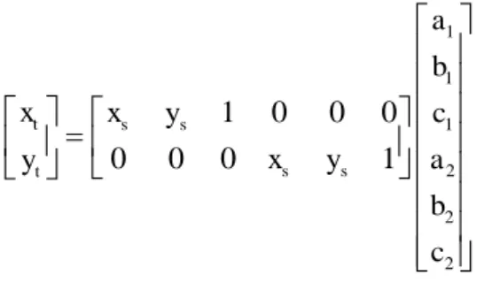
The mathematic model for the two-dimensional affine transformation is expressed as follows:
1
1
1
2
2
2
1 0 0 0
0 0 0 1
t s s
s s
t
a b
x x y c
x y a
y
b c
(22)
Table 1: Coordinates of points with random errors in start system and target system (unit: m)
coordinate 1 2 3 4 5 6 7 8 9 10
s
x
s
y
t
x
t
y
70.00 49.98 180.00
59.98
66.16 61.74 141.21 114.67
56.17 69.02 86.70 163.71
43.83 69.01 37.26 188.45
33.82 61.77 11.77 179.38
30.00 50.00 19.99 140.00
33.80 38.25 58.77 85.35
43.83 30.97 113.31
36.28
56.17 30.98 162.77
11.56
66.19 38.24 188.24
20.61
20
T
L X I h Ba
a a e
(23)
where a x y xs1, , , 1s s2 ys2 x10s ,y10s T,hT h h1T T2 h6T, 1 2 4 5
1 200, 0, , 0
T T T T
h h h h ,
3 1, 0,1, 0, ,1, 01 20 T
h , 6
1 20
0,1, 0,1, , 0,1
T
h , 1 1 2 2 10 10
1 20
, , , ,
T
t t t t t t
x y x y x y
L ,
1
2
6
B B B
B
, 1
20 20
1 0 0 0
0 0 0 0
1 0 0 0 0 0
B , 2
20 20
0 1 0 0
0 0 0 0
0 1 0 0 0 0
B , 3 6
20 20
0 0 0 0
0 0 0 0
0 0 0 0 0
B B
4
20 20
0 0 0 0
1 0 0 0
0 0 0 0 1 0
B , 5
20 20
0 0 0 0
0 1 0 0
0 0 0 0 0 1
B .
In order to give the reliable evaluations for the proposed outlier detection method, the following five schemes for adding outliers are discussed. The significant level for determining critical value is set as 0.05, which is very frequently used (Gao et al. 1992).
Scheme 1: According to Amiri-Simkooei and Jazaeri (2013), the outlier of magnitude 0.1 m which is 10 times of the priori standard deviation, is added into the xs component of point 4 in the start system.
The residuals of the observations and random vector a and the corresponding w-test statistics are displayed in Table 2. Obviously, the absolute values of residuals of thexcomponents of point 4 in the start system and target system are greater than others. Meanwhile, both wa27 4.6774and
7 3.7011 L
w surpass the threshold value u0.975 = 1.96. So we deem that there is an outlier in the
x component of the start system, target system or both, which is kept the same with the set simulated case. However, we can’t determinate the special position of the outlier.Scheme 2: The outlier of magnitude 0.1 m is added into both components of point 4 in the start system.The residuals and w-test statistics are shown in Table 3. As we know, the absolute values of residuals of the x components of point 4 in both coordinate systems are greater than others.Particularly,
both wa27 2.7943and wL7 3.2089for thexcomponent of point 4 are beyond the threshold
value1.96 , and wL8 2.8142for the yt component of point 4 in the target system exceeds 1.96
too. Although wa28 1.8708for the ys component of point 4 in the start system is smaller than
outliers.
Table 2: Residuals of observations and random vector a and corresponding w-test statistics (Scheme 1) (unit: m)
Point No.
Target system Start system
Coordinate VLj wLj Coordinate Vai wai
1 xt
t
y
-0.0013973 -0.00035329
-0.25266 -0.063881
s
x
s
y
0.0048841 -0.0013852
0.32287 -0.091561
2 xt
t
y
0.0091772 0.0053935
1.6594 0.97525
s
x
s
y
-0.025934 -0.025934
-1.7144 -0.21159
3 xt
t
y
0.008246 0.0015716
1.491 0.28417
s
x
s
y
-0.029849 0.010229
-1.9732 0.67613
4 xt
t
y
-0.020466
-0.0055651
-3.7011
-1.0064
s
x
s
y
0.070755
-0.018725
4.6774
-1.2377
5 xt
t
y
0.0046209 -0.0011276
0.83561 -0.20392
s
x
s
y
-0.020742 0.013769
-1.3712 0.91015
6 xt
t
y
0.0036126 0.0021386
0.65332 0.38674
s
x
s
y
-0.010178 -0.0013217
-0.67285 -0.087364
7 xt
t
y
0.0054174 0.0020203
0.97969 0.36536
s
x
s
y
-0.017635 0.0027668
-1.1658 0.18289
8 xt
t
y
-0.0040845 0.00026835
-0.7386 0.048526
s
x
s
y
0.016878 -0.0092558
1.1158 -0.61182
9 xt
t
y
0.00051964 -0.00050291
0.093964 -0.090939
s
x
s
y
-0.0030844 0.0030535
-0.2039 0.20184
10 xt
t
y
-0.0056462 -0.0038434
-1.021 -0.69502
s
x
s
y
0.014906 0.0040706
Table 3: Residuals of observations and random vector a and corresponding w-test statistics (Scheme 2) (unit: m)
Point No.
Target system Start system
Coordinate VLj wLj Coordinate Vai wai
1 xt
t
y
-0.00093979 0.00072597
-0.10477 0.080929
s
x
s
y
0.0052099 -0.0047832
0.22502 -0.20659
2 xt
t
y
0.011106 0.0099526
1.238 1.1094
s
x
s
y
-0.024541 -0.017565
-1.06 -0.75868
3 xt
t
y
0.011362 0.0089374
1.2665 0.99627
s
x
s
y
-0.024541 -0.017565
-1.1918 -0.56127
4 xt
t
y
-0.028779 -0.025239
-3.2089 -2.8142
s
x
s
y
0.064696 0.043314
2.7943 1.8708
5 xt
t
y
0.0077303 0.0062289
0.86182 0.69444
s
x
s
y
-0.018478 -0.0094334
-0.79809 -0.40745
6 xt
t
y
0.0055308 0.006682
0.61665 0.745
s
x
s
y
-0.0087742 -0.015647
-0.37897 -0.6758
7 xt
t
y
0.0058653 0.0030857
0.65393 0.34403
s
x
s
y
-0.017298 -0.00059882
-0.7471 -0.025864
8 xt
t
y
-0.0048241 -0.0014746
-0.5378 -0.16439
s
x
s
y
0.016352 -0.0037588
0.70624 -0.16235
9 xt
t
y
-0.00067131 -0.0033185
-0.074838 -0.36994
s
x
s
y
-0.0039448 0.011924
-0.17038 0.51502
10 xt
t
y
-0.0063798 -0.0055804
-0.71127 -0.62215
s
x
s
y
0.014371 0.0095432
0.62072 0.41219
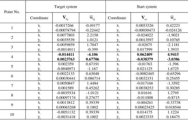
Scheme 3: The outlier of magnitude 0.1 m is added into the xscomponent of point 4 in the start system and the ytcomponent of point 4 in target system.
The residuals and the w-test statistics are obtained, which is displayed in Table 4. The results from Table 4 show that the test statistics satisfy wa27 4.9415>1.96and wL7 4.106>1.96, which
shows that the xcomponent of point 4 is possibly contaminated with an outlier. Although the absolute value of residual for the yt component of point 4 in the target system is small,
28 3.0386>1.96
a
Table 4: Residuals of observations and random vector a and corresponding w-test statistics (Scheme3) (unit: m)
Point No.
Target system Start system
Coordinate VLj wLj Coordinate Va i wai
1 xt
t y -0.0017266 -0.00078794 -0.49177 -0.22442 s x s y 0.0053326 -0.00030473 0.42223 -0.024126
2 xt
t y 0.0077803 0.0035539 2.2158 1.0121 s x s y -0.024022 0.0013597 -1.9021 0.10765
3 xt
t y 0.0059859 -0.0014011 1.7047 -0.399 s x s y -0.02675 0.017599 -2.1181 1.3933
4 xt
t y -0.014411 0.0023763 -4.106 0.67706 s x s y 0.062409 -0.038379 4.9415 -3.0386
5 xt
t y 0.002359 -0.0040971 0.67191 -1.167 s x s y -0.01763 0.021125 -1.396 1.6725
6 xt
t y 0.0022133 0.00030441 0.63048 0.086714 s x s y -0.0082465 0.0032151 -0.65296 0.25455
7 xt
t y 0.0050847 0.001589 1.4484 0.45262 s x s y -0.017166 0.0038252 -1.3592 0.30285
8 xt
t y -0.0035534 0.00097174 -1.0121 0.27677 s x s y 0.01616 -0.011008 1.2795 -0.8715
9 xt
t y 0.0013812 0.00063268 0.39339 0.1802 s x s y -0.004261 0.00023425 -0.33738 0.018546
10 xt
t y -0.0051132 -0.0031418 0.39339 0.1802 s x s y 0.014175 0.0023335 1.1224 0.18475
Table 5: Residuals of observations and random vector a and corresponding w-test statistics (Scheme 4) (unit: m)
Point No.
Target system Start system
Coordinate VLj wLj Coordinate Vai wai
1 xt
t y -0.0023489 -0.00016403 -0.58721 -0.041006 s x s y 0.0090658 -0.0040362 0.75905 -0.33795
2 x t
t y 0.0051497 0.00618 1.2873 1.5449 s x s y -0.0082485 -0.014416 -0.69062 -1.207
3 xt
t y 0.0017338 0.0028432 0.4334 0.71071 s x s y -0.0012538 -0.0079015 -0.10498 -0.6616
4 x t
t y -0.0030607 -0.008957 -0.76547 -2.2401 s x s y -0.0056531 0.029688 -0.47332 2.4858
5 xt
t y -0.0018874 0.00014316 -0.47184 0.035789 s x s y 0.0078336 -0.0043421 0.65589 -0.36357
6 xt
t y -0.00040699 0.0029242 -0.10176 0.73114 s x s y 0.0074691 -0.012501 0.62537 -1.0467
7 x t
t y 0.0044704 0.0021985 1.1177 0.54968 s x s y -0.013485 0.00014176 -1.1291 0.01187
8 xt
t y -0.0025448 -3.0876e-005 -0.63621 -0.0077191 s x s y 0.010115 -0.0049597 0.84692 -0.41528
9 x t
t y 0.0030058 -0.00099484 0.75143 -0.2487 s x s y -0.014008 0.0099803 -1.1728 0.83567
10 xt
Table 6: Residuals of observations and random vector a and corresponding w-test statistics with deleting point 4 in both of start system and target system (unit: m)
Point No.
Target system Start system
Coordinate VLj wLj Coordinate Vai wai
1 xt
t y -0.0025167 -0.00065539 -0.7071 -0.18414 s x s y 0.0087558 -0.0024088 0.89974 -0.24753
2 xt
t y 0.0044403 0.0041034 1.2804 1.1833 s x s y -0.0095588 -0.0075354 -0.98226 -0.77434
3 xt
t y 0.0005872 -0.00051201 0.17764 -0.15489 s x s y -0.0033716 0.0032211 -0.34646 0.331
4 xt
t y - - - - s x s y - - - -
5 xt
t y -0.0030325 -0.0032077 -0.91736 -0.97033 s x s y 0.0057185 0.0067668 0.58763 0.69537
6 xt
t y -0.0011139 0.00085512 -0.3212 0.24659 s x s y 0.0061635 -0.0056457 0.63336 -0.58015
7 xt
t y 0.0043048 0.0017142 1.2096 0.48168 s x s y -0.013791 0.001748 -1.4172 0.17963
8 xt
t y -0.002273 0.00076394 -0.64022 0.21517 s x s y 0.010617 -0.0075976 1.091 -0.78073
9 xt
t y 0.0034443 0.00028881 0.97631 0.081865 s x s y -0.013198 0.0057284 -1.3562 0.58866
10 xt
t y -0.0038405 -0.0033504 -1.0817 -0.94369 s x s y 0.0086644 0.0057231 0.89036 0.58811
Table 7: Residuals of observations and random vector a and corresponding w-test statistics (Scheme 5) (unit: m)
Point No.
Target system Start system
Coordinate VLj wLj Coordinate Vai wai
1 xt
t y 0.0045553 0.0018727 0.82093 0.33749 s x s y -0.014464 0.0016235 -0.88826 0.09968
2 xt
t y -0.016465 -0.0067103 -2.9676 -1.2095 s x s y 0.052397 -0.0061015 3.2177 -0.37462
3 xt
t y 0.0059838 -0.0014032 1.0783 -0.25286 s x s y -0.026717 0.017593 -1.6407 1.0802
4 xt
t y 0.0098111 0.012636 1.7687 2.2779 s x s y -0.013972 -0.03093 -0.85803 -1.8991
5 xt
t y -0.0039266 -0.0067598 -0.70769 -1.2183 s x s y 0.0021913 0.019193 0.13456 1.1784
6 xt
t y -0.0040698 -0.002357 -0.73355 -0.42483 s x s y 0.011557 0.0012864 0.70971 0.078982
7 xt
t y 0.0012096 -5.41e-005 0.21801 -0.0097511 s x s y -0.004942 0.0026377 -0.30348 0.16195
8 xt
t y -0.0035487 0.00097413 -0.63958 0.17556 s x s y 0.016128 -0.011002 0.9904 -0.67549
9 xt
t y 0.0052762 0.0022808 0.9509 0.41105 s x s y -0.016531 0.0014335 -1.0151 0.088012
10 xt
Scheme 4: The outlier of magnitude 0.1m is added into the ycomponent of point 4 in both start system and target system.
The concrete results are presented in Table 5. It is not difficult to know wa28 2.4858>1.96 andwL8 2.2401>1.96from Table 5, but the absolute values of other w-statistics are smaller than
1.96. It means that only ycomponent of point 4 contains an outlier, which is consistent with the set simulated case. If we will delete point 4 in both coordinate systems, the new results about the residuals and w-test statistics are obtained, which is displayed in Table 6. It is shown that all wai
and wLj are smaller than the threshold value 1.96, which demonstrates that the remaining
observations are clean without the effects of outliers.
We just discuss the case that the outlier locates in the same point in two different systems for scheme 1 to 4. In fact, there may be multiple outliers in the different points for the two-dimensional coordinate transformation. Hence, the following scheme 5 is used to assess the efficiency of the proposed procedure for detecting multiple outliers in the partial EIV model.
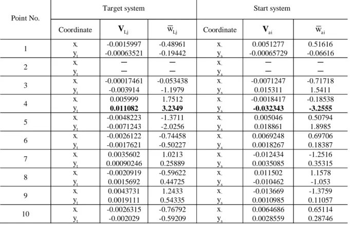
Scheme 5: In this simulation, two outliers of magnitude 0.1 m are added to the xscomponent of point 2 in the start system and the yt component of point 4 in the target system, respectively.
The detail results about the residuals and w-test statistics are listed in Table 7. wa23 3.2177>1.96
and wL3 2.9676>1.96 indicate thatthe xcomponent of point 2 contains an outlier. On the other
hand, due towa28 1.8991andwL8 2.2779>1.96, the ycomponent of point 4 is probable to be
Table 8: Residuals of observations and random vector a and corresponding w-test statistics with deleting the point 2 in both of start system and target system (Scheme 5) (unit: m)
Point No.
Target system Start system
Coordinate VLj wLj Coordinate Vai wai
1 xt
t y -0.0015997 -0.00063521 -0.48961 -0.19442 s x s y 0.0051277 -0.00065729 0.51616 -0.06616
2 xt
t y - - - - s x s y - - - -
3 xt
t y -0.00017461 -0.003914 -0.053438 -1.1979 s x s y -0.0071247 0.015311 -0.71718 1.5411
4 xt
t y 0.005999 0.011082 1.7512 3.2349 s x s y -0.0018417 -0.032343 -0.18538 -3.2555
5 xt
t y -0.0048223 -0.0071243 -1.3711 -2.0256 s x s y 0.005046 0.018861 0.50794 1.8985
6 xt
t y -0.0026122 -0.0017621 -0.74458 -0.50227 s x s y 0.0069248 0.0018267 0.69706 0.18387
7 xt
t y 0.0035602 0.00090246 1.0213 0.25889 s x s y -0.012434 0.0035085 -1.2516 0.35315
8 xt
t y -0.0020919 0.0015692 -0.59622 0.44725 s x s y 0.011502 -0.010462 1.1578 -1.053
9 xt
t y 0.0043731 0.0019111 1.2433 0.54335 s x s y -0.013669 0.0010985 -1.3759 0.11057
10 xt
t y -0.0026315 -0.002029 -0.76792 -0.59209 s x s y 0.0064686 0.0028559 0.65114 0.28746
Table 9: Residuals of observations and random vector a and corresponding w-test statistics with deleting point 2 and point 4 in both of start system and target system (Scheme 5) (unit: m)
Point No.
Target system Start system
Coordinate VLj wLj Coordinate Vai wai
1 xt
t y -0.00070383 0.00102 -0.23467 0.34007 s x s y 0.004853 -0.0054855 0.58449 -0.66066
2 xt
t y - - - - s x s y - - - -
3 xt
t y 0.0027479 0.0014848 1.0525 0.56868 s x s y -0.0080217 -0.00044471 -0.96613 -0.053561
4 xt
t y - - - - s x s y - - - -
5 xt
t y -0.002371 -0.0025964 -0.79065 -0.8658 s x s y 0.0042931 0.0056432 0.51706 0.67966
6 xt
t y -0.0012774 0.00070397 -0.40134 0.22118 s x s y 0.0065153 -0.0053684 0.7847 -0.64656
7 xt
t y 0.0036943 0.0011501 1.1405 0.35506 s x s y -0.012475 0.0027853 -1.5025 0.33546
8 xt
t y -0.0027834 0.00029229 -0.85898 0.090205 s x s y 0.011715 -0.0067323 1.4109 -0.81083
9 xt
t y 0.0035459 0.00038276 1.0946 0.11816 s x s y -0.013415 0.005557 -1.6157 0.66929
10 xt
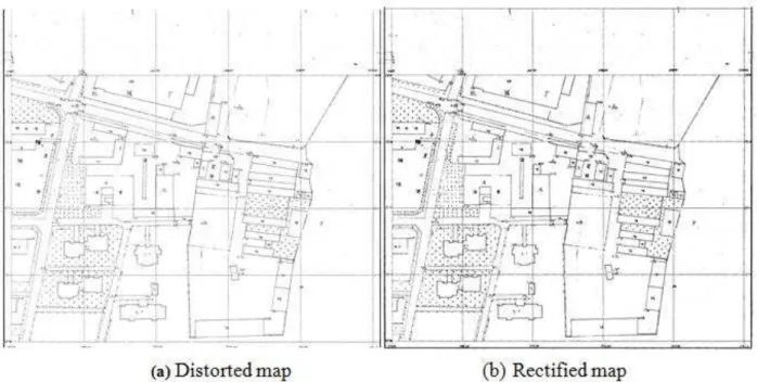
4.2 Real data about map rectification
The example is about the map rectification. The 2D affine transformation is used to rectify the map. The scale of map is 1:500 for figure 1.
Figure 1: The distorted map and its rectified map using affine transformation
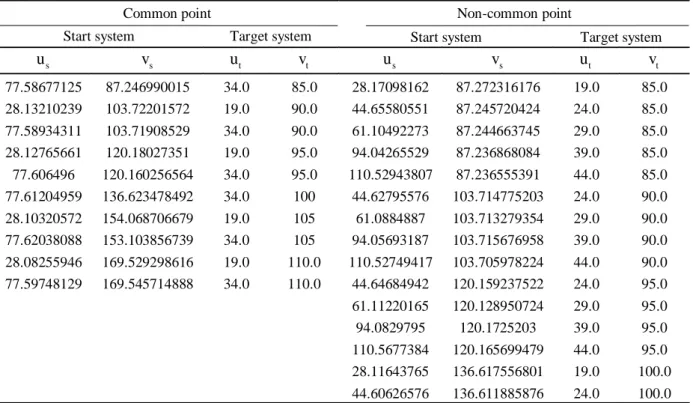
There are ten common points whose theoretical coordinates are previously known, and then we sample their coordinates on the distorted map. The affine transformation is used to rectify the map. The sampled coordinates and theoretical coordinates of common points are treated as the coordinates in the start system and target system, respectively, which is displayed in Table 10. The transformation parameters can be estimated by using the common points with the 2D affine transformation. By employing the proposed algorithm, the residuals and w-test statistics of the observations and random vector aare derived, which is shown in Table 11. Because the w-test statistics satisfy wL14 21.838>1.96and wa34 21.172>1.96, the point 7 is suspected as an
outlier and should be deleted. Then the new residuals and w-test statistics are obtained, which can be found in Table 12. Due to wa35 1.7622<1.96for point 9 in the target system, there are no
outliers in the observations even if wL15 2.297>1.96according to the criterion for identifying
Table 10: Coordinates of ten common points and fifteen non-common points in both coordinate systems (unit: cm)
Common point Non-common point
Start system Target system Start system Target system
s
u vs ut vt us vs ut vt
77.58677125 28.13210239 77.58934311 28.12765661 77.606496 77.61204959 28.10320572 77.62038088 28.08255946 77.59748129 87.246990015 103.72201572 103.71908529 120.18027351 120.160256564 136.623478492 154.068706679 153.103856739 169.529298616 169.545714888 34.0 19.0 34.0 19.0 34.0 34.0 19.0 34.0 19.0 34.0 85.0 90.0 90.0 95.0 95.0 100 105 105 110.0 110.0 28.17098162 44.65580551 61.10492273 94.04265529 110.52943807 44.62795576 61.0884887 94.05693187 110.52749417 44.64684942 61.11220165 94.0829795 110.5677384 28.11643765 44.60626576 87.272316176 87.245720424 87.244663745 87.236868084 87.236555391 103.714775203 103.713279354 103.715676958 103.705978224 120.159237522 120.128950724 120.1725203 120.165699479 136.617556801 136.611885876 19.0 24.0 29.0 39.0 44.0 24.0 29.0 39.0 44.0 24.0 29.0 39.0 44.0 19.0 24.0 85.0 85.0 85.0 85.0 85.0 90.0 90.0 90.0 90.0 95.0 95.0 95.0 95.0 100.0 100.0
Table 11: Residuals of observation and random vector a and corresponding w-test statistics for mapping rectification (unit: cm)
Point No.
Target system Start system
Coordinate VLj wLj Coordinate Vai wai
1 xt
t y 0.0054641 -0.02307 0.66522 -2.8086 s x s y -0.0016239 0.006993 -0.58441 2.5164
2 xt
t y -0.0048054 0.045573 -0.58676 5.5647 s x s y 0.0013928 -0.013814 0.50126 -4.971
3 xt
t y 0.0042668 -0.016875 0.4667 -1.8457 s x s y -0.0012697 0.0051151 -0.45693 1.8406
4 xt
t y -0.0040557 0.055618 -0.45558 6.2476 s x s y 0.0011516 -0.016859 0.41444 -6.0667
5 xt
t y -0.00098049 -0.0021115 -0.10244 -0.22059 s x s y 0.00030013 0.00064008 0.10801 0.23033
6 xt
t y -0.0030061 0.0065435 -0.31407 0.68363 s x s y 0.000902 -0.0019835 0.32462 -0.71373
7 xt
t y 0.0018414 -0.1941 0.20717 -21.838 s x s y -0.00028704 0.058838 -0.1033 21.172
8 xt
t y -0.0058015 0.010432 -0.63472 1.1414 s x s y 0.0017438 -0.0031622 0.62757 -1.1379
9 xt
t y 0.0070075 0.092938 0.85308 11.314 s x s y -0.0022537 -0.028173 -0.81107 -10.138
10 xt
Table 12: Residuals of observation and random vector a and corresponding w-test statistics for mapping rectification with deleting point 7 (unit: cm)
Point No.
Target system Start system
Coordinate VLj wLj Coordinate Vai wai
1 xt
t y
0.005221 0.0026575
1.3414 0.68277
s x
s y
-0.0015825 -0.00080753
-1.1719 -0.59671
2 xt
t y
-0.0043552 -0.0019646
-1.1521 -0.51971
s x
s y
0.0013201 0.00059699
0.97753 0.44113
3 xt
t y
0.0041199 -0.0014459
0.94397 -0.33129
s x
s y
-0.0012487 0.00043918
0.97753 0.44113
4 xt
t y
-0.0035079 -0.0022192
-0.86199 -0.54533
s x
s y
0.0010633 0.00067433
0.78736 0.49828
5 xt
t y
-0.0010283 0.0030519
-0.22444 0.6661
s x
s y
0.00031166 -0.00092718
0.23079 -0.68512
6 xt
t y
-0.002957 0.0014165
-0.64539 0.30916
s x
s y
0.00089626 -0.00043027
0.66369 -0.31794
7 xt
t y
- -
- -
s x
s y
- -
- -
8 xt
t y
-0.0056571 -0.0049908
-1.2965 -1.1438
s x
s y
0.0017147 0.0015164
1.2698 1.1205
9 xt
t y
0.0078511 0.0041787
2.297 1.2226
s x
s y
-0.0023797 -0.0012697
-1.7622 -0.93825
10 xt
t y
0.00031337 -0.00068396
0.080512 -0.17573
s x
s y
-9.4978e-005 0.00020779
-0.070332 0.15354
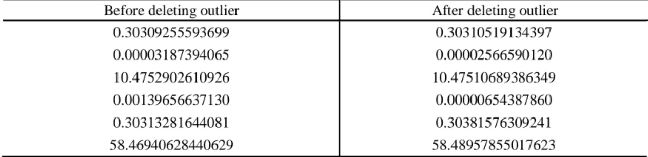
Table 13: Transformation parameters estimated by the WTLS method before deleting outlier and after deleting outlier (unit: cm)
Before deleting outlier After deleting outlier
0.30309255593699
0.00003187394065
10.4752902610926 0.00139656637130
0.30313281644081 58.46940628440629
0.30310519134397
0.00002566590120
10.47510689386349 0.00000654387860
0.30381576309241 58.48957855017623
5. CONCLUSIONS
two-dimensional affine transformation, the identification of outliers is implemented only once through the proposed procedure compared with previously approach while single outlier is considered. For multiple outliers, the repeated test with step by step is suggested. However, we still can’t discriminate that the outliers locate in the observation or coefficient matrix or both, which is a very open problem to be discussed in the future.
ACKNOWLEDGEMENTS
The authors are grateful to the editor and two anonymous reviewers for their constructive comments and suggestions so that the paper is substantial improved. This research has been supported jointly by the National Natural Science Foundation of China (Grant No. 41174005, 414714009) and State Key Laboratory of Geodesy and Earth’s Dynamics (SKLGED 2017-3-2-E)
REFERENCES
Akyilmaz, O. “Total least squares solution of coordinate transformation.”Survey Review 39 (303) (2007): 68-80.
Amiri-Simkooei, A.R. and Jazaeri, S. “Data-snooping procedure applied to errors-in-variable models.”Stud.Geophys.Geod. 57 (2013): 426-441.
Amiri-Simkooei, A.R. and Jazaeri, S. “Weighted total least-squares formulated by standard least-squares theory.” Journal of Geodetic Science 2(2) (2012): 113-124.
Baarda, W. “A testing procedure for use in geodetic networks.” Pubications on Geodesy 2(5) (1968), Netherlands Geodetic Commission, Delft, the Newtherlands.
Baselga, S. “Critical limitation in use of test for gross error detection.” Jounral of Surveying Engineering 133(2) (2007): 52-55.
Fang, X. “A total least squares solution for geodetic datum transformations.” Acta Geod Geophys 49 (2014): 189-207.
Fang, X. “Weighted total least squares: necessary and sufficient conditions, fixed and random parameters.”Journal of Geodesy 87 (2013): 733-749.
Gao, Y., Krakiwsky, E.J. and Czompo J. “Robust testing procedure for detection of multiple blunders.”Journal of Surveying Engineering 118 (1992): 11-23.
Gloub, G.H. and Van Loan, C. F. “An analysis of the total least squares problem.” SIAM J. Numer. Anal. 17(6) (1980): 883-893.
Gui, Q.M. and Liu, J.S. “Generalized shrunken-type robust estimation.” Jounral of Surveying Engineering 125(4) (1999):177-184.
Gui, Q.M., Gong, Y.S., Li, G.Z. and Li, B.L. “A Bayesian approach to the detection of gross errors based on posterior probability.” Journal of Geodesy 81(2007): 651-659.
Gui, Q.M., Li G.Z., and Ou J.K. “Robust-biased estimation based on quasi-accurate detection.”
Gui, Q.M., Li G.Z., and Ou J.K. “Robust-Type Biased Estimation in Gauss-Markov Model.”
Survey Review 38(298) (2005b): 299-307.
Gui, Q.M., Li, X., Gong, Y.S., Li, B.L. and Li, G.Z. “Bayesian unmasking method for locating multiple gross errors based on posterior probabilities of classification variables.” Journal of Geodesy 85 (2011): 191-203.
Guo, J.F. and Zhao, J. “Comparative analysis of statistical tests used for detection and identification of outliers (in Chinese).” Acta Geodaetica et Cartographica Sinica 41(1) (2012): 14-18.
Guo, J.F., Ou, J.K. and Wang, H.T. “Quasi-accurate detection of outliers for correlated observations.”Journal of Surveying Engineering 133 (2007): 129-133.
Hekimoglu, S. and Erenoglu, R.C. “New method for outlier diagnostics in linear regression.”
Journal of Surveying Engineering 135(3) (2009): 85-89.
Hekimoglu, S. “Do robust methods identify outliers more reliably than conventional tests for outliers?”ZFV 130 (2005): 174-180.
Hekimoglu, S., Erdogan, B., Soycan, M. and Durdag, U.M. “Univariate approach for detecting outliers in geodetic networks.”Journal of Surveying Engineering 140 (2014): 1-8.
Huber, P.J. Robust Statistics. New York: John Wiley & Sons, 1981.
Jazaeri, S., Amiri-Simkooei, A.R. and Sharifi, M.A. “Iterative algorithm for weighted total least squares adjustment.”Survey Review 46(334) (2014): 19-27.
Koch, K.R. “Parameter Estimation and Hypothesis Testing in Linear Models, 2nd Edition.” Berlin: Springer-Verlag, Berlin, 1999.
Kok, J.J. “On data snooping and multiple outliers testing.” Rochville: NOAA Technical Report, Nos NGS 30, 1984.
Lehmann, R. “On the formulation of the alternative hypothesis for geodetic outlier detection.”
Journal of Geodesy 87 (2013): 373-386.
Li, B.F., Shen Y.Z., Zhang X.F., Li C. and Lou L.Z. “Seamless multivariate affine error-in-variables transformation and its application to map rectification.”International Journal of Geographical Information Science 27(8) (2012): 1572-1592.
Li, B.F., Shen, Y.Z. and Lou, L.Z. “Noniterative datum transformation revisited with two-dimensional affine model as a case study.” Journal of Surveying Engineering 139 (2013): 166-175.
Mahboub, V. “On weighted total least-squares for geodetic transformations.”Journal of Geodesy
86 (2012): 359-367.
Pope, A.J. “The statistics of residuals and the detection of outliers.” Rochville: NOAA Technical report, Nos 65, NGS 1, 1976.
Rousseeuw, P.J. and Leroy, A.M. “Robust Regression and Outliers Detection.” New York: John Wiley & Sons, 1987.
Schaffrin, B. and Uzun, S. “Errors-in-variables for mobile algorithms in the presence of outliers.”Archives of Photogrammetry, Cartograhy and Remote Sensing 22 (2011): 377-387.
Schaffrin, B. and Uzun, S. On the reliability of errors-in-variables models. Acta Et Commentationes Universitatis Tartuensis De Mathematica 16(1) (2012): 69-81.
Schaffrin, B. and Wieser, A. “On weighted total least-squares adjustment for linear regression.”
Journal of Geodesy 82 (2008): 415-421.
Shen, Y.Z., Li, B.F. and Chen, Y. “An iterative solution of weighted total least-squares adjustment.”Journal of Geodesy 85 (2011): 229-238.
Xu, P.L., Liu, J.N. and Shi, C. “Total least-squares adjustment in partial errors-in-variables models: algorithm and statistical analysis.”Journal of Geodesy 86 (2012): 661-675.