A Work Project, presented as part of the requirements for the Award of a Master Degree in Finance from the NOVA – School of Business and Economics.
OPTIMAL CONCENTRATION FOR VALUE AND MOMENTUM
PORTFOLIOS
LEONOR MARIA DE SANTA MARTA GRANGER BAPTISTA
STUDENT 2291
A Project carried out on the Master in Finance Program, under the supervision of:
Professor Fernando Anjos
Optimal Concentration for Value and Momentum Portfolios
Abstract
This paper aims to verify the persistence of the profitability of the Momentum strategy, first
implemented by Richard Driehaus in the 1980’s. Furthermore, the paper will test the impact
of changing several parameters of the strategy on its profitability. A combination of the
Momentum strategy with a Value-oriented one will also be analyzed, with a view to assess
the outperformance of this aggregate portfolio. The results are in line with Jedadeesh and
Titman (2001), there is still evidence for its profitability in recent years, except in times of
severe volatility. Additionally, there is an improvement in combining the two strategies.
I. Introduction
The main purpose of this paper is the continuation of the study of Jegadeesh and
Titman (1993, 2001) on the Momentum strategy, whose results challenge the widely accepted
market efficiency theory, established in 1969 by Eugene Fama (Efficient Market Hypothesis).
In this light, the Momentum strategy shouldn’t be profitable because it states that it’s
impossible to continuously beat the market given that all the relevant information is already
reflected in stock prices. In theory, investors should make informed decisions, and having
access to the information on this strategy and its profitability, enough individuals should be
investing in it causing its abnormal returns to disappear.
With that as a starting point, I extended the analysis period up until 2015 and
additionally designed and tested several variations to the zero-cost Momentum portfolio.
Namely, tests were done for portfolios with different number of companies and different
holding periods, as well as different ranking periods and lags. The objective being to analyze
the possible impact that these parameters may have and optimize the strategy. Lastly, an
analysis was done for a combination of the Momentum strategy with a Value-oriented
strategy, maintaining a zero-cost portfolio, with the purpose of testing whether this new
portfolio would result in a larger Sharpe Ratio than the stand-alones, expected due to their
individual profitability and the anticipated uncorrelation between the two, which would
increase diversity and so decrease volatility.
This paper will start with a literature review of the historical progress and studies of
both Momentum and Value strategies, afterwards it will continue with the development of the
hypothesis to be tested and the methodology used. The results and discussions will be
and combination of both strategies. The two final sections will be for the limitations to the
paper and the conclusion. A more detailed reference list can be found at the end.
II. Literature Review
Momentum is an investment strategy that consists in buying the best performing
companies, and shorting the worst performers. The idea behind it is in line with the saying of
“the trend is your friend”, which means that you expect that the companies will continue to
follow the path that they’ve been having in the short-term. To follow this strategy, an
investor needs to choose which group of stocks he will consider. For example, if his choice
fell on the American stock market, he then would need to choose the number of companies in
wish to invest, the number of months relevant for the ranking of the companies and the
holding period. Also, he must determine if he would like to have a lag. A lag is when he waits
two weeks or a month for example before investing, and this is often done due to short-term
return reversals, which is when a company inverts its current path in the very short-term
(under one month) as shown in de Groot et al (2011).
The Momentum strategy can be traced back to the 1950’s with Richard Donchian’s
innovative trend following ideas. His strategy was used for commodity trading and it involved
using moving averages and investing based on the higher and lower values. However, more
commonly, Richard Driehaus is considered to be the father of the strategy, since in the 1980’s
he implemented it to run his funds. His idea was against Wall Street’s practice at the time, of
“buy low, sell high”, he instead followed the concept of “buy high, sell higher”. Since then,
there have been many papers that attempt to explain and recreate this strategy, in Jegadeesh
and Titman in 1993 and 2001, in Asness et al (2013), Daniel Moskowitz (2015) and many
others. The reason why this strategy persists is still under discussion; the two better accepted
tendencies, see Jegadeesh and Titman (2001) for more discussion on the several explanations.
However, all of them agree that it has statistically significant abnormal returns in periods
between 1945 and 2015.
A more recent variation of this strategy is the Alpha Momentum, which was first
documented in Grundy and Martin (1998). This new strategy came as a way of improving the
Standard Momentum, by increasing its returns and decreasing its volatility, as was
demonstrated in Hühn and Scholz (2013). In this strategy, the variable used to rank the
companies is no longer past returns, but instead it’s the alpha that represents the abnormal
return and can be calculated with models such as the CAPM (Capital Asset Pricing Model),
the Fama-French three-factor, or the Fama-French-Carhart four-factor model, represented in
Equations I, II and III, respectively.
The CAPM model was developed by Sharpe (1964) and Lintner (1965), and its
purpose was to establish a connection between a company’s returns and the market. The
tested hypothesis was that the returns would equal the risk-free rate plus a coefficient of the
market’s excess return (MKTRF stands for Market minus Risk Free). This coefficient could
be positive if the company had a positive correlation with the market’s excess return, or
negative otherwise. Currently, it is more common to assume that the returns of a company are
equal to an abnormal return plus the risk-free rate, plus the coefficient of the market’s excess
return. This abnormal return, commonly referenced as alpha, will be the indicator used for the
Alpha Momentum in this paper. The CAPM, despite being questioned in papers such as Black
(1972), which state that the market’s excess return is not the only relevant factor, is still
widely used for its simplicity.
Equation I – CAPM Alpha (Jensen’s Alpha)
𝛼
! =𝑟!− [𝑟!+𝛽!𝑀𝐾𝑇𝑅𝐹+𝜀]
The Fama-French three-factor Model came as an extension to the CAPM, and was
returns, but with more descriptive variables to improve the model’s explanatory power.
Besides using the market’s excess return as factor, it adds a size and a value element, written
in Equation II as SMB (Small-Minus-Big) and HML (High-Minus-Low), respectively. The
size factor represents the difference in returns between firms with small and large Market
Capitalizations, since smaller firms have historically outperformed bigger firms. The value
factor represents the difference in returns between value firms and growth firms, since,
following the same reasoning, historically firms with high book-to-market ratios, value firms,
have outperformed firms with low book-to-market ratios, growth firms.
Equation II – Fama-French three-factor Alpha
𝛼! =𝑟!−[𝑟!+𝛽!"#$%𝑀𝐾𝑇𝑅𝐹+𝛽!"#𝑆𝑀𝐵+𝛽!!"𝐻𝑀𝐿+𝜀]
The Fama-French-Carhart 4-factor model developed by Carhart (1997) adds another
element, a Momentum factor written in Equation III as UMD (Up-Minus-Down), and
represents the difference in returns between companies with previously high returns and
companies with previously low returns, commonly referred to as winners minus losers.
Equation III – Fama-French-Carhart four-factor Alpha
𝛼! =𝑟!−[𝑟!+𝛽!"#$%𝑀𝐾𝑇𝑅𝐹+𝛽!"#𝑆𝑀𝐵+𝛽!!"𝐻𝑀𝐿+𝛽!"#𝑈𝑀𝐷+𝜀]
Besides analyzing the optimal concentration of Momentum portfolios, I will also
study combination portfolios that include Value stocks.A portfolio of Value stocks is built by
buying the companies that are undervalued with the expectation that the market will correct
this undervaluation and the price will rise, and short the companies that are overvalued
following the same logic. Benjamin Graham and David Dodd first established it in 1928 while
teaching in Columbia Business School, resulting in the publication of their book Security
Analysis in 1934. Following the approach of several papers that studied this strategy, such as
Asness et al (2013), I use the ratio of price-to-book to understand whether there is some
overvaluation or undervaluation of a company in a point in time. I use this variable because,
has also been done with other accounting ratios such as Price-to-Earnings, for example in
Truong (2009).
As a comparison and evaluation measure of the different portfolios, I will use the ratio
developed by Sharpe (1966), known as Sharpe Ratio, since it takes into account both the
excess return when comparing to the risk-free rate and the volatility.
Equation IV – Sharpe Ratio
𝑆ℎ𝑎𝑟𝑝𝑒𝑅𝑎𝑡𝑖𝑜= 𝑟!−𝑟! 𝜎!
III. Hypothesis Development:
What I propose to do can be divided in three main goals. Firstly I want to expand the
study of the Momentum strategy to the end of 2015, to study if the abnormal returns found in
Jagadeesh and Titman (1993, 2001) until 1998 are still observable. Secondly, I want to
calibrate the model, by varying four parameters of the strategy and finding their optimal
values. The chosen parameters are: ranking period, lag before investing, holding period and
number of companies to invest in. For this, I will analyze both a Standard Momentum and the
Alpha Momentum, being that for the latter I will use the CAPM Model’s alpha as the ranking
variable.
The range of values for those parameters are based on other papers on the Momentum
strategy, for example, Jegadeesh and Titman (2001) use a six-months ranking period. Also
very important is the choice of stock exchanges, which this paper follows studies such as
Jegadeesh and Titman (2001) and Fisher et al (2016), which use all stocks in the NYSE,
AMEX and NASDAQ stock exchanges.
Finally, I want to analyze whether an investor would benefit from combining a
Standard Momentum strategy with a Value strategy, using the price-to-book accounting ratio
For all the strategies previously mentioned, all portfolios will have an equally
weighted long and short component, with an equal number of firms in each. As consequence,
all portfolios will be zero-cost, a long-short dollar-neutral strategy. During this paper, all
variables (returns, standard deviations, Sharpe Ratios) have been annualized unless specified
otherwise.
I expect to find that the strategy is still profitable, although this might happen at a
lower level due to the widening awareness of its existence. When combining it with a Value
strategy, I expect that they will be uncorrelated and if this happens then there might be
benefits of combining the two at least in terms of a lower volatility, and if large enough this
should compensate the expected drop in returns due to the expectation that the Value strategy
will yield lower returns, result found in Fisher et al (2016), and lead to a higher Sharpe Ratio.
Additionally, for the Standard Momentum strategy, I aim to choose the best variation
when considering the parameters described previously. When combining it with the Value
strategy, I also aim to choose the best concentration in terms of how many companies to
invest in, while always maintaining an equal weight between both strategies. The reason why
we expect there to be an optimal concentration level and not a monotonic increase/decrease of
Sharpe Ratio is because it is expected that both the Momentum’s returns and risk will
decrease with an increase in diversification, and we aim to find the best values for this
trade-off. Another reason for there to be an optimal concentration is due to transaction costs, which
increase with the increase of diversification, and so it can offset a rise in returns if it’s not
large enough. This paper doesn’t formally address transaction costs, however a consideration
is made to them in the Limitations section.
Throughout this paper, references to the number of companies always pertain to one
leg of the strategy. For example, a point in a graph representing a Sharpe Ratio for a strategy
short, and if this happens for the combination of strategies, it means 100 companies long and
100 companies short on both portfolios.
IV. Methodology:
In general terms, there were three steps that I followed in order to get the final results:
firstly I downloaded the data from Wharton University of Pennsylvania’s database WRDS
(“The Global Standard for Business Research”); secondly, using the programming software
Matlab (Matrix Laboratory), I processed and cleaned the data; lastly, using the same software,
I created an algorithm to implement the strategy.
More specifically, the data downloaded was for all stocks in the NYSE, NASDAQ and
AMEX, which consisted of around 30,000 stocks, from 1965 until the end of 2015. To control
for survivorship bias, companies that leave the stock exchange are still considered. The data
needed for each stock is the entry and exit from its respective stock exchange, its monthly
price and monthly number of shares outstanding to calculate its monthly Market
Capitalization, and monthly price to book ratios. The daily data needed was its holding period
return, which accounts for events such as stock splits and dividends, and resulted in a total of
80 million data points. To identify the stocks I used the database’s unique identifier, called the
PERMNO, since it doesn’t change with time for any given company, contrary to the Ticker or
Company Name, which may and frequently do change. Other data needed was the risk-free
rate, the market return, small-minus-big factor, high-minus-low factor and up minus down
factor, all available in the same database.
The data processing was a relatively complex part and very work-intensive, as often is
the case when the data to handle is large. Firstly I organized and cleaned the data: for
example, concerning the daily returns, if the company had no return information, it was
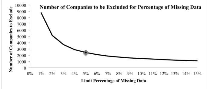
values, or “holes”, it was also removed. For this purpose I used 5% as reference, so only
companies with less than 5% missing returns were considered. For the model to work, the
missing returns had to be replaced, which I did, in each occurrence, with the minimum
between zero and the average of the closest previous and following return available, to be
conservative. I chose to use this value as reference because it seems to give a good trade-off
between the benefit of accuracy and loss in sample size, as can be seen in Figure I, a lower
percentage would result in more accuracy but would lead to an exponential decrease in the
number of companies considered.
Figure I - Number of Companies to be excluded for Percentage of Missing Data
After processing the data, I calculated the weekly returns from the daily if all returns
for that week are available; if not available, that week is not considered in the model for that
company. I used the same process to calculate the risk free, market, SMB, HML and UMD.
Finally, having all data necessary, I calculated the results for three different strategies:
the Standard Momentum, the Alpha Momentum, and finally a Value strategy. The idea
behind all three is similar, although in the first two I use only firms with a Market Cap higher
than 100million USD and in the third I change this limit to 1million USD instead. Optimally,
they should both have a lower limit of 200million to exclude penny stocks, which have
historically displayed a higher volatility and lower liquidity, studied in Liu et at (2011).
0 1000 2000 3000 4000 5000 6000 7000 8000 9000 10000
0% 1% 2% 3% 4% 5% 6% 7% 8% 9% 10% 11% 12% 13% 14% 15%
N
u
mb
er
of C
omp
an
ie
s to Exc
lu
d
e
Limit Percentage of Missing Data
However, this couldn’t be done due to the lack of sufficient data that fits this criterion.
Afterwards, I ranked the companies based on a chosen indicator (described below) from the
selected past months (the ranking period) and chose the top and bottom companies, then after
a lag, I calculated the return as if I had taken long/short positions on the chosen companies,
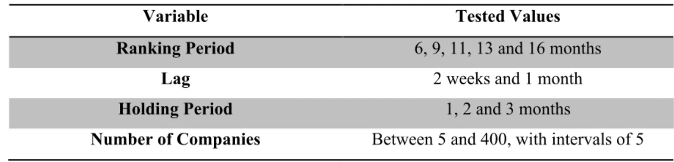
and then held that portfolio for the holding period. I tested this strategy for all combination of
variables in Table I:
Table I – Combination of different parameters to be tested in Momentum strategy
Variable Tested Values
Ranking Period 6, 9, 11, 13 and 16 months
Lag 2 weeks and 1 month
Holding Period 1, 2 and 3 months
Number of Companies Between 5 and 400, with intervals of 5
The chosen indicator is a function of the type of strategy: the Standard Momentum
strategy uses as indicator the cumulative return of the ranking period; the Alpha Momentum
uses the Jensen’s alpha obtained by regressing the weekly excess returns with the market
excess return for the ranking period; and finally the third uses the last price-to-book ratio
available of the ranking period.
As said before, the purpose of changing so many variables was to optimize the
calibration of the model. For each of them I calculate an average return, the standard
deviation, and the Sharpe Ratio. The combination shown below had the highest overall
Sharpe Ratio:
Base Strategy: Ranking Period – 11; Lag – 1; Holding Period – 3
As can be seen in Figure II, this strategy has an overall outperformance except for
highly concentrated portfolios, in which case it competes with a variant that only differs in the
month had very similar results, and so it is not included in Figure II but can be found in
Figure IV.B in the Annexes.
For the rest of this paper, this optimal strategy will be considered the Base Strategy
due to its overall outperformance.
Figure II - Sharpe Ratio of different variations of Momentum strategy per number of companies to invest in
V. Results
i. Momentum’s Profitability Over Time
In this section I wanted to study the abnormal returns of the Momentum strategy in
different periods, and for that purpose I used Jensen’s alpha from the CAPM model. Firstly,
the test for the entire period of 1965 to 2015 resulted in a statistically significant abnormal
return. Additionally, both tests for the periods of Jegadeesh and Titman’s papers, 1965 to
1989 and 1990 to 1998 (paper of 1993 and 2001, respectively), also proved significantly
greater than zero, which is what was expected, since in both papers they arrived at the same
conclusion. However, the strategy for the period of 1999 to 2015 does not yield a statistically
significant abnormal return. As this result was not expected, I split this period into sub periods
to study it in more detail, and found that within this period occurred two financial crisis, in
0.00 0.10 0.20 0.30 0.40 0.50 0.60 0.70 0.80 0.90 1.00
5
20 35 50 65 80 95 110 125 140 155 170 185 200 215 230 245 260 275 290 305 320 335 350 365 380 395
S
h
ar
p
e R
ati
o
Number of Companies
Ranking Period - 11 Lag - 1 Holding Period - 3 (months)
2002 and 2008, which seem to be what is causing this return not to be significant, due to the
high volatility observed in the American markets at the time. When analyzing the post-crisis
period of 2012-2015, it is once again possible to observe the statistically significant abnormal
returns of this strategy. Results are shown in Table II.
Table II - CAPM model regression for different time periods
Linear Regression 1965 -2015 1965 -1989 1990 -1998 1999 -2015 1999 -2007 1999 -2011 2012 -2016 Regression Statistics
R 0.138 0.067 0.248 0.207 0.155 0.268 0.115
R-square 0.019 0.005 0.061 0.043 0.024 0.072 0.013
Adjusted
R-square 0.014 -0.005 0.034 0.029 -0.017 0.050 -0.032
S 0.142 0.081 0.115 0.207 0.260 0.241 0.097
N 209 102 37 70 26 46 24
Regression F 3.996 0.458 2.286 3.043 0.593 3.391 0.294
p-level 0.047 0.500 0.140 0.086 0.449 0.072 0.593
Intercept
Coefficient 0.043 0.032 0.091 0.038 0.032 0.005 0.090
Standard Error 0.010 0.008 0.022 0.025 0.051 0.035 0.023
t Stat 4.271 3.983 4.189 1.503 0.620 0.132 3.929
p-level 0.000 0.000 0.000 0.137 0.541 0.896 0.001
H0 (5%) rejected rejected rejected accepted accepted accepted rejected
MKTRF
Coefficient -0.258 -0.068 -0.503 -0.553 -0.451 -0.752 -0.203
Standard Error 0.129 0.100 0.333 0.317 0.586 0.408 0.375
t Stat -1.999 -0.676 -1.512 -1.744 -0.770 -1.842 -0.542
p-level 0.047 0.500 0.140 0.086 0.449 0.072 0.593
H0 (5%) rejected accepted accepted accepted accepted accepted accepted
ii. Detailed Analysis of Momentum
a. Momentum and Market Volatility
It was necessary to study in more depth the relationship between the returns of the
strategy and the market volatility, to evaluate if, in fact, the reason why the Momentum
strategy failed to yield significant abnormal returns in the period surrounding the two
financial crisis was the increase in volatility. The results appear to show that there is a
for this hypothesis, as seen in Table III, the returns with the strategy using 400 companies
proved significant using the critical value of -1.67, corresponding to a confidence level of
95% of a one-tail test when testing for negative significance, and the returns of the strategies
with 20 and 100 companies proved significant using the critical value of -1.30, corresponding
to a confidence level of 90% of a one-tail test when testing for negative significance.
Table III - Correlation of strategy returns with market volatility for different portfolio concentration levels
Correlation T-statistics
400 companies -0.17745 -1.82102
20 companies -0.13319 -1.35719
100 companies -0.14382 -1.46774
Another conclusion that could be taken from both Table III and Figure III is that the 3
concentrations’ returns seem to have a more accentuated negative correlation in times of high
volatility, which I defined as the highest volatility decile in the sample (Table VII in the
Annexes), but also that when this happens, the strategy with only 20 companies, which
intuitively should have a larger crash in its returns due to its naturally high volatility, doesn’t
seem to fall much lower from the other two. In fact, this more concentrated portfolio seems to
differ more from the others in times of high returns and less in times of low returns. This
means that in times of high volatility, changing the strategy to have more companies in order
to decrease its risk wouldn’t have the effect desired. The negative relation between volatility
and Momentum returns is also analyzed in Wang and Xu (2015) and Daniel and Moskowitz
(2015). The volatility in Figure III was calculated using the overall market’s returns for each
six-month period, and Figure III.A in the Annexes shows the same behavior using the
Figure III - Strategy Returns for different portfolio concentration levels and market volatility
b. Alpha and Standard Momentum
Also interesting was the comparison between the Standard Momentum and the more
recent Alpha Momentum strategy. The Alpha Momentum outperforms the Standard one for
almost any number of companies, with the exception of very concentrated portfolios, and also
for any scenario, as it’s possible to see in the figure that the interval and the best variation are
higher. Figure IV shows the best combination of factors of both the Alpha and the Standard
Momentum, for each number of companies. The best variation happens to be equal for both,
which is Ranking Period – 11, Lag – 1, Holding Period – 3 (months), and is represented in the
Alpha and Standard lines. The dashed lines represent the interval (maximum and minimum)
for all other variations of each strategy.
In these graphs I didn’t include the variation of Months – 11 months, Lag- 2 weeks,
Holding Period – 3 months since its results are very close to the ones shown in the continuous
lines in Figure IV. Figure IV.B in the Annexes shows these variations.
0.00% 1.00% 2.00% 3.00% 4.00% 5.00% 6.00% -40.00% -20.00% 0.00% 20.00% 40.00% 60.00% 80.00%
1969 1974 1979 1984 1989 1994 1999 2004 2009 2014
Y ear ly S tan d ar d D evi ati on Y ear ly R etu rn s Year
Av Ret 400 Companies Av Ret 20 Companies
Figure IV - Standard and Alpha Momentum Sharpe Ratio for different variations per number of companies
The Alpha Momentum has a better performance due to its much lower volatility, as
can be seen in Figure V. Here again it’s observable the exception of very concentrated
portfolios.
Figure V – Alpha and Standard Momentum’s returns and standard deviations per Number of Companies. Parameters: Ranking Period – 11; Lag – 1; Holding Period – 3 (months)
c. Momentum and Fama-French models
0.00 0.10 0.20 0.30 0.40 0.50 0.60 0.70 0.80 0.90 1.00
5 20 35 50 65 80 95
1
10
125 140 155 170 185 200 215 230 245 260 275 290 305 320 335 350 365 380 395
S h ar p e R ati o
Number of Companies
Alpha and Standard Momentum Sharpe Ratio Per Number of Companies
Standard Interval Alpha Interval Standard Alpha
0.00% 10.00% 20.00% 30.00% 40.00% 50.00% 60.00% 70.00% 5
20 35 50 65 80 95 110 125 140 155 170 185 200 215 230 245 260 275 290 305 320 335 350 365 380 395
R etu rn an d S tan d ar d D evi ati on
Number of Companies
Alpha and Standard Momentum
Return and Standard Deviation Per Number of Companies
Finally, I conducted an analysis to see how the Standard Momentum strategy
compares to the Fama-French three-factor model and Fama-French-Carhart four-factor model.
The reason behind this analysis was to test whether the risk composition was different for a
very concentrated portfolio (20 stocks long, 20 stocks short) differed from the one of a more
diversified portfolio (400 stocks long, 400 stocks short).
I started with the three-factor model, and the results are shown on the left part of
Tables IV and V. In these results the intercept and the HML factor are significant in both
variants, while the MKTRF is significant in the 400 companies variant but not the 20 variant,
and the SMB is significant in the 20 companies variant but not the 400 variant. This implies
that these two portfolios do have different risk compositions: the performance of the more
concentrated portfolio is not correlated to market returns, whilst that of the more diversified
portfolio is not correlated to company size portfolios. Also, in the three-factor model, all betas
are negative, while both intercepts are positive. For the SMB factor, this means that large-cap
stocks outperform small-cap stocks, and that our portfolio is mostly composed of large-cap
stocks. For HML it means that stocks with low book-to-market ratios outperform stocks with
high ratios, which means our portfolio is mostly composed of growth stocks and not value
stocks. Finally, for MKTRF it means that our portfolio is negatively correlated with the
market’s returns.
Although the three-factor models have high F-values, which means that the model has
a better fit than an intercept-only model would have and there is some explanatory power, I
also ran for a Fama-French-Carhart four-factor model, which gave different results, shown in
the right of Tables IV and V. For both variances, the new factor, UMD is highly significant
and the inclusion of it increases the R-square and the F-values. This is exactly what we would
expect since the new variable is a Momentum factor itself. The differences came in the other
Intercept and the MKTRF factors lost their significance, suggesting that these factors were
capturing some of the influence of the UMD factor. For the 20 companies variant, all factors
are now significant.
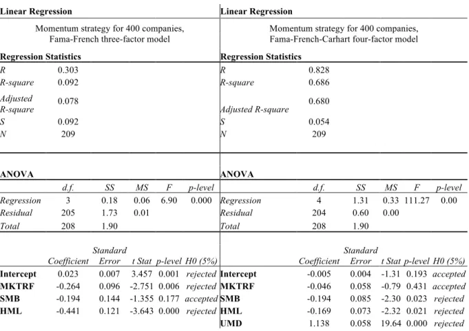
Table IV – Fama-French three-factor model (left) and Fama-French-Carhart four-factor model (right) for portfolio with 400 companies
Table V - Fama-French three-factor model (left) and Fama-French-Carhart four-factor model (right) for portfolio with 20 companies
Linear Regression Linear Regression
Momentum strategy for 20 companies, Fama-French three-factor model
Momentum strategy for 20 companies, Fama-French-Carhart four-factor model
Regression Statistics Regression Statistics
R 0.367 R 0.677
R-square 0.135 R-square 0.459
Adjusted
R-square 0.122
Adjusted
R-square 0.448 S 0.194 S 0.154
N 209 N 209
ANOVA ANOVA
d.f. SS MS F p-level d.f. SS MS F p-level Regression 3 1.20 0.40 10.62 0.000 Regression 4 4.10 1.03 43.26 0.000
Linear Regression Linear Regression
Momentum strategy for 400 companies, Fama-French three-factor model
Momentum strategy for 400 companies, Fama-French-Carhart four-factor model
Regression Statistics Regression Statistics
R 0.303 R 0.828
R-square 0.092 R-square 0.686
Adjusted
R-square 0.078 Adjusted R-square 0.680 S 0.092 S 0.054
N 209 N 209
ANOVA ANOVA
d.f. SS MS F p-level d.f. SS MS F p-level Regression 3 0.18 0.06 6.90 0.000 Regression 4 1.31 0.33 111.27 0.00
Residual 205 1.73 0.01 Residual 204 0.60 0.00
Total 208 1.90 Total 208 1.90
Coefficient
Standard
Error t Stat p-level H0 (5%) Coefficient
Standard
Error t Stat p-level H0 (5%)
Intercept 0.023 0.007 3.457 0.001 rejected Intercept -0.005 0.004 -1.31 0.193 accepted
MKTRF -0.264 0.096 -2.751 0.006 rejected MKTRF -0.046 0.058 -0.79 0.431 accepted
SMB -0.194 0.144 -1.355 0.177 accepted SMB -0.194 0.085 -2.30 0.023 rejected
HML -0.441 0.121 -3.643 0.000 rejected HML -0.169 0.073 -2.32 0.021 rejected
Residual 205 7.73 0.04 Residual 204 4.83 0.02
Total 208 8.93 Total 208 8.93
Coefficient
Standard
Error t Stat p-level H0 (5%) Coefficient
Standard
Error t Stat p-level H0 (5%)
Intercept 0.094 0.014 6.62 0.00 rejected Intercept 0.048 0.012 4.01 0.00 rejected
MKTRF -0.018 0.203 -0.08 0.93 accepted MKTRF 0.333 0.164 2.02 0.04 rejected
SMB -1.148 0.304 -3.78 0.00 rejected SMB -1.148 0.241 -4.77 0.00 rejected
HML -1.136 0.256 -4.435 0.00 rejected HML -0.700 0.207 -3.38 0.00 rejected
UMD 1.822 0.165 11.05 0.00 rejected
iii. Combination of both strategies
The last analysis that I’ve done in the search for a better performing variation of the
Momentum strategy was to combine the Base Strategy with a Value Strategy with the same
parameters and number of companies. Figure VI shows the stand-alone Sharpe Ratio of each
strategy, and the equivalent for the combined portfolio. For almost any number of companies,
the Sharpe Ratio is much higher when combining the two strategies than when investing in
just one, and also that the Momentum’s Sharpe Ratio only exceeds that of the combination
due to a sizable underperformance for the Value strategies for highly concentrated portfolios.
Figure VI - Sharpe Ratio for stand-alone strategies and combined strategy
-0.2 -0.1 0.0 0.1 0.2 0.3 0.4 0.5 0.6 0.7 0.8 0.9 1.0 1.1 5
20 35 50 65 80 95 110 125 140 155 170 185 200 215 230 245 260 275 290 305 320 335 350 365 380 395
S h ar p e R ati o
Number of Companies
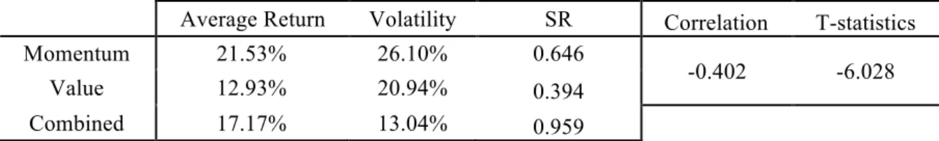
When analyzing the case of 100 companies in particular, it’s clear that the reason
behind this increase in Sharpe Ratio is the significant negative correlation between the two
strategies, which can be seen in Table VI and Figure VII. This negative correlation was also
found in Asness et al (2013).
Table VI - Return, volatility and Sharpe Ratio for each stand-alone strategy and for the combined strategy. Correlation between Momentum and Value strategies and its significance.
Average Return Volatility SR Correlation T-statistics Momentum 21.53% 26.10% 0.646
-0.402 -6.028 Value 12.93% 20.94% 0.394
Combined 17.17% 13.04% 0.959
For the variations analyzed, the optimal concentration for a Momentum-only portfolio
seems to be around 30 companies long plus 30 companies short, which led to an overall
Sharpe Ratio of around 0.8. This number of companies is substantially lower than that of the
optimal combined portfolio of Value and Momentum, which is around 90 companies for each
leg. This happens because the Value strategy has an optimal concentration of 230 companies
at a Sharpe Ratio of around 0.47, after which it stagnates. The estimated optimal Momentum
concentration differs from most studies done on the Momentum strategy, since the average
concentration observed in other studies is a decile of the three stock exchanges used here, for
example in Jegadeesh and Titman (2001), which nowadays results in around 500 companies,
Figure VII - Returns for stand-alone strategies and for the combined strategy
Note: Returns above are quarterly
VI. Limitations
Although most of the results obtained were in line with what was expected, there were
some limitations, which were made less severe due to the high number of companies in the
sample. An example of this is the amount of missing data from the database: although the
database is one of the largest, and has an immeasurable amount of information, there were
still many cases of firms that had missing returns, or cases where the return was available, but
the Market Cap wasn’t. The biggest challenge in terms of data was for the price-to-book
variable, which out of the 30,000 companies in the stock exchanges considered only 20,000
had values, and only starting in 1970. This limitation had a negative impact in another
situation: when creating the Value strategy to combine it with the Momentum, I tried to
impose the Market Cap lower limit of 100 million as done before, however since in this case
the number of data available was much smaller, this resulted in a too controlled strategy, and
for example if I wanted to long and short 400 companies, I could have only 500 that fit the
market cap criteria, and so I had to lower the lower the Market Cap limit to 1 million only, so
-80.00% -60.00% -40.00% -20.00% 0.00% 20.00% 40.00% 60.00% 80.00%
1965 1969 1973 1980 1984 1990 1997 2001 2005 2012 2016
R
etu
rn
s
Year
Momentum Value Combined
Number of Companies: 100 Ranking Period: 11
Lag: 1
that the ranking of price-to-books would have enough companies with the data necessary, for
all points in time. This is shown in Figure VIII, in the dotted line there are not enough
companies in the sample for the strategy to be done effectively, and so the Sharpe Ratio is
very low for any number of companies, and in the solid line there are enough companies in
the sample, and the strategy has a high Sharpe Ratio. This shows that withdrawing the
condition in this case has more pros than cons: it could have happened that the increase in
volatility that originates from including too many penny-stocks wouldn’t have compensated
the increase in return, but as a matter of fact, in this case the difference is almost completely
driven by an increase in return. Figures VIII.B and VIII.C in the Annexes file display their
average returns and standard deviations, and the Sharpe Ratio of the combined strategy if both
had been limited to a Market Cap superior to 100 million USD, respectively.
Figure VIII - Sharpe Ratio for Value strategy when limited to a Market Cap higher than 1 million and 100 million
An important consideration to have when studying any investment strategy are the
transaction costs. This paper didn’t take into consideration the eventual impact of transaction
costs in the strategy return. However, considering the results of Frazzini et al (2015) and the
-0.2000 -0.1000 0.0000 0.1000 0.2000 0.3000 0.4000 0.5000 0.6000
5
20 35 50 65 80 95 110 125 140 155 170 185 200 215 230 245 260 275 290 305 320 335 350 365 380 395
S
h
ar
p
e R
ati
o
Number of Companies
fact that the abnormal returns found in this paper are so significant, I do not consider that a
relevant limitation.
“We conclude that the main capital market anomalies – size, value, and momentum – are
robust, implementable, and sizeable in the face of transactions costs.“ (Frazzini et al, 2015: Page 1)
VII. Conclusion
Overall, the Standard Momentum strategy during the period between 1965 and 2015
has a 1.4% monthly statistically significant abnormal return as given by the Jensen’s Alpha
from the CAPM model, a result similar to the one found in Jegadeesh and Titman (2001) of
1.24% significant abnormal monthly return between 1965 and 1998. The sub periods of 1965
to 1989 and 1990 to 1998 also have significant abnormal returns for the variation of the
strategy studied in this paper, however the final period of 1999 to 2015 does not give a
significant overall abnormal return. Yet, by separating this, the period between 2012 and 2015
does yield a significant abnormal return of 2.9% monthly, while the period between 1999 and
2011 doesn’t because of the high volatility in the markets due to the financial crisis of 2002
and 2008. The Alpha Momentum strategy has a higher Sharpe Ratio than the Standard for the
overall period, with the exception of highly concentrated portfolios
When combining the Standard Momentum with a Value strategy, there is a negative
correlation between the two, and although the Value part of the portfolio reduces returns, the
decrease in volatility compensates and there is a large increase in Sharpe Ratio when
comparing with any of the two strategies alone.
VIII. Bibliography
Asness, Clifford S., Tobias J. Moskowitz and Lasse H. Pedersen. 2013. “Value and Momentum Everywhere.” The Journal of Finance, Vol. 68, No. 3, Pages 929–985
Barroso, Pedro and Pedro Santa-Clara. 2015. “Managing Momentum risks: Momentum has its Moments “ Journal of Financial Economics, Vol. 116, Issue 1, Pages 111-120
Black, Fischer. 1972. “Capital Market Equilibrium With Restricted Borrowing.” The Journal of Business, Vol. 45, No. 3, Pages 444-455
Blitz, David, Joop Huij and Martin Martens. 2011. “Residual Momentum.” Journal of Empirical Finance, Vol. 18, No. 3, Pages 506–521
Carhart, Mark M. 1997. “On Persistence in Mutual Fund Performance.” The Journal of Finance, Vol. 52, No. 1, Pages 57-82
Daniel, Kent and Tobias J. Moskowitz. 2015. “Momentum Crashes.” Journal of Financial Economics, Vol. 122, No. 2, Pages 221–247
De Groot, Wilma, Joop Huij and Weili Zhou. 2011. “Another Look at Trading Costs and Short-Term Reversal Profits.”Journal of Banking & Finance, Vol. 36, No. 2, Pages 371–382
Fama, Eugene F. 1969. “Efficient Capital Markets: A Review of Theory and Empirical Work.” The Journal of Finance, Volume 25, Issue 2, Pages 383-417
Fama, Eugene F. and Kenneth R. French. 1992. "The Cross-Section of Expected Stock Returns." The Journal of Finance, Vol. 47, No. 2, Pages 427–465
Fama, Eugene F. and Kenneth R. French. 2015. “A Five-Factor Asset-Pricing Model.” Journal of Financial Economics, Vol. 116, No. 1, Pages 1–22
Fisher, Gregg, Ronnie Shah and Sheridan Titman. 2016. “Combining Value and Momentum.” Journal Of Investment Management, Vol. 14, No. 2, Pages 33–48
Grundy, Bruce D. and J. Spencer Martin. 1998. “Understanding the Nature of the Risks and the Source of the Rewards to Momentum Investing.” The Review of Financial Studies,
Volume 14, issue 1, pages 29-78
Hühn, Hannah Lea and Hendrik Scholz. 2013. “Alpha Momentum and Price Momentum.”
Available at SSRN: https://ssrn.com/abstract=2287848
Jegadeesh, Narasimhan and Sheridan Titman. 1993. “Returns to Buying Winners and Selling Losers: Implications for Stock Market Efficiency.” The Journal of Finance, Vol. 48,
No. 1, pp. 65-91
Jegadeesh, Narasimhan and Sheridan Titman. 2001. “Profitability of Momentum Strategies: An Evaluation of Alternative Explanations.” The Journal of Finance, Vol. 56, No.
2, pp. 699-720
Lintner, John. 1965. “The Valuation of Risk Assets and the Selection of Risky Investments in Stock Portfolios and Capital Budgets.” The Review of Economics and Statistics, Vol. 47,
No. 1, Pages 13-37
Liu, Qianqiu, S. Ghon Rhee and Liang Zhang. 2011. “On the Trading Profitability of Penny Stocks.” 24th Australasian Finance and Banking Conference 2011 Paper. Available at
SSRN: https://ssrn.com/abstract=1917300
Sharpe, William F. 1964. “Capital Asset Prices: A Theory of Market Equilibrium under Conditions of Risk.” The Journal of Finance, Vol. 19, No. 3, Pages 425-442
Sharpe, William F. 1966. “Mutual Fund Performance.” The Journal of Business, Vol.39, No. 1, Part 2: Supplement on Security Prices. Pages 119-138
Wang, Kevin Q. and Jianguo Xu. 2015. “Market Volatility and Momentum.” Journal of Empirical Finance, Vol. 30, Pages 79–91