doi: 10.1590/0101-7438.2015.035.03.0509
A NEW MATHEMATICAL MODEL
FOR THE CUTTING STOCK/LEFTOVER PROBLEM
Marcos Nereu Arenales
1, Adriana Cristina Cherri
2*,
Douglas N. do Nascimento
3and Andr´ea Vianna
3Received October 2, 2014 / Accepted July 8, 2015
ABSTRACT.This paper addresses the cutting stock/leftover problem (CSLP), which differs from the or-dinary cutting stock problem (CSP) by retaining stock leftovers that can be cut in the future to meet new demands. Therefore, leftovers are not considered waste in the current period. A new mathematical model for the CSLP is presented to capture a well-used strategy in the practice of cutting, which consists of partially cutting the objects in stock, and keeping the leftovers to be cut in the next periods. Computa-tional experiments were made for the one-dimensional case, although other dimensions can be considered straightforward.
Keywords: cutting stock problem, usable leftovers, mathematical model, column generation.
1 INTRODUCTION
Cutting Stock Problems (CSP) are central stages in production planning for a number of indus-tries that have to cut paper rolls, steel bobbins, steel bars, wooden hardboards, leather pieces, among others. Basically, CSP consists of cutting large pieces (objects) available in stock into a set of smaller pieces (items) with specified quantities and sizes by optimizing an objective func-tion, such as minimizing the total length/area/volume of the objects cut, minimizing the total waste or minimizing the cost of the objects cut.
Although there are many articles in the literature on general CSP, many constraints arise in practical situations that lead to the need of developing new mathematical models and new ap-proaches to solve them. Among the various types of CSP in the literature (see W¨ascher et al. (2007), for a typology), a problem which has not been fully studied yet, although it often appears in practice, consists of considering usable leftovers when the objects are cut. These leftovers are
*Corresponding author.
1Instituto de Ciˆencias Matem´aticas e Computac¸˜ao, Universidade de S˜ao Paulo. E-mail: [email protected] 2Departamento de Matem´atica, Universidade Estadual Paulista J´ulio de Mesquita Filho. E-mail: [email protected] 3Departamento de Computac¸˜ao, Universidade Estadual Paulista J´ulio de Mesquita Filho.
kept in stock to meet future demands, and therefore they are not wasted. We call this problem the Cutting Stock/Leftover Problem (CSLP) and we may refer to it as 1D-CSLP if only one dimension is relevant in the cutting process, such as cutting bars and rolls.
A considerable amount of literature has been published on 1D-CSLP, see Cherri et al. (2014) for a survey. To the best of our knowledge, it was first mentioned by Brown (1971), but only to dif-ferentiate preferable solutions among others with some waste. Scheithauer (1991) proposed the first mathematical model for CSLP, which is a cutting pattern-oriented model (see Kantorovich, 1960; Gilmore & Gomory, 1961). The main idea in the Scheithauer model consists of consider-ing fictitious items (or residual lengths with no demand associated) that can be cut in the future. These fictitious items play the role of leftovers with special utility values. This approach reduces the waste by diversifying items (it is well-known that instances with a diversity of sizes of items have less waste). We call this as anitem-oriented approach. Cui & Yang (2010) extended the Scheithauer model to include upper bounds on the number of leftovers.
Anassignment approachis given by Abuabara & Morabito (2009), in which assigning or not an item to an object is a decision to be made. This approach is able to find optimal solutions for smaller instances. However, most of the methods in the literature are greedy heuristics that per-turb a good solution of the CSP in order to try to join waste together (Roodman (1986), Gradisar et al. (1997), Gradisar et al. (1999), Cherri et al. (2009, 2013), among others). In addition, they define bounds to determine the minimum acceptable length for the generated leftovers during the cutting process (see Cherri et al. (2014) for a survey). Thus, a great diversity of lengths of leftovers can be generated, which may be unacceptable to many industries since this needs ef-ficient control systems to retrieve them in the future, and a high risk of being wasted as well. This is not a conjecture, the authors have already witnessed this situation. In our approach to this paper, the same leftover types may always be found in stock, as the manager decides the sizes and quantities of the leftovers.
Andrade et al. (2013) and Andrade et al. (2014) presented multilevel MIP models to solve the two-dimensional cutting stock problem with usable leftovers. They used bounds to define leftover dimensions not allowing a control on the number of leftover types.
Cherri et al. (2014) reviewed papers from the literature that consider the1D-CSLP. In this survey, the authors present applications of the problems, the mathematical model (if it was proposed), comments on the results obtained from each paper and proposals for future studies related to the 1D-CSPUL.
The remainder of the paper is outlined as follows. In Section 2, the CSLP is defined and a mathe-matical model to solve it is proposed. The concepts concerning our strategy to solve the problem are also well quantified in this section. In Section 3, a solution method is described together with a small example to illustrate the solutions obtained by the proposed model. Computational results are given in Section 4. In Section 5, we present some concluding remarks.
2 THE CSLP OBJECT-ORIENTED MODEL
In the CSLP, a set of items must be produced by cutting large objects of standard sizes (objects bought on the market) or nonstandard (objects that are leftovers of previous cuts). Similarly to the CSP, there are given demands and sizes of items on one hand, and availabilities and sizes of objects, on the other. Demands must be met by cutting the available objects in stock in order to minimize waste, or another suitable objective function. However, new leftovers of given sizes can be generated within a limited amount, which are not counted as waste.
In summary, we consider the following practical assumptions:
1. Anystandard objectcan be completely cut or partially cut to generate two new objects: a reduced objectto be currently cut and aleftoverto be kept in stock for future demands;
2. Any leftover has its size given beforehand;
3. The total number of new leftovers is limited.
Data:
S: number of types of standard objects. We denote object types,s∈ {1, . . . ,S};
R: number of types of leftovers in stock. We denote leftover typeS+s,s∈ {1, . . . ,R};
es: number of objects/leftover typesavailable in stock,s=1, . . . ,S+R;
Ls: length of object/leftover types,s=1, . . . ,S+R;
m: number of types of ordered items;
di: demand for item typei,i=1, . . . ,m;
ℓi: length of item typei,i =1, . . . ,m;
Js: set of cutting patterns for object types,s=1, . . . ,S+R;
Js(k): set of cutting patterns for standard object typeswith leftover typeS+k,k=1, . . . ,R, s=1, . . . ,S;
ai j s: number of items type i in cutting pattern j for object type s, i = 1, . . . ,m,
s=1, . . . ,S+R, j ∈ Js;
ai j sk: number of items typei in cutting pattern j for object typesand leftover typeS+k,
cj s: waste of cutting object/leftoversaccording to pattern j,s=1, . . . ,S+R, j ∈ Js;
cj sk: waste of cutting objectsaccording to pattern j when generating a leftover typeS+k, s=1, . . . ,S,k=1, . . . ,R, j∈ Js(k);
U: maximum number of leftovers;
Variables:
xj s: number of objects typescut according to pattern j,s=1, . . . ,S+R, j∈ Js;
xj sk: number of objects types cut according to pattern j generating a leftover typeS+k, s=1, . . . ,S,k=1, . . . ,R, j∈ Js(k).
Remarks
1. The size of a reduced object obtained by partially cutting an object typeswith leftover typeS+kis given by:Ls−LS+k. Only standard objects can be cut with a leftover.
2. Although in Assumption 1 any standard object can be used to generate a leftover, it is possible to allow leftovers of only one type of object.
3. Assumptions 2 and 3 are considered to make operational handling feasible. Leftovers may be limited to only one size.
The CSLP Object-Oriented Model
Minimize f(x)=
S
s=1
j∈Js
cj sxj s+α′ S
s=1
R
k=1
j∈Js(k)
cj skxj sk
+α′′
S+R
s=S+1
j∈Js
cj sxj s (1)
subject to S
s=1
j∈Js
ai j sxj s+ S
s=1
R
k=1
j∈Js(k)
ai j skxj sk
+
S+R
s=S+1
j∈Js
ai j sxj s=di, i =1, . . . ,m (2)
j∈Js
xj s+ R
k=1
j∈Js(k)
xj sk ≤es, s=1, . . . ,S (3)
j∈Js
S
s=1
R
k=1
j∈Js(k)
xj sk−
S+R
s=S+1
j∈Js
xj s ≤U−
S+R
s=S+1
es (5)
xj s≥0, s=1, . . . ,S+R, j∈ Js;
xj sk ≥0, k=1, . . . ,R,
s=1, . . . ,S, j ∈ Js(k)and integer. (6)
Factorsα′≥1 andα′′≤1 in objective function (1) can be used to say that a new leftover should be created only if it is really attractive, or an older leftover should be cut although it produces more waste than other objects cut.
The objective function (1) to be minimized determines the total waste of cutting standard, with or without leftovers, and nonstandard (previous leftovers) objects. Constraints (2), (3) and (4) are demand and stock constraints, respectively. Constraint (5) limits the net quantity of leftovers, that is, no more thanU units of leftovers are allowed for the next period. Non-negativity and integrality of variablesxj sandxj sk are ensured by the constraint (6).
Because of the exponential number of variables and the integrality conditions, it is hard to solve model(1)-(6) at optimality. The linear relaxation, obtained by relaxing the integer condition in (6), can be easily solved with the column generation technique (Gilmore & Gomory, 1963) and good integer solutions can be found using heuristic procedures (see W¨ascher & Gau, 1996; Poldi & Arenales, 2009, among others). The linear relaxation enables us to analyze tendencies of gains, i.e., how much waste is expected to be diminished by using different policies on leftover stock and how these gains depend on data.
3 SOLVING THE LINEAR RELAXATION OF THE CSLP OBJECT-ORIENTED
MODEL
Before describing the column generation technique (Gilmore & Gomory, 1963; Desaulniers et al., 2005) for the CSLP object-oriented model, we show how to price each column. Suppose model (1)-(6) has been solved using a few columns, called theRestricted Master Problem, and the simplex multiplier (dual variable) is given by(π1π2π3π4), whereπ1is am-vector,π2a S-vector,π3aR-vector, andπ4a real number, associated to constraints (2)-(5) respectively.
We distinguish three cases:
a) Standard objects,s∈ Js,s=1, . . . ,S
A general column associated toJs is given by (index jis omitted):
as =
a1s · · ·ams
m-vector
pattern
| 0· · ·1· · ·0
S-vector
identity column
| 0· · ·0
R-vector
of zeros
where the firstm-vector corresponds to a cutting pattern for a standard object size Ls. Sinceℓi is the length of itemi,i=1, . . . ,m, the reduced cost associated to this column is:
ˆ
c(as) = Ls− m
i=1 ℓiais
cs: waste
−
m
i=1
πi1ais−πs2
= −
m
i=1
ℓi+πi1
vi
ais +(Ls−πs2)
b) Reduced objects (or standard objects with leftover),s∈ Js(k),k=1, . . . ,R,s=1, . . . ,S
Suppose a cut generates a leftover, then a general column associated toJs(k)is given by (index jis omitted):
as(k)=
a1s · · ·ams
m-vector
pattern
| 0· · ·1· · ·0
S-vector
identity column
| 0· · ·0
R-vector
of zeros
|1T
where the first m-vector corresponds to a cutting pattern for the reduced object Ls −LS+k. Therefore, the reduced cost associated to this column is:
ˆ
c(as(k)) = α′ (Ls −LS+k)− m
i=1 ℓiais
cs: weighted waste
−
m
i=1
πi1ais−πs2−π4
= −
m
i=1
(α′ℓi +πi1
vi
)ais+(α′(Ls −LS+k)−πs2−π4)
c) Leftover objects,s∈ Js,s=S+1, . . . ,S+R
A general column associated toJs,s=S+1, . . . ,S+Ris given by (index jis omitted):
as=(a1s · · ·ams
m-vector
pattern
| 0· · ·0
S-vector
of zeros
| 0· · ·1· · ·0
R-vector
identity column
| −1)T
where the firstm-vector corresponds to a cutting pattern for a leftoverLs. Therefore, the reduced cost associated to this column is:
ˆ
c(as) = α′′ Ls− m
i=1 ℓiais
cs: weighted waste
−
m
i=1
= −
m
i=1
(α′′ℓi+πi1
vi
)ais+(α′′Ls−πs3+π4)
In summary, we have three cases:
a) For a standard object types:
ˆ
c(as)= − m
i=1
viais +(Ls−πs2),
wherevi =ℓi +πi1, and(a1s. . .ams)Tcorresponds to a cutting pattern for lengthLs;
b) For a reduced object obtained from a standard objects:
ˆ
c(as(k))= − m
i=1
viais+((α′Ls−LS+k)−πs2−π4)
wherevi =α′ℓi +πi1and(a1s. . .ams)Tcorresponds to a cutting pattern forLs−LS+k;
c) For a leftover in stock types:
ˆ
c(as)= − m
i=1
viais+(α′′Ls−πs3+π
4)
wherevi =α′′ℓi+πi1, and(a1s. . .ams)Tcorresponds to a cutting pattern toLs.
The column generation technique is summarized as follows:
Initial step: Build a restricted master problem, i.e., model (1)-(6) with few columns that use trivial cutting patterns, such as homogeneous cutting patterns for standard objects and leftovers. If necessary, include artificial variables. Iteration:t =0.
Step 1.Solve the linear relaxation of the restricted master problem in iterationt.
Step 2.
2.1 –Fors=1, . . . ,S
Solve the cutting problem (vi is the utility value given in case a))
Maximizev1a1s+ · · · +vmams
subject to:(a1s· · ·ams)is a cutting pattern toLs
calculate the correspondent column and the reduced cost according to case a);
2.2 –Fors=1, . . . ,S
Maximizev1a1+ · · · +vmam
subject to: (a1s· · ·ams) is a cutting pattern toLs−LS+k,k=1, . . . ,R calculate the correspondent column and the reduced cost according to case b);
2.3 –Fors=S+1, . . . ,S+R
Solve the cutting problem (vi is given in case c))
Maximizev1a1+ · · · +vmam
subject to that (a1s. . .ams) is a cutting pattern toLs
calculate the correspondent column and the reduced cost according to case c).
Step 3. Include the most attractive column (i.e., column withthe most negative reduced cost found in steps 2.1, 2.2 or 2.3) to the restricted master problem. If no attractive column is found, stop – the current solution obtained in Step 1 is an optimal solution to the linear relaxation of model (1)-(6); otherwise, dot =t+1 and go to Step 1.
Example
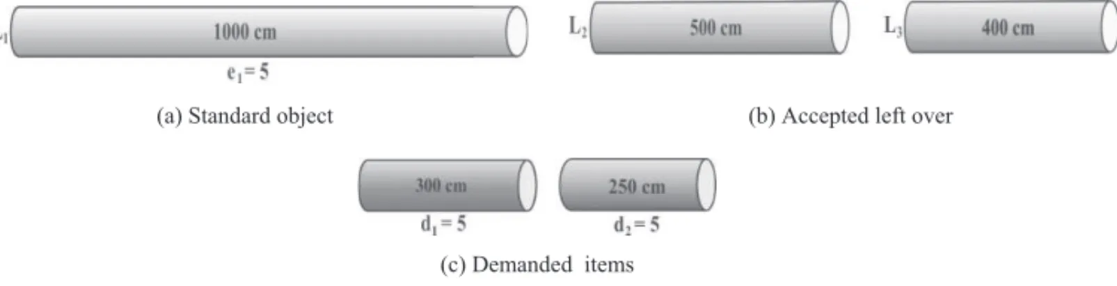
In order to make the presentation clear, we solved problem (1)-(6) for a very small instance, for which all columns can be easily generated beforehand and the integrality conditions can be taken into account using an optimization package. In addition, we also give the continuous solution obtained by the column generation technique described previously. Figure 1 shows the data for a CSLP.
(a) Standard object (b) Accepted left over
(c) Demanded items
Figure 1– (a)-(c) Data of a cutting stock/leftover problem.
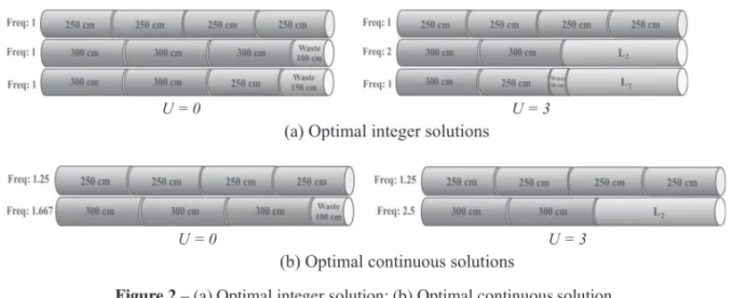
that can better allocate the new demands. For the present period the waste is reduced from 250 to 50 (Fig. 2(a)), and there is a great opportunity to reduce the waste in the next period because the more the object sizes there are to be cut, the less waste there is. This simple instance also shows that the manager has the possibility of dealing with other sizes, if it is acceptable. For example, the leftover in the third cutting pattern forU = 3 in Figure 2(a) can be seen as it sized 450, instead of 400 plus a waste of 50.
U = 0 U = 3
(a) Optimal integer solutions
U = 0 U = 3
(b) Optimal continuous solutions
Figure 2– (a) Optimal integer solution; (b) Optimal continuous solution.
4 COMPUTATIONAL EXPERIMENTS
To evaluate the performance of the proposed approach in order to analyze waste reduction, 6 classes of instances were considered, by varying lengths and demand of items. For each class, 50 instances were randomly generated. The tests were divided considering two situations. Firstly, we simulated the initial period of the cutting process where there were no leftovers in stock, but considering or not the possibility of generating leftovers. Note that by avoiding the generation of new leftovers together with no leftover in stock, the problem coincides with the classical cutting stock problem. The second situation simulated an intermediate period with leftovers already available in stock.
For both situations, initial or intermediate periods, the stock only had one type of standard ob-ject with length L1 = 1000 and availability large enough to meet the demands. Three types
of leftovers were considered with lengths 400, 500 and 600. The availabilities of leftover type s = 1,2, and 3 werees = 0, for the initial period, andes = k, k = 0 to 3, for the interme-diate period. The maximum quantity of leftovers varied asU = 3k+3,k = 0 to 3. We also consideredα′=α′′=1 in the objective function (1), that is, the overall waste to be minimized, not intending to encourage the generation of new leftovers nor to be obliged to use the leftovers in stock.
Each instance hadm = 15 types of demanded items. Lengthℓi of item typei was randomly generated in the interval[v1L1, v2L1]. We call itmedium item(M)ifv1=0.14 andv2=0.4 (a
2 to 3 items). Small demands(S)are generated in the interval[1,10],medium demands(M)in the interval[10,50]andbig demand(B)in[50,300]. Therefore, a class [B,S] means a set of 50 instances where items are big, and demands are small. The exact values of all the instances we have used can be obtained by contacting the corresponding author.
The proposed method was coded using OPL (Optimization Programming Language) of the soft-ware CPLEX, version 12.5. The computational tests were run on a computer Core i7, 3.07 GHz x8, 8 GB RAM. The average computation time for each instance was approximately 56 seconds.
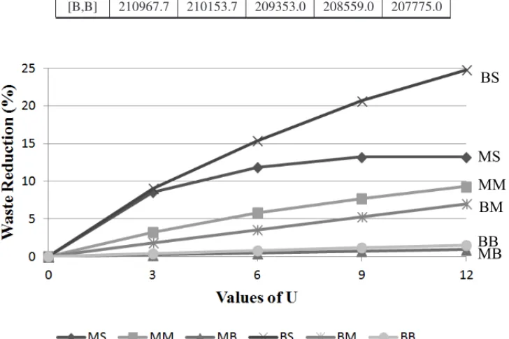
Table 1 shows the results for the first period where it is supposed that no leftover is in stock. Note that columnU =0 consists of the classical cutting stock problem, with no leftovers in stock and no leftover is allowed to be generated. The average waste is given in terms of different values of U. Note that we adopted the total waste to define the objective function, but the total length used could be considered instead. Both are well-used in practice. Graph 1 shows the percentage waste evolution in terms ofUrelated to the classical CSP in the first column in Table 1.
Table 1– Waste for the first period: no leftovers in stock.
Class U=0 U=3 U=6 U=9 U=12
[M,S] 136.9 125.1 120.7 118.8 118.8
[M,M] 634.1 613.9 597.5 585.6 575.2
[M,B] 3599.2 3590.3 3581.6 3573.1 3564.7
[B,S] 6971.7 6343.0 5899.7 5530.9 5243.5
[B,M] 39541.7 38830.4 38137.0 37455.0 36787.0
[B,B] 210967.7 210153.7 209353.0 208559.0 207775.0
MM
BM BS
BB MB MS
These results point out some features. It does not matter if the leftover strategy is used or not when demands are big. This was already expected because the bigger the demands, the more possibilities there are of arranging items in the object so that there is nothing or little to be reduced by generating new leftovers. Of course, the bigger the item sizes, the higher the waste.
Interesting cases happen when the demands are small – classes [M,S] and [B,S], typical cases of small industries, where the wasteis 136.9 and 6971.7, respectively, for the strategy of no leftovers – the classical cutting stock problem. However, by usingU= 12, the waste is respectively 118.8 and 5243.5, which means reductions of 13.2% and 24.8%. Considering that in small industries, raw materials have the most important part of the overall cost of final products, this reduction can make them competitive in the market. Despite the fact that waste decreases as demands increase, irregularity of demands is also common for small industries, so that keeping items in stock – the item oriented approach – may be unacceptable. It is also worth noting that small demands for the cutting problem can occur for larger industries, such as the agricultural light aircraft industry in Abuabara & Morabito (2009). In summary, the situations of small to medium demands together with big to medium items are the most promising situations to allow for leftovers during the cutting process.
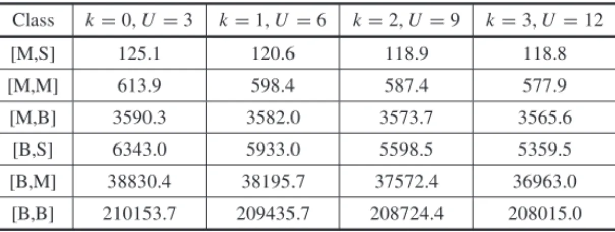
The following experiments consider an intermediate period, where alongside the standardized objects are also leftovers from previous periods. We started with no leftovers in stock and in-creased them one by one. Furthermore, the value of the upper boundUvaried together with the availability of leftovers to make the stock consistent, but not too tight so that the generation of new leftovers is avoided. That is, fork =0 to 3,es = k,s =1,2,3, andU =3k+3. Note that ifk = 0, thenes =0,s =1,2, and 3, which means that there is no leftover in stock, but there is a possibility of generatingU =3 new leftovers. This is a real possibility, which is not only for the initial period. Table 2 shows the average waste in 50 instances, and Graph 2 depicts the percentage waste evolution in terms ofU related to the classical CSP (k=0,U =0). The results are quite similar to the first period.
Table 2– Waste for an intermediate period: leftovers in stock.
Class k=0,U=3 k=1,U=6 k=2,U=9 k=3,U=12
[M,S] 125.1 120.6 118.9 118.8
[M,M] 613.9 598.4 587.4 577.9
[M,B] 3590.3 3582.0 3573.7 3565.6
[B,S] 6343.0 5933.0 5598.5 5359.5
[B,M] 38830.4 38195.7 37572.4 36963.0
[B,B] 210153.7 209435.7 208724.4 208015.0
BM MS
MM
BB MB BS
Graph 2– Percentage waste for an intermediate period related tok=0,U=0.
The result gave a waste of 5124, and the leftovers sized 400 and 500 were fully used, and no leftover sized 600 was used. On the other hand, if the stock of leftovers were 6 units for size 400 and 3 units for size 500, summing 9 as before, the waste would be 4824, which means a waste reduction of 5.6%. This simple example shows that the model (1)-(6) can also be used for lot sizing the leftover stock. Similarly, different sizes of the leftovers can also be tested, that is, the manager can deal with the assortment problem.
5 CONCLUSIONS AND FINAL REMARKS
In this article, we presented a new mathematical model to describe the practical procedure of al-lowing partial cutting of objects in stock, creating leftovers to be cut in the future. First versions and discussions of this model were presented in the 9thESICUP (EURO Special Interest Group on Cutting and Packing) in La Laguna, Spain, 2012, and in the CMAC (Brazilian Congress of Applied Mathematics and Computing), Bauru, Brazil, 2013. This simple and practical mathemat-ical model represents the well-known fact that the diversity of object types in stock makes waste reduction possible. The idea of producing leftovers in order to reduce the waste is well-known in the literature, but only recently have researchers paid more attention to this problem.
Although we have fixed the leftover sizes, the manager might decide to add the waste in the cutting pattern to the leftover size. Of course, this makes increasing the number of different leftover types which demands a higher control system.
In addition, model (1)-(6) is quite general and flexible to deal with higher dimensions, as the dimension and additional constraints of the cutting process is embedded in the pattern generation in Step 2 of the Column Generation Algorithm (see Section 3). For example, in cutting plates sizedL×W, the manager can decide to have leftovers sizedLs×W, and/orL×Ws, by cutting the current demand using reduced objects sized(L−Ls)×W and/orL×(W−Ws). Therefore, in Step 2 of the Column Generation Algorithm, the objective function is subject to (a1s. . .ams) to be a cutting pattern for the plates(L−Ls)×W, orL ×(W −Ws). The way a plate is cut, such as guillotined, 2-staged etc., determines the constraints in the pricing problem.
In order to solve the integer CSLP, heuristics can be designed as extensions of the residual heuris-tic in Poldi & Arenales (2009). Residual heurisheuris-tics work as the following: solve LP relaxation of problem (1)-(6) and create rules to round the continuous solution to obtain integer values for the variables. Then, update demands and stocks, and repeat the steps. By solving the pricing problems with upper bounds on the number of items, so that any cutting pattern generated can be used at least once, the residual heuristics always converge.
ACKNOWLEDGMENTS
This research has been supported by theFundac¸˜ao de Amparo a Pesquisa do Estado de S˜ao Paulo (FAPESP) and theConselho Nacional de Desenvolvimento Cient´ıfico e Tecnol´ogico(CNPq). The authors are also indebted to the three anonymous referees.
REFERENCES
[1] ABUABARAA & MORABITOR. 2009. Cutting optimization of structural tubes to build agricultural light aircrafts.Annals of Operations Research,169: 149–165.
[2] ANDRADER, BIRGINEG, MORABITOR & RONCONIDP. 2013. MIP models for two-dimensional non-guillotine cutting problems with usable leftovers.Journal of the Operational Research Society, 65: 1649–1663.
[3] ANDRADER, BIRGINEG & MORABITOR. 2014. Two-stage two-dimensional guillotine cutting stock problems with usable leftovers.International Transactions in Operational Research, to appear (DOI: 10.1111/itor.12077).
[4] BROWN AR. 1971. Optimum packing and depletion: the computer in space and resource usage proble. New York: Macdonald – London and American Elsevier Inc, 107 p.
[5] CHERRIAC, ARENALESMN & YANASSEHH. 2009. The one-dimensional cutting stock problems with usable leftovers: A heuristic approach.European Journal of Operational Research,196: 897– 908.
[7] CHERRI AC, ARENALES MN, YANASSE HH, POLDI KC & VIANNA ACG. 2014. The one-dimensional cutting stock problem with usable leftovers – A survey.European Journal of Operational Research,236: 395–402.
[8] CUIY & YANGY. 2010. A heuristic for the one-dimensional cutting stock problem with usable leftovers.European Journal of Operational Research,204: 245–250.
[9] DESAULNIERSG, DESROSIERSJ & SOLOMONMM. (Eds). Column Generation. Springer Science and Business Media, Inc., 2005. 358 p.
[10] GILMOREPC & GOMORYRE. 1961. A linear programming approach to the cutting-stock problem.
Operations Research,9: 849–859.
[11] GILMOREPC & GOMORYRE. 1963. A linear programming approach to the cutting stock problem – Part II.Operations Research,11: 863–888.
[12] GRADISARM, JESENKOJ & RESINOVICC. 1997. Optimization of roll cutting in clothing industry.
Computers and Operational Research,10: 945–953.
[13] GRADISARM, KLJAJICM, RESINOVICC & JESENKOJ. 1999. A sequential heuristic procedure for one-dimensional cutting.European Journal of Operational Research,114: 557–568.
[14] KANTOROVICHLV. 1960. Mathematical methods of organizing and planning production. Manage-ment Science,6: 366–422.
[15] POLDIKC & ARENALESMN. 2009. Heuristics for the one-dimensional cutting stock problem with limited multiple stock lengths.Computers and Operations Research,36: 2074–2081.
[16] ROODMANGM. 1986. Near-optimal solutions to one-dimensional cutting stock problem.Computers and Operations Research,13: 713–719.
[17] SCHEITHAUERG. 1991. A note on handling residual length.Optimization,22: 461–466.
[18] W ¨ASCHERG & GAUT. 1996. Heuristics for the integer one-dimensional cutting stock problem: a computational study.OR Spektrum,18: 131–144.