The
Expansion and the Principle of Minimal Sensitivity
G.Kreina
, D.P. Menezes b
, M. Nielsen c
and M.B.Pinto b
a
Institut fur Kernphysik, Universitat Mainz, D-55099 Mainz, Germany
and
Instituto de Fsica Teorica, Universidade Estadual Paulista, Rua Pamplona 145, 01405-900 S~ao Paulo-SP, Brazil
b Departamento de Fsica, Universidade Federal de Santa Catarina
88.040-900 Florianopolis, S.C., Brazil
cInstituto de Fsica, Universidade de S~ao Paulo, Caixa Postal 66318
05315-970 S~ao Paulo, S.P., Brazil
Received December 5, 1997
The-expansion is a nonperturbative approach for eld theoretic models which combines
the techniques of perturbation theory and the variational principle. Dierent ways of imple-menting the principle of minimal sensitivity to the-expansion produce in general dierent
results for observables. For illustration we use the Nambu{Jona-Lasinio model for chiral symmetry restoration at nite density and compare results with those obtained with the Hartree-Fock approximation.
The standard application of the linear-expansion
[1] to a theory with actionS starts with an
interpola-tion dened byS() = (1,)S 0(
) +S, whereS 0(
)
is the action of a solvable theory. The actionS()
in-terpolates between the solvableS 0(
) (when= 0) and
the originalS (when = 1). Since S
0 is quadratic in
the elds, arbitrary parameters () with mass
dimen-sions are required for dimensional balance. At the end one sets = 1 xing according to the principle of
minimal sensitivity (PMS) [2] which requires a physical quantity () to satisfy
@() @
= 0: (1)
Within this method, the general procedure is to ap-ply the PMS directly to each dierent quantity of inter-est so as to adjustto the dierent energy scales of the
theory [2]. A natural question which arises at this point is the uniqueness of the value ofsince dierent
phys-ical quantities might generate dierent values for the optimal. Of course this would not be catastrophic if
the spread of the values ofdetermined from dierent
observables were not too large.
Alternatively, one could select only one among those
observables to optimize the theory. This selection could be done by using some physical criterion or constraint (for example, in the case were only one of the calcu-lated quantities satises the PMS equation). However, this strategy (referred as PMS1) does not completely specify a unique procedure and, as we shall see, can be misleading. One of our goals is to show that all these potential uncertanties could be avoided by demanding that fundamental quantities, such as the energy den-sity, be used to x whose optimal values are then
used to calculate other observables. Using the energy momentumtensor of the original theory one can obtain the exact energy density written in terms of full ver-tices and propagators. Next, one uses the interpolated theory to evaluate self energies as well as vertex correc-tions perturbatively in powers of. These-dependent
quantities are then plugged back into the energy density to which the PMS is applied. This approach (referred as PMS2) has been succesfully applied to the Walecka model for nuclear matter [3]. The fact that it is natu-ral to demand stationarity of the energy with respect to unknow parameters uniquely selects this quantity as
the generator of so that all physical observables are
determined from the same propagator.
In this paper we illustrate the problem with the PMS1 prescription by using the Nambu{Jona-Lasinio (NJL) model [4] for chiral symmetry restoration in a medium of nite density. Conventionally, the nite density chiral symmetry restoration problem within the NJL model has been tackled with the Hartree-Fock (HF) approximation. For the SU(2) case, this analyt-ical approach shows that chiral symmetry is restored through a rst-order phase transition at a critical den-sity whose values depend on the choice of the parame-ters [5, 6]. We then follow the two alternatives, PMS1 and PMS2, and compare results with the traditional HF approach.
Some physical quantities of interest, whose values characterize the chiral symmetry restoration, are the quark condensate
, the pion decay constantf and
the constituent quark mass M
q. We calculate these
quantities both with PMS1 and PMS2 and compare our
results with the ones obtained in Ref. [5] with the HF approximation, where vertex corrections are neglected. Therefore, we shall also neglect vertex corrections. Of course, since the NJL model is essentially phenomeno-logical, we shall pay more atention to the qualitative results (like the order of the phase transition) than to the quantitative ones (like the precise value of the crit-ical density for which the phase transition takes place). In the limit of zero current quark masses, the two-avor Lagrangian density of the Nambu{Jona-Lasinio model is given by
L
NJL=
q(i@/)q+G h
(q q) 2
,(q 5
q) 2
i
; (2)
where the quark eld operatorsq=q(x) represent the
doublet ofuanddquarks.
Let us start by deriving the energy density from the energy-momentum tensor of the original theory since this quantity will be necessary when using the PMS2. Using the Lagrangian density, Eq. (2), we have the energy-momentum tensor,
c
T
NJL= iq
@
q,g
L
NJL= iq
@
q,g
n
q(i@/)q+G h
(q q) 2
,(q 5
q) 2
io
: (3)
Note that we have not used the equation of motion for the quark eld operator. Neglecting vertex corrections, the energy density is given by
E
NJL = 1 V
Z
d 3
x <T 00
>
= ,i Z
d 4
q
(2) 4
q 0Tr
0
S(q)
+i Z
d 4
q
(2) 4Tr[
6q S(q)],G (
, Z
d 4
q
(2) 4Tr[
S(q)]
2
+Z d
4
q
(2) 4
d 4
k
(2) 4Tr[
S(q)S(k)] + Z
d 4
q
(2) 4Tr[
5 S(q)]
2
, Z
d 4
q
(2) 4
d 4
k
(2) 4Tr[
5
a
S(q) 5
a
S(k)]
; (4)
where S(q) represents the dressed quark propagator.
The quark condensate, which is taken to be the parameter of order of the phase transition, is given by
q q
=,i Z
d 4
p
(2) 4tr[
S(p)]; (5)
where the trace is taken over spinor and color indices. As in Refs. [5, 6] we employ the Pagels-Stokar formula [7] to evaluate the pion decay constant (f
), iq
f
ab= Z
d 4
p
(2) 4tr
S(p+q)(g q
5
a)
S(p)(12 b
5)
where the trace is now over spinor, avor and color. The quark-pion coupling can be obtained from the Golberger-Treiman relation. Of course, we could use other, perhaps more precise formulas for f
, but for our purposes of
comparing PMS1 and PMS2 results, Eq. (6) is sucient.
To dene the interpolated Lagrangian one needs to choose a solvable theory. Since we are looking for solutions which break chiral symmetry, the natural choice forL
0is L
0=
q(i@/,)q; (7)
whereis an arbitrary mass parameter. Therefore, the interpolated NJL Lagrangian density can be written as L
NJL(
) = (1,)
q(i@/,)q
+ n
q(i@/)q+G h
(q q) 2
,(q 5
q) 2
io
= q(i@/,)q+ n
G h
(q q) 2
,(q 5
q) 2
i
+q q o
: (8)
Expressed in terms of self energy (
p) the quark propagator reads S ,1(
p) = S ,1
0 ( p),
(
p) where S ,1
0 ( p)
is the inverse of the quark propagator corresponding to L 0 (
S ,1
0 (
p) =6p,), and the quark self-energy (
p) is
calculated as a power series in.
At zeroth order in , one is treating the free Lagrangian and hence (0)(
p) = 0. The bare (zeroth order)
in-medium quark propagator is then given by
S (0)(
p) =
6p+ p
2
, 2+
i
+ i 6p+ E
0( p)
,
p 0
,E
0( p)
(P F
,jpj) ; (9)
where E 0(
p) = ,
p 2+
2
1
2, and P
F is the Fermi momentum which, for N
f = 2, relates to the quark density via P
F = (
2
=2) 1=3.
At this order in, no dynamical content from the model has been used. The dynamics of the model starts to
show up at order. To O() the self-energy ( (1)(
p)) is given by
(1)(
p) = ,
+ 2iG Z
d 4
q
(2) 4
n
Trh S
(0)( q)
i
,S (0)(
q), 5
aTr
h
a
S (0)(
q) 5
i
+ 5
a
S (0)(
q) a
5 o
; (10)
where a sum over the isospin index a is implied. Substituting Eq. (9) into this equation, we obtain for (1) the
expression
(1)(
p) =,+M 1
,
00
; (11)
where
M
1 =
G
2
N
c N
f+ 12
8
<
:
,
2+
2
1
2
,P
F ,
P 2
F+
2
1
2
, 2ln
2
4 + ,
2+
2 1
2
P
F+ ( P
2
F+
2) 1
2 3
5 9
=
;
; (12)
and
0= ,4G
Z
d 3
q
(2) 3
(P F
,jqj): (13)
One should note that, at this order, direct and exchange terms are treated at equal footing as implied by the factor (N
c N
f + 1
=2) in Eq. (12). Since the eect of
0 is just to shift the chemical potential [6], one may write the
constituent quark mass toO() as
M
q =
,+M 1
: (14)
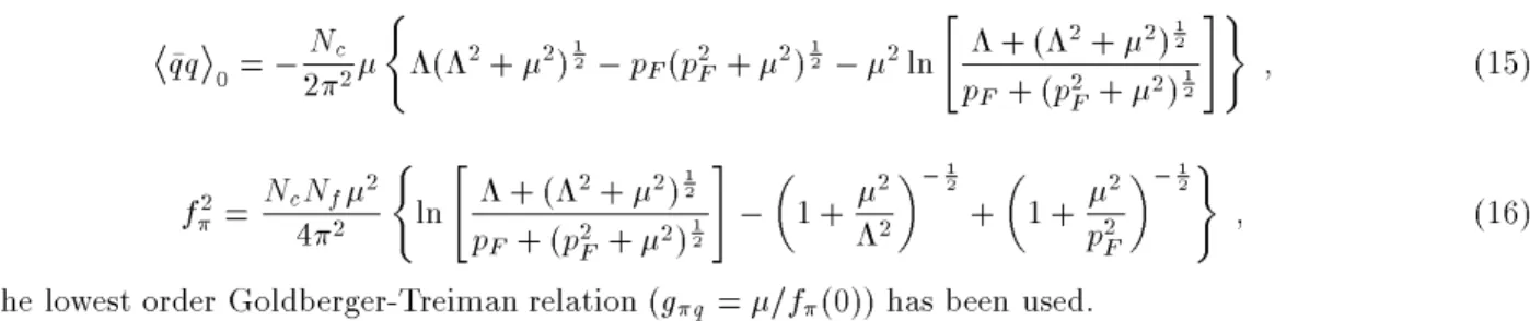
q q
0= ,
N
c
2 2
(
(2+
2) 1
2
,p
F( p
2
F+
2) 1
2
, 2ln
"
+ (2+
2) 1
2
p
F+ ( p
2
F+
2) 1
2 #)
; (15)
and
f 2
= N
c N
f
2
4 2
(
ln
"
+ (2+
2) 1
2
p
F+ ( p
2
F+
2) 1
2 #
,
1 + 2
2
, 1
2
+
1 + 2
p 2
F
, 1
2 )
; (16)
where the lowest order Goldberger-Treiman relation (g q =
=f
(0)) has been used. d
Figure1. PF dep endenceofobtained withthe PMS
ap-plied tof(solidline-PMS1)andto(dashedline-PMS2).
Figure2. PF dep endenceoff. Thesolid anddottedlines
giveresp ectivellythePMS1andthePMS2solutions.
We now have the three quantites of interest (M q,
q q
0and f
) obtained at lowest order in
and the next
step is the optimization procedure. Let us start with the PMS1. Of the three calculated quantities the only one which satises the PMS condition (the one which has extremum points) isf
. Moreover, at zero density,
this quantity has a well established empirical value and can be chosen to x. A direct application of the PMS
condition tof
gives
= 0:97. Using the zero
den-sity empirical valuef
= 93 MeV one gets the
non-covariant cut-o = 571 MeV. In principle, the fact that the cut-o can be xed (with a value which agrees with the ones used in the literature) without any pre-vious knowledge of the quark mass could be seen as an advantage of the method. However, one must be careful with the interpretation of this result since it has been obtained without any information about the model, be-cause the coupling constant Gdoes not appear at this
lowest order evaluation off
. If one takes this value for
and proceeds blindly by applying the PMS tof for
dierent values ofP
F one obtains
as a function of the
density as shown by the continuous line of Fig. 1. We note that obtained with the PMS1 has a very peculiar
behavior increasing with the density. This odd behav-ior is reected in Fig. 2 where one sees that f
goes
smoothly to zero, indicating chiral symmetry restora-tion, through a second-order phase transirestora-tion, contrary to the HF predictions. The same values of can be
used to evaluate the quark condensate and quark mass. The numerical zero density results for these quantities,
q q
0 =
,(250 MeV) 3 and
M
q = 574 MeV ( where
the valueG= 8:8610
,6 MeV ,2
was used in Eq. (12) forM
q) are not far from the ones predicted in the
lit-erature when a noncovariant cut-o is used. However, the nite density behavior of these two quantities again points out towards a smooth second-order phase tran-sition.
Let us now evaluate the same quantities using the PMS2 to generate the density dependent optimal values for . Substituting the lowest order quark propagator
c
E (0)
NJL= ,2N
c N f Z P F d 3 q
(2) 3 q 2 E 0( q)
,2GN c N f(2 N c N
f + 1) " Z P F d 3 q
(2) 3 E 0( q) # 2 : (17)
The requirement thatE be stationary with respect to variations inleads to
= 4G
N
c N
f+ 12 Z P F d 3 q
(2) 3 E 0( q) ; (18)
from where we immediately see that, even at zeroth order in , the value of depends on G, in contrast to the
result obtained with PMS1. Note that this is the familiar Hartree-Fock gap equation of the model, where has the
interpretation of the dynamically generated mass as can also be seen from its behavior at nite densities displayed in Fig. 1 (dashed line). As expected, when these optimal values are injected inf
, q q 0 and M
q, one predicts the
restoration of chiral symmetry through a rst-order phase transition in agreement with the HF results as can be seen by the dotted line in Fig. 2.
Next, one could try to improve these results by using the O() quark propagator in the evaluation of the energy
density. Inversion of Dyson's equation leads to
S (1)(
p) = 6p 1+ M 1 p 2 1 ,M 2 1+ i
+ i 6p 1+ M 1 E 1( p) , p 0 1 ,E 1( p) (P F
,jpj) ; (19)
where
p
1 = ( p
0
1
;p) = (p 0+
0
;p) ; E 1(
p) =
p 2+ (
M 1) 2 1 2 ; (20)
with 0 given by Eq. (13). The superscript (1) in S
(1) indicates that the propagator has been obtained with a
self-energy calculated up to rst-order in (note that the term , appearing in Eq. (14) has already been
discarded in Eq. (19)). Using the rst-order quark propagator in the evaluation of the energy density one gets
E (1)
NJL= ,2N
c N f Z PF d 3 q
(2) 3 q 2 E 1( q)
,2GN c N f(2 N c N
f + 1) " Z PF d 3 q
(2) 3 M 1 E 1( q) # 2 : (21)
An application of the PMS toE (1) NJL, dE (1) NJL d = dE (1) NJL dM 1 dM 1 d
= 0; (22)
leads to
M
1= 4 G
N
c N
f + 12 Z P F d 3 q
(2) 3 M 1 E 1( q) : (23)
Again, we have obtained the familiar Hartree-Fock gap equation for the dynamically generated mass.
d
Higher-order corrections will in general introduce a momentum dependence for the dynamically generated mass. However, if one proceeds to higher orders in
but neglect those graphs that correspond to vertex cor-rections, the higher-order quark propagator will always be of the form of Eq. (19), withM
1replaced by another
constant, sayM, which is a function of. However,
be-cause of the PMS condition onE,M at each order will
always be given by the same value. This value is the one that satises the usual gap equation
M = 4G
N
c N
f+ 12 Z P F d 3 q
(2) 3
M
E(q)
; (24)
where
E(q) = , q 2 +M 2 1 2 : (25)
(PMS2) is equivalent to the usual Hartree-Fock solu-tion for the dynamically generated mass, when vertex corrections are neglected.
To conclude, in this paper we have used the NJL model to illustrate potential problems with the applica-tion of the PMS in theexpansion. In order to specify
a unique prescription to x arbitrary parameters intro-duced by the expansion, we have studied two ways of
introducing the PMS procedure. We have applied the PMS directly to f
following the standard procedure
(PMS1) [2]. We found that PMS1 leads to results for chiral symmetry restoration that disagree with the HF results. Having a close look in the way the PMS1 trades
by the model parameters (the cut-o in this case) and
its nite density behavior, we were able to identify the origin of this misleading result. We have also applied the PMS to the energy density (PMS2). We have shown that this prescription reproduces, already at lowest or-der, the HF results for chiral symmetry restoration at nite density within the NJL model. Moreover, this re-sult can be reproduced at any order in provided that
one ignores vertex contributions. This result should be compared with the one presented in Ref. [8] where, in the context of the eective potential, it was found that theexpansion and the 1=N expansion are identical in
the large N limit. Therefore, the PMS2 seems to be
an adequate way of xing the arbitrary parameters to
generate nonperturbative results, and it is a promiss-ing procedure since it allows the introduction of vertex corrections in a very direct way. Work in this direction is in progress [9].
Acknowledgments
This work was partially supported by the Alexander von Hulboldt Foundation, CNPq, and FAPESP, (con-tract # 93/2463-2).
References
[1] A. Okopinska, Phys. Rev. D35, 1835 (1987); A.
Dun-can and M. Moshe, Phys. Lett. B215, 352 (1988).
[2] P. M. Stevenson, Phys. Rev. D23, 2916 (1981).
[3] G. Krein, D.P. Menezes and M.B. Pinto, Phys. Lett. B370, 5 (1996); G. Krein, R. Marques de Carvalho,
D.P. Menezes, M. Nielsen and M. B. Pinto, Eur. Phys. Jour. A1, 45 (1998).
[4] Y. Nambu and G. Jona-Lasinio, Phys. Rev.122, 345
(1961).
[5] T. Hatsuda and T. Kunihiro, Phys. Lett. B185, 304
(1987); Phys. Rep.247, 221 (1994).
[6] S.P. Klevansky, Rev. Mod. Phys.64, 649 (1992).
[7] H. Pagels and S. Stokar, Phys. Rev. D20, 2947 (1979).
[8] S.K. Gandhi, H.F. Jones and M.B. Pinto, Nucl. Phys. B359, 429 (1991).