Discriminant Features Selection
Gilson A. Giraldi
1, Paulo S. Rodrigues
4, Edson C. Kitani
2, Jo˜ao R. Sato
3and Carlos E. Thomaz
51
Department of Computer Science
National Laboratory for Scientific Computing, LNCC Petr´opolis, Rio de Janeiro, Brazil
2
Department of Electrical Engineering University of S˜ao Paulo, USP
S˜ao Paulo, S˜ao Paulo, Brazil [email protected]
3
Institute of Radiology, Hospital das Cl´ınicas (NIF-LIM44) University of S˜ao Paulo, USP
S˜ao Paulo, S˜ao Paulo, Brazil [email protected]
4
Department of Computer Science,5
Department of Electrical Engineering Centro Universit´ario da FEI, FEI
S˜ao Bernardo do Campo, S˜ao Paulo, Brazil {psergio,cet}@fei.edu.br
Received 19 October 2007; accepted 19 May 2008
Abstract
Supervised statistical learning covers important mod-els like Support Vector Machines (SVM) and Linear Dis-criminant Analysis (LDA). In this paper we describe the idea of using the discriminant weights given by SVM and LDA separating hyperplanes to select the most discrim-inant features to separate sample groups. Our method, called here as Discriminant Feature Analysis (DFA), is not restricted to any particular probability density func-tion and the number of meaningful discriminant features is not limited to the number of groups. To evaluate the discriminant features selected, two case studies have been investigated using face images and breast lesion data sets. In both case studies, our experimental results show that the DFA approach provides an intuitive interpretation of the differences between the groups, highlighting and re-constructing the most important statistical changes be-tween the sample groups analyzed.
Keywords: Supervised statistical learning, Discrimi-nant features selection, Separating hyperplanes.
1. I
NTRODUCTIONStatistical learning theory explores ways of estimating functional dependency from a given collection of data. It covers important topics in classical statistics such as dis-criminant analysis, regression methods, and the density estimation problem [15, 11, 18]. Statistical learning is a kind of statistical inference, also called inductive statis-tics. It encompasses a rigorous qualitative theory to set the necessary conditions for consistency and convergence of the learning process as well as principles and methods based on this theory for estimating functions, from a small collection of data [14, 30].
statistical inference began with the remarkable works of Fisher (parametric statistics) and the theoretical results of Glivenko and Cantelli (convergence of the empirical dis-tribution to the actual one) and Kolmogorov (the asymp-totically rate of that convergence).
In the recent years, statistical learning models like Support Vector Machines (SVM) and Linear Discrimi-nant Analysis (LDA) have played an important role for characterizing differences between a reference group of patterns and the population under investigation [1, 4, 13, 24, 21, 22, 23, 12]. In general, the basic pipeline to fol-low in this subject is: (a) Dimensionality reduction; (b) Choose a learning method to compute a separating hyper-surface, that is, to solve the classification problem; (c) Re-construction problem, that means, to consider how good a low dimensional representation might look like.
For instance, in image analyses it is straightforward to consider each data point (image) as a point in a n -dimensional space, where nis the number of pixels of each image. Therefore, dimensionality reduction may be necessary in order to discard redundancy and simplify further computational operations. The most known tech-nique in this subject is the Principal Components Analy-sis (PCA) [10] which criterium selects the principal com-ponents with the largest eigenvalues [3, 16]. However, since PCA explains the covariance structure of all the data its most expressive components [20], that is, the first principal components with the largest eigenvalues, do not necessarily represent important discriminant directions to separate sample groups.
Starting from this observation, we describe in this work the idea of using the discriminant weights given by separating hyperplanes to select the most discriminant features to separate sample groups. The method, here called as Discriminant Feature Analysis or simply DFA, is not restricted to any particular probability density func-tion of the sample groups because it can be based on either a parametric or non-parametric separating hyperplane ap-proach. In addition, the number of meaningful discrim-inant principal components is not limited to the number of groups. Furthermore, it can be applied to any feature space without the need of a pre-processing stage for di-mensionality reduction. This is the key point we explore in this paper. Specifically, we show that DFA is able not only to determine the most discriminant features but also to rank the original features in ascending order of impor-tance for classification.
To follow the key ideas of our proposal, we shall first consider classification and reconstruction problems in the context of statistical learning. We review the theory be-hind the cited methods, their common points, and discuss why SVM is in general the best technique for classifica-tion but not necessarily the best for extracting discrimi-nant information. This will be discussed using face
im-ages and the separating hyperplanes generated by SVM [30, 14, 28] and a regularized version of LDA called Max-imum uncertainty Linear Discriminant Analysis (MLDA) [27]. To further evaluate DFA on a data set not composed of images, we investigate a breast lesion classification framework, proposed in [17], that uses ultrasound fea-tures and SVM only. Following the radiologists knowl-edge, the feature space has been composed of the follow-ing attributes: area, homogeneity, acoustic shadow, cir-cularity and protuberance. The DFA results confirm the experimental observations presented in [17] which indi-cate that features such as area, homogeneity, and acoustic shadow are more important to discriminate malign from benign lesions than circularity and protuberance.
The remainder of this paper is divided as follows. In section 2, we review SVM and LDA statistical learning approaches. Next, in section 3, we consider the classifi-cation and reconstruction problems from the viewpoint of SVM and LDA methods. Then, in Section 4, we present the DFA technique proposed in this work. Next, the ex-perimental results used to help the discussion of the paper are presented, with two case studies: face image analy-sis (section 5) and breast lesion classification (section 6). Finally, in section 7, we conclude the paper, summariz-ing its main contributions and describsummariz-ing possible future works.
2. S
TATISTICALL
EARNINGM
ODELS In this section we introduce and discuss some aspects of statistical learning theory related to Support Vector Machines and Linear Discriminant Analysis. The goal is to set a common framework for comparison and anal-ysis of these separating hyperplanes on high dimensional and limited sample size problems. The material to be pre-sented follows the references [30, 2, 14].2.1. SUPPORTVECTORMACHINES(SVM)
SVM [30] is primarily a two-class classifier that max-imizes the width of the margin between classes, that is, the empty area around the separating hyperplane defined by the distance to the nearest training samples. It can be extended to multi-class problems by solving essentially several two-class problems.
Given a training set that consists of N pairs of (x1, y1),(x2, y2). . .(xN, yN), where xi denote the n
-dimensional training observations andyi ∈ {−1,1} are
the corresponding classification labels. The SVM method [30] seeks to find the hyperplane defined by
f(x) = (x·w) +b= 0, (1)
(threshold value) determine the orientation and position of the separating hyperplane. It can be shown that the solution vectorwsvmis defined in terms of a linear
com-bination of the training observations, that is,
wsvm= N
i=1
αiyixi, (2)
whereαiare non-negative Lagrange coefficients obtained
by solving a quadratic optimization problem with linear inequality constraints [2, 30]. Those training observations
xiwith non-zeroαilie on the boundary of the margin and
are called support vectors.
2.2. LINEARDISCRIMINANTANALYSIS(LDA) The primary purpose of the LDA is to separate sam-ples of distinct groups by maximizing their between-class separability while minimizing their within-class variabil-ity.
Let the scatter matrices between-classSband
within-classSwbe defined, respectively, as
Sb= g
i=1
Ni(xi−x)(xi−x)T (3)
Sw= g
i=1
(Ni−1)Si= g i=1 Ni j=1
(xi,j−xi)(xi,j−xi)T,
(4) where xi,j is the n-dimensional pattern (or sample) j
from classi,Ni is the number of training patterns from
class i, and g is the total number of classes or groups. The vectorxiand matrixSiare respectively the unbiased
sample and sample covariance matrix of classi[10]. The grand mean vectorxis given by
x= 1
N g
i=1
Nixi=
1 N g i=1 Ni j=1
xi,j, (5)
whereN is, as described earlier, the total number of sam-ples, that is,N =N1+N2+. . .+Ng. It is important
to note that the within-class scatter matrixSwdefined in
equation (4) is essentially the standard pooled covariance matrixSpmultiplied by the scalar(N−g), whereSpcan
be written as
Sp=
1
N−g g
i=1
(Ni−1)Si
= (N1−1)S1+ (N2−1)S2+. . .+ (Ng−1)Sg
N−g .
(6)
The main objective of LDA is to find a projection ma-trixWldathat maximizes the ratio of the determinant of
the between-class scatter matrix to the determinant of the within-class scatter matrix (Fisher’s criterium), that is,
Wlda= arg max W
WTSbW
|WTS wW|
. (7)
The Fisher’s criterium described in equation (7) is maximized when the projection matrixWldais composed
of the eigenvectors ofS−1
w Sbwith at most(g−1)nonzero
corresponding eigenvalues [10, 8]. In the case of a two-class problem, the LDA projection matrix is in fact the leading eigenvectorwldaofS−w1Sb, assuming thatSwis
invertible.
However, in limited sample and high dimensional problems, such as in face images analysis, Sw is
ei-ther singular or mathematically unstable and the stan-dard LDA cannot be used to perform the separating task. To avoid both critical issues, we have calculated wlda
by using a maximum uncertainty LDA-based approach (MLDA) that considers the issue of stabilizing theSw
es-timate with a multiple of the identity matrix [26, 25, 27]. The MLDA algorithm can be described as follows:
1. Find theΦ eigenvectors andΛ eigenvalues of Sp,
whereSp=NSw
−g;
2. Calculate theSpaverage eigenvalueλ, that is,
λ= 1
n n
j=1 λj =
T r(Sp)
n ; (8)
3. Form a new matrix of eigenvalues based on the fol-lowing largest dispersion values
Λ∗=
diag[max(λ1, λ), max(λ2, λ), . . . , max(λn, λ)];
(9)
4. Form the modified within-class scatter matrix
S∗
w=S∗p(N−g) = (ΦΛ∗Φ T
)(N−g). (10)
The MLDA method is constructed by replacing Sw
with S∗
w in the Fisher’s criterium formula described in
3. C
LASSIFICATION VERSUSR
ECON-STRUCTION
In this section, we consider classification and recon-struction problems from the viewpoint of LDA and SVM methods. As described in the previous section, both lin-ear discriminant methods seek to find a decision boundary that separates data into different classes as well as possi-ble.
The LDA solution is a spectral matrix analysis of the data and it depends on all of the data, even points far away from the separating hyperplane [14]. This can be seen by using the following example. Letube an-dimensional random vector with a mixture of two normal distribu-tions with meansx1andx2, mixing proportions ofpand
(1−p), respectively, and a common covariance matrixΣ. Then, it can be shown that the covariance matrixSof all the samples can be calculated as follows [3]:
S=p(1−p)ddT+Σ, (11)
whered= x1−x2,Sb =p(1−p)ddT andSw =Σ.
Therefore, the Fisher’s criterium in expression (7) be-comes:
wlda= arg max w
w
TddTw
|wTΣw| . (12)
Thus, it is clear that the LDA solution depends on the class distributions, that is, the sample group means (or class prototypes) and covariance matrix (or spread of the sample groups). Consequently, LDA is less robust to gross outliers [14]. This is the reason why LDA may mis-classify data points nearby the boundary of the classes.
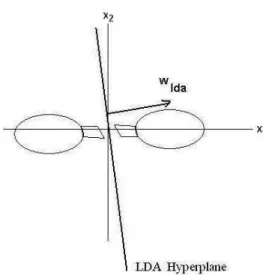
On the other hand, the description of the SVM solu-tion, summarized by expression (2), does not depend on the class distributions, focusing on support vectors which are the observations that lie on the boundary of the mar-gin. In other words, SVM discriminant direction focuses on the data that are most important for classification, but such data are not necessarily the most important ones for extracting discriminant information between the sample groups. Figures 1 and 2 picture these aspects. They show a hypothetical data set composed of two classes and the separating planes obtained respectively by the LDA and SVM methods.
Figure 1 shows the LDA hyperplane which normal di-rection is clearly biased by the class distributions whereas the Figure 2 pictures SVM solution which, according to the optimality criterium behind SVM, searches for the plane that separates the subsets with maximal marging. Figure 1 illustrates the fact that LDA solution is less sen-sitive to the subtleties of group differences found in the frontiers of the classes than SVM which gives a zoom into these subtleties. This is the reason why SVM is more
Figure 1. Hypothetical example: LDA separating hyperplane.
robust nearby the classification boundary of the classes achieving best recognition rates.
However, when considering reconstruction, things be-come different. Let a pointxin the feature space be com-puted by the following expression:
x=x+δ·w, w∈ {wlda,wsvm}, (13)
where δ ∈ ℜ and x is, for instance, the grand mean vector computed by expression (5). The LDA discrimi-nant direction takes into account all the data because it maximizes the between-class separability while minimiz-ing their within-class variability. This can be quantified by expression (12) which shows that LDA tries to col-lapse the classes into single points, their sample group means, as separated as possible. Therefore, when we set
w = wlda in equation (13) we are moving along a
di-rection that represents essentially the difference of the sample means normalized by the spread of the samples on the whole feature space when computing thexpoint. On the other hand, expression (2) computes the SVM dis-criminant direction wsvm through a linear combination
of the support vectors. Therefore, SVM does not take into account the information about the class prototypes and spreads. Consequently, we expect a more informa-tive reconstruction result when w = wldathan the one
obtained by SVM discriminant direction, in terms of ex-tracting group differences. Thus, Figures 1 and 2 are an attempt to represent these aspects in the sense that wlda
is closer thanwsvmto the directiond=x1−x2.
4. D
ISCRIMINANTF
EATURESA
NALYSIS(DFA)
We approach the problem of selecting and recon-structing the most discriminant features as a problem of estimating a statistical linear classifier. Hence, an n -dimensional feature space{x1, x2, ..., xn}is defined and
a training set, consisting ofN measurements, is selected to construct both MLDA and SVM separating hyper-planes. However, we shall emphasize that any separating hyperplane can be used here.
Thus, assuming only two classes to separate, the ini-tial training set is reduced to a data set consisting of N
measurements on only1discriminant feature given by:
˜
y1 = x11w1+x12w2+...+x1nwn, (14)
˜
y2 = x21w1+x22w2+...+x2nwn, ...
˜
yN = xN1w1+xN2w2+...+xN nwn,
where w = [w1, w2, ..., wn]T is the discriminant
direc-tion calculated by either MLDA or SVM approach, and
[xi1, xi2, ..., xin],i= 1, ..., Nare the sample features.
We can determine the discriminant contribu-tion of each feature by investigating the weights [w1, w2, ..., wn]
T
of the corresponding discriminant direction w. Weights that are estimated to be 0 or approximately0have negligible contribution on the dis-criminant scoresy˜idescribed in equation (14), indicating
that the corresponding features are not significant to separate the sample groups. In contrast, largest weights (in absolute values) indicate that the corresponding features contribute more to the discriminant score and consequently are important to characterize the differences between the groups.
Therefore, we select as the most important discrimi-nant features the ones with the highest weights (in abso-lute values), that is,|w1| ≥ |w2| ≥ ...≥ |wn|described
by either the MLDA separating hyperplane
wmlda= arg max w
wTSbw
|wTS∗ ww|
(15)
or the SVM separating hyperplane, as described in equa-tion (2) and repeated here as a reminder,
wsvm= N
i=1
αiyi(xi). (16)
In short, we are selecting among the original features the ones that are efficient for discriminating rather than representing the samples.
Once the statistical linear classifier has been con-structed, we can move along its corresponding discrim-inant direction and extract the group differences captured by the classifier. Therefore, assuming that the spreads of the classes follow a Gaussian distribution and applying limits to the variance of each group, such as±3σi, where σiis the standard deviation of each groupi∈ {1,2}, we
can move alongwmldaandwsvmand perform a
discrim-inant features analysis of the data. Specifically, this map-ping procedure is generated through expression (13), set-tingδ=jσi, wherej∈ {−3,−2,−1,0,1,2,3},x=xi,
and replacingwwithwmldaorwsvm, that is:
xi,j=xi+jσi·w, w∈ {wlda,wsvm}. (17)
5. C
ASES
TUDY1: F
ACEI
MAGESWe present in this section experimental results on face images analysis. These experiments illustrate firstly the reconstruction problem based on the most expressive principal components and then compare the discrimina-tive information extracted by the MLDA and SVM linear approaches. Since the face recognition problem involves small training sets and a large number of features, com-mon characteristics in several pattern recognition applica-tions, and does not require a specific knowledge to inter-pret the differences between groups, it seems an attractive application to investigate and discuss the statistical learn-ing methods studied in this work.
5.1. FACEDATABASE
We have used frontal images of a face database main-tained by the Department of Electrical Engineering of FEI to carry out the experiments. The FEI face database contains a set of face images taken between June 2005 and March 2006 at the Artificial Intelligence Labora-tory in S˜ao Bernardo do Campo, S˜ao Paulo, Brazil, with 14 images for each of 200 individuals - a total of 2800 images. All images are colorful and taken against a white homogenous background in an upright frontal po-sition with profile rotation of up to about 180 degrees. Scale might vary about 10% and the original size of each image is 640x480 pixels. All faces are mainly repre-sented by subjects between 19 and 40 years old with dis-tinct appearance, hairstyle, and adorns. This database is publicly available for download on the following site http://www.fei.edu.br/∼cet/facedatabase.html.
To minimize image variations that are not necessarily related to differences between the faces, we first aligned all the frontal face images to a common template so that the pixel-wise features extracted from the images corre-spond roughly to the same location across all subjects. In this manual alignment, we have randomly chosen the frontal image of a subject as template and the directions of the eyes and nose as a location reference. For imple-mentation convenience, all the frontal images were then cropped to the size of 360x260 pixels and converted to 8-bit grey scale. Since the number of subjects is equal to 200 and each subject has two frontal images (one with a neutral or non-smiling expression and the other with a smiling facial expression), there are 400 images to per-form the experiments.
5.2. PCA RECONSTRUCTIONRESULTS
It is well-known that well-framed face images are highly redundant not only owing to the fact that the im-age intensities of adjacent pixels are often correlated but also because every individual has one mouth, one nose, two eyes, etc. As a consequence, we can apply
dimen-sionality reduction in order to project an input image with
npixels onto a lower dimensional space without signifi-cant loss of information. Principal Components Analysis (PCA) is a feature extraction procedure concerned with explaining the covariance structure of a set of variables through a small number of linear combinations of these variables.
Thus, let anN×ntraining set matrixXbe composed of N input face images withnpixels. This means that each column of matrixXrepresents the values of a par-ticular pixel observed all over theNimages. Let this data matrixXhave covariance matrixSwith respectivelyP
andΛeigenvector and eigenvalue matrices, that is,
PTSP=Λ. (18)
It is a proven result that the set ofm(m ≤n) eigen-vectors ofS, which corresponds to themlargest eigen-values, minimizes the mean square reconstruction error over all choices of morthonormal basis vectors (Fuku-naga, 1990). Such a set of eigenvectors that defines a new uncorrelated coordinate system for the training set matrix
Xis known as the principal components. In the context of face recognition, thosePpca = [p1,p2, ...,pm]
com-ponents are frequently called eigenfaces [29].
As the average face image is ann-dimensional point (n=360x260=93600) that retains all common features from the training sets, we could use this point to under-stand what happens statistically when we move along the principal components and reconstruct the respective co-ordinates on the image space. Analogously to the works by Cootes et al. [6, 5, 7], we have changed the average face image x by reconstructing each principal compo-nent separately using the limits of ±√λi, where λi are
the corresponding largest eigenvalues. Specifically, we setδ = j√λi, withj ∈ {−3,−2,−1,0,1,2,3}, in
ex-pression (13) and replacewwith the principal directions, that is:
xi,j=x+j
λi·pi, i= 1,2, . . . ,7 (19)
where p1,p2. . . ,p7 are the first seven most expressive
principal components.
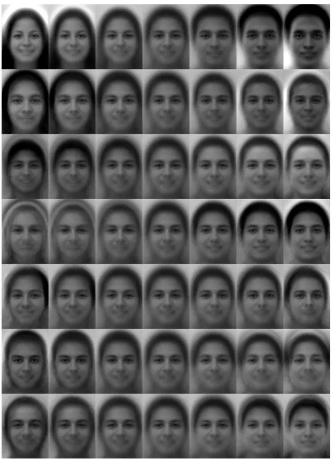
Figure 3. Reconstruction of the PCA most expressive components, i.e., from top to bottom, the first seven principal components with the largest eigenvalues in descending order. Each rowiof images represents the following reconstruction defined by equation (19):
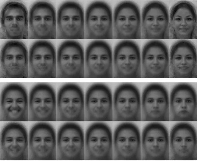
Figure 5. Reconstruction of the discriminant features captured by the MLDA and SVM statistical learning approaches. First two rows represent the gender experiments: MLDA (top) and SVM (bottom). Last two rows correspond to the facial expression experiments: MLDA (top) and SVM (bottom). From left (group 1 of male or smiling samples) to right (group 2 of females or non-smiling samples) each row of images represents the
following reconstruction defined by equation (17):[x1,−3,x1,0,x1,+1,
x1,0+x2,0
2 ,x2,−1,x2,0,x2,+3].
describes some profile changes of the subjects that can-not be characterized as either gender or expression vari-ation. The last two most expressive components capture other variations that are related to male and female differ-ences such as the presence or absence of beard around the cheeks and chin regions.
As we should expect, these experimental results show that PCA captures features that have a considerable vari-ation between all training samples, like changes in illu-mination, gender, and head shape. However, if we need to identify specific changes such as the variation in facial expression solely, PCA has not proved to be a useful so-lution for this problem. As it can be seen in Figure 3, although the fourth principal component models some fa-cial expression variation, this specific variation has been subtly captured by other principal components as well in-cluding other image artifacts. Likewise, as Figure 3 il-lustrates, although the first principal component models
gender variation, other changes have been modeled con-currently, such as the variation in illumination. In fact, when we consider a whole grey-level model without land-marks to perform the PCA analysis, there is no guarantee that a single principal component will capture a specific variation alone, no matter how discriminant that variation might be.
5.3. INFORMATION EXTRACTION AND CLASSIFI
-CATIONRESULTS
female and male images, and their respective frontal smil-ing images. The idea of the first discriminant experiment is to evaluate the statistical learning approaches on a dis-criminant task where the differences between the groups are evident. The second experiment poses an alternative analysis where there are subtle differences between the groups.
Before evaluating the classification performance of the separating hyperplanes, we first analyze the linear discriminant features extracted by the MLDA and SVM statistical learning methods. Since the separating hyper-planes have been calculated on the PCA feature space, DFA can determine the MLDA and SVM discriminant contribution of each pixel on the original image space by multiplyingwmldaandwsvmby the transpose of the
principal components matrixPpca.
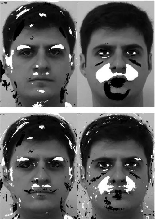
Figure 4 shows the spatial distribution of the discrim-inant pixels extracted by each separating hyperplane su-perimposed on the template image used to align all the frontal faces. We highlight only the pixels which corre-spond to the 5% largest (in absolute values) positive and negative weights. We can see clearly that by exploring the separating hyperplane found by the statistical learning approaches and ranking their most discriminant pixels we are able to identify features that most differ between the group samples, such as: hair, eyebrow, eyes, nose, upper lip, chin and neck for the gender experiments; and eyes, shadow, cheek, upper lip and mouth for the facial expres-sion experiments. As we should expect, changes in facial expression are subtler and more localized than the gen-der ones. Moreover, it is important to note that the dis-criminant features vary depending on the separating hy-perplane used. We observe that the discriminant features extracted by MLDA are more informative and robust for characterizing group-differences than the SVM ones.
Figure 5 summarizes the reconstruction results cap-tured by the multivariate statistical classifiers using all the gender and facial expression training samples. Specif-ically, these images are generated through expression (17), replacing w withwmlda andwsvm. As it can be
seen, both MLDA and SVM hyperplanes similarly ex-tracts the gender group differences, showing clearly the features that mainly distinct the female samples from the male ones, such as the size of the eyebrows, nose and mouth, without enhancing other image artifacts. Look-ing at the facial expression spatial mappLook-ing, however, we can visualize that the discriminative direction found by the MLDA has been more effective with respect to ex-tracting group-differences information than the SVM one. For instance, the MLDA most discriminant direction has predicted facial expressions not necessarily present in our corresponding expression training set, such as the ”def-initely smiling” or may be ”happiness” status and ”defi-nitely non-smiling” or may be ”anger” status represented
respectively by the left most and right most images in the third row of Figure 5.
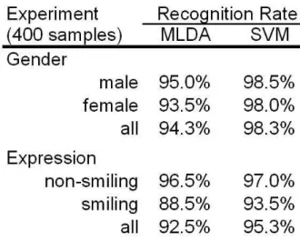
Finally, Table 1 shows the leave-one-out recognition rates of the MLDA and SVM classifiers on the gender and facial expression experiments. As it can be seen, in both experiments SVM achieved the best recognition rates showing higher classification results than the MLDA approach. These results confirm the fact that SVM is a more robust technique for classification than MLDA, as already pointed out in section 3.
Table 1. Classification results of the MLDA and SVM separating hyperplanes.
6. C
ASES
TUDY2: B
REASTL
ESION In [17], authors have proposed an automatic method-ology for breast lesion classification in ultrasound images based on the following five-step framework: (a) Non-extensive entropy segmentation algorithm; (b) Morpho-logical cleaning to improve segmentation result; (c) Ac-curate boundary extraction through level set framework; (d) Feature extraction; (e) SVM non-linear classification using the breast lesion features as inputs.6.1. FIVE-STEPULTRASOUNDFRAMEWORK
corre-(a)
(b)
Figure 6. (a) Original ultrasound benign image; (b) NESRA segmentation.
sponding result after the non-extensive segmentation with the NESRA algorithm (on the bottom). The justification of why using a non-extensive segmentation algorithm for ultrasound images can be found in [17] and references therein.
As described in the framework, in the second step we have used a morphological chain approach in order to ex-tract the region of interest (ROI) from the background. This was accomplished through the following rule. Con-sidering the binary image generated by NESRA (e.g Fig-ure 6-b), letαandβbe the total ROI’s area and the total image area, respectively. Ifα≥ξβan erosion is carried out and ifα≤δβa dilation is performed. Assuming that the ROI has a geometric point near to the image center, we apply a region growing algorithm which defines the final ROI’s boundary. In [17] it was setξ= 0.75andδ= 0.25 to extract most the ROIs. The result of this morphologi-cal rule applied in the image of Figure 6-b is illustrated in Figure 7-a. As it can be seen, the region generated by the morphological chain rule is a coarse representation of the lesion region. Then, we have applied a level set frame-work [17] using as initialization this region’s boundary [19]. The result can be seen in Figure 7-b, which was accomplished with only 10 iterations of the level set ap-proach.
The result of the lesion extraction illustrated in Figure 7 was used as input to calculate the tumor features com-monly used by radiologists in diagnosis. Then, the next step is the feature extraction of the ROI. In the work
pre-(a)
(b)
Figure 7. (a) ROI after morphological step; (b) final ROI after the level set approach.
sented in [17], three radiologists stated five features which have high probability to work well as a discriminator be-tween malignant and benign lesions. Then, we have used these features and tested them in order to achieve the best combination in terms of performance. The feature space has been composed of the following attributes:
• Area (AR): The first feature considered is the lesion area. As indicated by the radiologists, since malig-nant lesions generally have large areas in relation to benign ones, this characteristic might be an impor-tant discriminant feature. We have normalized it by the total image area.
• Circularity (CT): The second characteristic is related to the region circularity. Since benign lesions gen-erally have more circular areas compared with the malignant ones, this can also be a good discrimi-nant feature. Then, we have taken the ROI’s geo-metric center point and compute the distance from each boundary point(xi, yi)to it. We should expect
that malignant lesions tend to have high standard de-viations of the average distances in relation to the benign ones. Also, this feature is normalized by to-tal image area.
as a protuberance between two valleys. The lobe ar-eas are computed and only those greater than10%of the lesion area are considered. This feature is taken as the average area of the lobes. According to the radiologists, we might expect that malignant lesions have higher average area than benign ones.
• Homogeneity (HO): The next feature is related to the homogeneity of the lesion. Malignant lesions tend to be less homogeneous than benign ones. Then, we take the Boltzman-Gibbs-Shannon entropy – taken over the gray scale histogram – relative to the max-imum entropy as the fourth discriminant feature. In this case, we should expect that as higher the relative entropy less homogeneous is the lesion region and, consequently, higher is the chance to be a malign le-sion.
• Acoustic Shadow (AS): The last feature is related with a characteristic called acoustic shadow. In be-nign lesions there are many water particles and, as a consequence, dark areas below such lesions are likely to be detected. On the other hand, when the le-sion is more solid (a malignant characteristic), there is a tendency in forming white areas below it. We have computed the relative darkness between both areas (lesion’s area and area below the lesion) and have taken it as the fifth lesion feature.
These features are the input to a SVM classifier that separates the breast lesions between malignant and benign types. The applied SVM utilizes B-spline as a kernel in its framework. In [17], authors justified the use of a B-Spline as a kernel for the SVM by comparing its perfor-mance with polynomial and exponential kernels. Addi-tionally, in [17], ROC analyzes of several combinations of the five-feature set have been performed to determine the best recognition performance of the framework. Although the experimental results reported in [17] have shown that area, homogeneity, and acoustic shadow gives the best classification rates, no theoretical justification was pre-sented in order to select a specific subset of the origi-nal feature space for optimum information extraction and classification performance.
6.2. INFORMATION EXTRACTION AND CLASSIFI
-CATIONRESULTS
We repeat the same experiments carried out in [17], which have used a 50 pathology-proven cases database (20 benign and 30 malignant) to evaluate our DFA method on the five-step ultrasound framework previously de-scribed. Each case is a sequence of 5 images of the same lesion. Thus, we tested 100 images of benign lesion and 150 of malignant ones, that is, a total of 250 difference case.
Since the SVM separating hyperplane has been calcu-lated on the original feature space, DFA can determine the discriminant contribution of each feature by investigating the weights of the most discriminant direction found by the SVM approach. Table 2 lists the features in decreas-ing order of discriminant power (in absolute values) se-lected by the SVM separating hyperplane using all the samples available. As it can be seen, SVM has selected the AR feature as the most discriminant feature, followed by AS, HO, CT and PT. In other words, we should expect a better performance of the classifier when using, for in-stance, two features only, if we select the pair of features (AR, AS)rather than(CT, P T).
1 Area (AR)
2 Acoustic Shadow (AS) 3 Homogeneity (HO) 4 Circularity (CT) 5 Protuberance (PT)
Table 2. SVM most discriminant features in decreasing order.
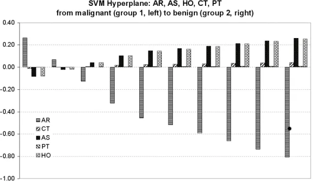
Analogously to the previous face experiments, the other main task that can be carried out by the DFA ap-proach is to reconstruct the most discriminant feature de-scribed by the SVM separating hyperplane. Figure 8 presents the SVM most discriminant feature of the five-feature dataset using all the examples as training samples. It displays the differences on the original feature space captured by the classifier that change when we move from one side (malignant or group 1) of the dividing hyperplane to the other (benign or group 2). Specifically, these vari-ations are generated through expression (17), replacing
wwithwsvm. We can see clearly differences in the AR
as well as AS and HO features. That is, the changes on the AR, AS, and HO features are relatively more signif-icant to discriminate the sample groups than the CT and PT features. Additionally, Figure 8 illustrates that when we move from the definitely benign samples (on the right) to the definitely malign samples (on the left), we should expect an relative increase on the lesion area (AR), and a relative decrease on the acoustic shadow (AS) and homo-geneity (HO) of the lesion. All these results are plausible and provide a quantitative measure to interpreting the dis-criminant importance and variation of each feature in the classification experiments.
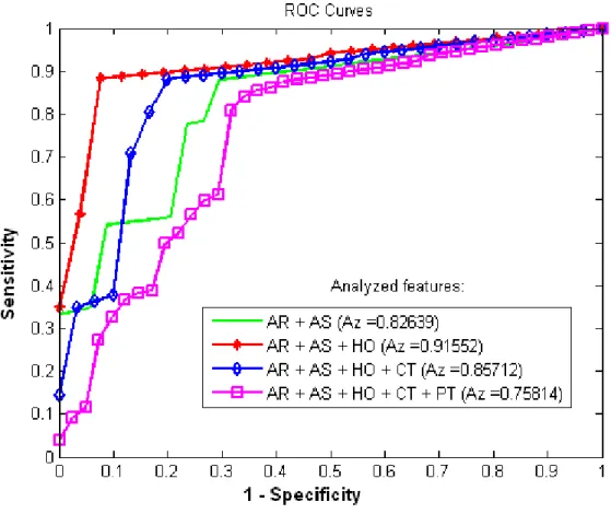
Following the discriminant order and importance sug-gested in Table 2 and Figure 8 respectively, we can guide our classification experiments by combining the features according to those which improve the groups separation. Then, we carried out further classification experiments ac-cording to the following features combination:
1. AR + AS
Figure 8. Reconstruction of the discriminant features captured by the SVM statistical learning approach on the five-step framework. From left (group 1 of malignant samples) to right (group 2 of benign samples) each five-set of clustered bars represents the following reconstruction defined by
equation (17):[x1,−3,x1,−2,x1,−1,x1,0,
x1,0+x2,0
2 ,x2,−1, ,x2,0,x2,+1,x2,+2,x2,+3].
3. AR + AS + HO + CT
4. AR + AS + HO + CT + PT
We have adopted the same cross-validation strategy carried out in [17] to evaluate these classification experi-ments. That is, the ultrasonic images are firstly divided randomly into five groups. We first set the first group as a test set and use the remaining four groups to train the SVM. After training, SVM is then tested on the first group. Then, we set the second group as a testing group and the remaining four groups as training set, and then SVM is tested on the second. This process is repeated until all the five groups have been set in turn as test sets.
In order to evaluate our results, we have used the Re-ceiver Operating Characteristic (ROC) curve, which is a useful graph for organizing classifiers and visualizing their performance. Also, it is the most commonly used tool in medical decision tasks, and in recent years have been used increasingly in machine learning and data min-ing research. A nice recent review and discussion about the ROC analysis can be found in [9]. Briefly, ROC curves are two-dimensional graphs where true positive (TP) rate is visualized on the vertical axis and false posi-tive (FP) rate is visualized on the horizontal axis. As such, a ROC curve tries to show relative tradeoffs between ben-efits (true positives) and costs (false positives) of a mea-suring. Other two indexes are true negative (TN) and false
negative (FN). Under these four indexes, we can set sev-eral other indexes as follows:
• Accuracy =(T P+T N)/(T P+T N+F P+F N) • Sensitivity =T P/(T P +F N)
• Specificity =T N/(T N+F P)
• Positive Predictive Value (PPV) =T P/(T P+F P) • Negative Predictive Value(NPV) =T N/(T N+F N) Together, all these five indexes guarantee a perfect classifier measuring. The commonly strategy is plotting the sensitivity as a function of the (1 - specificity) (see, for instance [9]) as a ROC curve. As larger the area under the ROC curve (that is, Az area), together with high accu-racy, PPV and NPV, better is the classifier performance in terms of separating the sample groups.
Figure 9. ROC curves for different combinations of the discriminant features in SVM classification of breast lesions.
7. C
ONCLUSIONIn this paper, we described and implemented a method of discriminant features analysis based on sample group-differences extracted by separating hyperplanes. This method, called here simply as DFA, is based on the idea of using the discriminant weights given by statistical lin-ear classifiers to select and reconstruct among the original features the most discriminant ones, that is, the original features that are efficient for discriminating rather than representing all samples. The two case studies carried out in this work using face images and breast lesion data sets indicated that discriminant information can be efficiently captured by a linear classifier in the high dimensional original space. In both case studies, the results showed that the DFA approach provides an intuitive interpreta-tion of the differences between the groups, highlighting and reconstructing the most important statistical changes between the sample groups analyzed.
As future works, we can extend the DFA approach to several classes because both MLDA and SVM statistical learning methods used in this work can be generalized to multi-class problems. Additionally, we can perform similar experiments for a general separating hypersurface,
that is, a non-linear discriminant features analysis. In this case, the normal direction changes when we travel along the separating boundary, which may bring new aspects for the reconstruction process.
ACKNOWLEDGMENTS
The authors would like to thank the reviewers for their several comments that significantly improved this work. The authors also would like to thank Leo Leonel de Oliveira Junior for acquiring and normalizing the FEI face database under the grant FEI-PBIC 32-05. The SVM code used in this work is based on the quadratic program-ming solution created by Alex J. Smola. In addition, the authors would like to thank the support provided by PCI-LNCC, FAPESP (grant 2005/02899-4), and CNPq (grants 473219/04-2 and 472386/2007-7).
R
EFERENCES[1] R. Beale and T. Jackson. Neural Computing. MIT Press, 1994.
ma-chines for pattern recognition. Data Mining and Knowledge Discovery, 2(2):121–167, 1998.
[3] W. Chang. On using principal components before separating a mixture of two multivariate normal dis-tributions.Appl. Statist., 32(3):267–275, 1983.
[4] L. Chen, H. Liao, M. Ko, J. Lin, and G. Yu. A new lda-based face recognition system which can solve the small sample size problem.Paterns Recognition, 33:1713–1726, 2000.
[5] T. F. Cootes, G. J. Edwards, and C. J. Taylor. Active appearance models. InECCV’98, pages 484–498, 1998.
[6] T. F. Cootes, C. J. Taylor, D. H. Cooper, and J. Gra-ham. Active shape models- their training and appli-cation.Computer Vision and Image Understanding, 61(1):38–59, 1995.
[7] T. F. Cootes, K.N. Walker, and C.J. Taylor. View-based active appearance models. In 4th Interna-tional Conference on Automatic Face and Gesture Recognition, pages 227–232, 2000.
[8] P.A. Devijver and J. Kittler. Pattern Classification: A Statistical Approach. Prentice-Hall, 1982.
[9] T. Fawcett. An introduction to roc analysis. Pattern Recogn. Lett., 27(8):861–874, 2006.
[10] K. Fukunaga. Introduction to statistical pattern recognition. Boston: Academic Press, second edi-tion, 1990.
[11] A. Gelman and J. Hill. Data Analysis Using Re-gression and Multilevel/Hierarchical Models. Cam-bridge University Press, 2007.
[12] P. Golland, W. Grimson, M. Shenton, and R. Kiki-nis. Detection and analysis of statistical differences in anatomical shape.Medical Image Analysis, 9:69– 86, 2005.
[13] P. Golland, W. Eric L. Grimson, Martha E. Shenton, and Ron Kikinis. Deformation analysis for shape based classification.Lecture Notes in Computer Sci-ence, 2082, 2001.
[14] T. Hastie, R. Tibshirani, and J.H. Friedman. The Elements of Statistical Learning. Springer, 2001.
[15] C. J. Huberty. Applied Discriminant Analysis. John Wiley & Sons, INC., 1994.
[16] I. T. Jolliffe, B. J. T. Morgan, and P. J. Young. A simulation study of the use of principal component in linear discriminant analysis.Journal of Statistical Computing, 55:353–366, 1996.
[17] P. S. Rodrigues, G. A. Giraldi, Ruey-Feng Chang, and J. S. Suri. Non-extensive entropy for cad sys-tems of breast cancer images. In In Proc. of In-ternational Symposium on Computer Graphics, Im-age Processing and Vision - SIBGRAPI’06, Manaus, Amazonas, Brazil, 2006.
[18] B. W. Silverman. Density Estimation for Statistics and Data Analysis. Chapman & Hall/CRC, 1986.
[19] J. S. Suri and R. M. Ragayyan. Recent Advances in Breast Imaging, Mammography and Computer Aided Diagnosis of Breast Cancer. SPIE Press, April 2006.
[20] D. Swets and J. Weng. Using discriminants eigen-features for image retrieval. IEEE Trans. Patterns Anal. Mach Intell., 18(8):831–836, 1996.
[21] C. E. Thomaz, N. A. O. Aguiar, S. H. A. Oliveira, F. L. S. Duran, G. F. Busatto, D. F. Gillies, and D. Rueckert. Extracting discriminative informa-tion from medical images: A multivariate linear ap-proach. In SIBGRAPI’06, IEEE CS Press, pages 113–120, 2006.
[22] C. E. Thomaz, J. P. Boardman, S. Counsell, D.L.G. Hill, J. V. Hajnal, A. D. Edwards, M. A. Ruther-ford, D. F. Gillies, and D. Rueckert. A whole brain morphometric analysis of changes associated with preterm birth. InSPIE International Symposium on Medical Imaging: Image Processing, volume 6144, pages 1903–1910, 2006.
[23] C. E. Thomaz, J. P. Boardman, S. Counsell, D.L.G. Hill, J. V. Hajnal, A. D. Edwards, M. A. Ruther-ford, D. F. Gillies, and D. Rueckert. A multivariate statistical analysis of the developing human brain in preterm infants. Image and Vision Computing, 25(6):981–994, 2007.
[24] C. E. Thomaz, J. P. Boardman, D. L. G. Hill, J. V. Hajnal, D. D. Edwards, M. A. Rutherford, D. F. Gillies, and D. Rueckert. Using a maximum uncer-tainty lda-based approach to classify and analyse mr brain images. InInternational Conference on Medi-cal Image Computing and Computer Assisted Inter-vention MICCAI04, pages 291–300, 2004.
[25] C. E. Thomaz and D. F. Gillies. A maximum un-certainty lda-based approach for limited sample size problems - with application to face recognition. In SIBGRAPI’05, IEEE CS Press, pages 89–96, 2005.
Circuits and Systems for Video Technology, Spe-cial Issue on Image- and Video-Based Biometrics, 14(2):214–223, 2004.
[27] C. E. Thomaz, E. C. Kitani, and D. F. Gillies. A maximum uncertainty lda-based approach for lim-ited sample size problems - with application to face recognition. Journal of the Brazilian Computer So-ciety (JBCS), 12(2):7–18, 2006.
[28] C. E. Thomaz, P. S. Rodrigues, and G. A. Giraldi. Using face images to investigate the differences be-tween lda and svm separating hyper-planes. InII Workshop de Visao Computacional, 2006.
[29] M. Turk and A. Pentland. Eigenfaces for recogni-tion. Journal of Cognitive Neuroscience, 3:71–86, 1991.