1
A Work Project, presented as part of the requirements for the Award of a Master’s Degree in
Economics from NOVA – School of Business and Economics
An impact evaluation of Programa de Apoio à Economia
Local (PAEL) on the water services provided by
municipalities in Portugal
Caroline Isabell Ørvik
Student number: 814
A Project carried out under the supervision of:
Professor Pedro Pita Barros
Professor Steffen Hoernig
2
An impact evaluation of Programa de Apoio à Economia Local (PAEL) on
the water services provided by municipalities in Portugal
1This Work Project evaluates the impact of the arrears program «Local Economy Support
Program» (PAEL), on the water services provided by Portuguese municipalities. The
municipalities entering PAEL had to accept a number of commitments, including increasing
taxes and tariffs. Hence, we want to analyze how this affects the water services provided by
municipalities. We find statistical evidence that PAEL was associated with an increase in water
quality, in a range of values for an increase in water quality of 0.373 to 0.663 (in absolute
terms), from an already high average water quality above 98%.
Keywords;Policy evaluation, Treatment effects, Programa de Apoio à Economia Local (PAEL)
1
I wish to acknowledge that this Work Project is based on the analysis of data generously provided by ERSAR – The Water and Waste Services Regulation Authority in Portugal. I would like to thank Ana Albuquerque and David Alves at ERSAR for providing the
3
1. INTRODUCTION 4
2. PAEL: PROGRAMA DE APOIO À ECONOMIA LOCAL 5
2.1. TARIFF GUIDELINES AND THE NEW TARIFF POLICY 6 2.2. THE ORGANIZATION OF THE WATER AND WASTE SECTOR 8 2.3. MUNICIPALITIES IN PROGRAM 1 OF PAEL 9
3. DATA 10
3.1. DATA COLLECTION 10
3.2. QUALITY INDICATORS 10
3.3. VARIABLES 11
4. METHODOLOGY 12
4.1. DIFFERENCE-IN-DIFFERENCE 13
4.2. DEVELOPMENT IN QUALITY INDICATORS 14
4.3. EQUAL TREND ASSUMPTION 14
5. FIXED EFFECTS MODEL 17
6. RANDOM-EFFECTS MODEL 18
7. FIXED OR RANDOM EFFECTS? 20
7.1. LIMITATIONS OF THE DIFFERENCE-IN-DIFFERENCE APPROACH 21
8. OTHER ESTIMATION METHODS FOR TREATMENT EFFECTS 21
8.1. THE REGRESSION ADJUSTMENT ESTIMATOR 22
9. MATCHING ESTIMATORS 23
9.1. NEAREST NEIGHBOR MATCHING 24
10. CONCLUSION 25
4
1.
Introduction
This Work Project performs an impact evaluation of PAEL; «Programa de Apoio à
Economia Local» (or the Local Economy Support Program) on the water services in the
municipalities in Portugal. PAEL is aimed at reducing debt in the municipalities, regularizing
debt payments and improving fiscal discipline in general. One of the obligations that the
municipalities in the program had to oblige to was to determine the tariffs in the water services
according to the recommendations of ERSAR, the water and waste services regulation authority
in Portugal. ERSAR produces different quality indicators for the water services in
municipalities, and some of these will be used as indicators for the evolution in the quality of
these services. By using different estimation methods, we find statistical evidence that Program
1 of PAEL increased the water quality in the affected municipalities.
The water and waste sector in Portugal has been through a rapid transformation in the last
decades, after a new public policy with a program of reforms was defined in 1993. The new
policy included various components, and among them was the definition of new tariff and tax
policies. In 1993, 81% of the dwellings in mainland Portugal were covered by the public water
supply service, while in 2014 it had increased to 95%. In 1993 only 50% of the dwellings in
mainland Portugal were provided with safe water (as defined by national and European
legislation). In 2014 the corresponding share of safe water was above 98 percent (Baptista
2014). ERSAR 2012 operates with 99-100% safe water as a reference value for good service
quality, 97.50-99% as average quality and any value below this as unsatisfactory.
The paper is organized as follows; section 2 describes PAEL and the intuition behind the
program, in addition to the organization of the water sector in Portugal. Section 3 presents the
data, section 4 describes the methodology and section 5-9 introduces the different estimation
5
2.
PAEL: Programa de Apoio à Economia Local
The arrears program PAEL was approved in August/September 2012 (Law 43/2012, 28
August; Portaria 281-A/2012, 14 September). The Portuguese government implemented the
program as one of several specific measures to improve fiscal discipline in local and regional
governments, and the program is expected to stimulate the local economy by increasing the
liquidity of local suppliers (European Commission 2014). The program included a credit line
of €1 billion to the municipalities, enabling eligible municipalities to establish
medium/long-term loan agreements with the state, to be used to pay municipal debts overdue more than 90
days and short term debt. The loan agreements had to be approved by the respective municipal
assemblies and submitted to Tribunal de Contas2 for approval (European Commission 2012). PAEL was divided into two financing programs, depending on the financial situation the
municipalities were in; Program 1 or Program 2. Program 1 includes municipalities that were
covered by a financial rebalancing plan and were in a situation of structural imbalance at
December 31, 2011. The municipalities in Program 2 had a temporary financial imbalance
(Carvalho et al. 2014). In the last week of 2012 six of the municipalities received a first parcel
of the payment from PAEL (Silva and Buček 2016). In 2013, 90 of the municipalities in the
program received the first parcel of support (PLMJ, 2012). As of 2015 there were 103
municipalities in PAEL. Prior to entry in the program, the municipalities had to present a
financial adjustment plan, which contained a set of specified and quantified measures showing
how the restoration of the financial situation will happen. The municipalities falling under
Program 2 had to present a simplified adjustment program. The adjustment plan should take
into account the following; 1) reduction and rationalization of current and capital expenditure;
2) existence of internal control regulations; 3) optimization of own revenue; 4) intensification
2
6
of the financial adjustment in the municipality the first five years of PAEL (Carvalho et al.
2016).
PAEL involves a number of commitments for the municipalities subject to it. These
commitments are monitored during the execution of the contract, and the municipalities in
Program 1 will have to accept tougher commitments than the municipalities in Program 2.
These conditions include raising fees and tax rates to the maximum (e.g. IMI)3. If the municipalities fail to comply with the obligations they have to agree on, they may be subject to
sanctions, for instance in the form of reduced transfers from PAEL, as the loans are released in
several installments (European Commission 2012). One of the obligations that the
municipalities in program 1 were subject to, was aimed at increasing the cost recovery rate in
the sector of sanitation, water and waste, in order to make the services self-sustainable in the
future. The obligations are defined mainly in paragraph 2 and 3 of article 6 in Law No. 43/2012
of 28 August. Article 6 paragraph 2 states that the municipalities in program 1 of PAEL must
comply with the following: “Determine the prices (tariffs) charged by the municipality in the sanitation, water and waste sectors, in accordance with the recommendations of The Water and Waste Services Regulation Authority in Portugal (ERSAR)”.
2.1. Tariff guidelines and the new tariff policy
The aim of this project is to evaluate how the obligation of following ERSAR’s tariffs
recommendations, affected the quality of the water services provided by municipalities in
Portugal. A part of the program of reforms introduced in 1993 was a new tariff policy for public
water and waste services, aiming at promoting a gradual trend towards cost recovery, so that
the services can be self sustainable. Historically, tariffs have been low, and Portugal has sought
3
7
to evolve from low tariffs to the gradual full cost recovery. The aim is for the water and waste
services end-user tariffs should allow for a growing recovery of economic and financial costs
accruing from the provision of services (ERSAR 2015). ERSAR produces quality indicators
every year, including an indicator named «Coverage of total costs» for the different services,
which represents the ratio between total income and gains and total costs.
In 2012 neither the average monthly drinking water supply service tariffs nor cost
recovery levels differed much among regions. The tariff guidelines on tariff formation for
end-users produced by ERSAR in 2009, states that the tariffs for water and waste services must
comply with the principles established by the Environmental Act, the Water Act, the Economic
and Financial Framework for Water Resources, the General Framework for Waste Resources
and the Local Finances Law, and respect these principles:
1. Cost recovery principle4, meaning that water and waste services should allow an increasing recovery of economic and financial costs of their provision, in order to ensure the quality
of service and the operator’s sustainability and based in an efficiency scenario in order not
to unduly penalize end-users with costs resulting from an inefficient system management;
2. Sustainable use of water resources principle, meaning that the water services tariffs should
contribute to the sustainable management of water resources through the growing
internalization of costs and benefits of their use, penalizing waste and high consumption;
3. Affordability principle, meaning that tariffs should allow for the financial capacity of
end-users, to the extent necessary to guarantee a trend towards universal access to water and
waste services;
4. Principle of user’s interests’ protection, meaning that tariffs should ensure the proper
protection of end-users, avoiding possible dominant position abuses by the operator with
regard to service continuity, quality and costs for end-users on one hand, and with regard
4
8
to their supervision and control mechanisms, on the other hand. These mechanisms become
essential under monopoly situations;
5. The elaboration of the tariffs should avoid cross-subsidization practices among different
services and activities provided by the operators, which occurs when the economic outcome
generated by one or more activities is used to determine another’s price.
Thus, it is likely to believe the aim of increasing the cost recovery rate, would increase the
municipalities revenue, and therefore it could increase the overall quality of the services
provided by the municipalities. Tariffs associated with water sales usually represent the greater
part of a utility’s revenue, and the lack of adequate revenues can prevent water systems from
providing safe, reliable and high-quality water (Water Research Foundation).
2.2. The organization of the water and waste sector
The water and waste sector in Portugal can be divided into two sub-sectors; the water
services sub-sector and the municipal waste sub-sector. The water sector is divided into two
services within the scope of basic sanitation, providing drinking water supply and wastewater
management. This analysis will focus on the drinking water supply5. The drinking water supply retail service is in most cases provided by the municipalities or through municipalized services,
which account for 79% of the existing 260 operators. The supply of drinking water includes the abstraction, treatment, elevation, transport, storage and distribution of water (ERSAR 2015).
The responsibility for the water services is divided between the state and the municipalities in
Portugal. The activities in the water services sub-sector has been classified as bulk and retail,
and the state is responsible for the bulk services and the municipalities for the retail services.
The operator (whether state or municipality) can choose between three different management
5
9
models: direct management, delegation and concession. It is also a possibility to arrange
public-public or public-public-private partnerships in the water sector.
To define whether the water services in a municipality was affected by the municipality
entering PAEL, we need to identify the management model of the municipality. If the
municipality uses a direct management model, this implies that the municipality itself is
responsible for running the water system (ERSAR, 2015). Private concessions are not affected
by the PAEL measure. When these concessions are assigned, the tariffs and the regulation of
the values in coming years are established in the beginning of the concessions.
There are also two municipalities in PAEL where municipal companies are providing the
water services. These are Vizela and Vila Real de Santo António. Anyhow, the municipal
company of Vizela does not run the water system, and will not be included in this analysis. The
water supply services in Vila Real de Santo António are served by the municipal company
VRSA (Sociedade de Gestão Urbana). Since Vila Real de Santo António is the only
municipality in mainland Portugal that entered program 1 of PAEL, that is served by a
municipal company, this municipality will be treated as a member of the control group. The
reasoning behind this is that the local finances law states that all municipal companies that are
not financially sustainable, should be shut down. Thus, it should not be likely that the existing
municipal companies are in financial trouble, even though the municipal companies’ budgets
consolidate with the municipalities accounts.
2.3. Municipalities in Program 1 of PAEL
Program 1 of PAEL concerns municipalities that were covered by a financial rebalancing
plan and that were in a situation of structural imbalance on December 31, 2011. Following are
the municipalities in mainland Portugal in Program 1 where the municipality is responsible for
10
Albufeira (2013), Alfândega da Fé (2013), Alijó (2014), Ansião (2013), Borba (2013), Espinho
(2013), Évora (2013), Freixo de Espada à Cinta (2013), Moimenta da Beira (2013), Mourão
(2013), Nelas (2013) and Seia (2013) (Carvalho et al. 2014).
3.
Data
3.1. Data collection
For this analysis, several water supply quality indicators, as defined by ERSAR, will be
used as variables to indicate the quality of the service. The data is collected from the
municipalities and companies providing water and waste services yearly from 2011 to 2015, by
the Water and Waste Service Regulation Authority (ERSAR) in Portugal. The dataset is a short
unbalanced panel dataset; from 2011 to 2015, including 292 companies/municipalities.
3.2. Quality indicators
The following indicators will be used6, as defined by ERSAR in the «Water and waste service quality assessment guide»:
1) Economic accessibility of the service (%): This indicator is designed to assess the adequacy
of the user integration, in terms of accessibility of the service, with regards to the economic
capacity of households to pay for the service provided by the operator. It is defined as the weight
of the average burden with the water supply service in the average disposable income per
household in the system’s intervention area. An increase in this indicator would imply less
affordable services.
2) Water Quality (%): This indicator is designed to assess the adequacy of the user integration
in terms of the quality of the service provided, with regard to the quality of water supplied by
6
11
the operator. It is defined as the percentage of tests carried out from among those required and
that complied with the parametric values.
3) Coverage of total costs: This indicator is intended to assess the level of sustainability of the
service management in economic and financial terms, with regard to the company’s ability to
generate its own forms of covering the costs arising from its activity. It is defined as the ratio
between the total income and gains and the total spending.
4) Rehabilitation of pipes (%/year): This indicator is designed to assess the level of
sustainability of the service management in terms of infrastructure, with regard to the ongoing
rehabilitation of pipes to ensure their gradual renovation and an acceptable average age of the
network. It is defined as the average annual percentage of abduction and distribution pipes more
than ten years old that were rehabilitated in the last five years.
DESCRIPTIVE STATISTICS
VARIABLES Mean Std. Dev. Min./Max.
Water Quality (1368*) 98.67 1.58 87.57/100
Economic accessibility (1365) 0.44 0.16 0.08/0.98
Coverage of total costs (1204) 0.90 0.44 0.1/7
Rehabilitation of pipes (1074) 1.07 3.40 0/96.97
* The numbers in brackets denotes the number of observations
Table 1: Descriptive statistics of the quality indicators
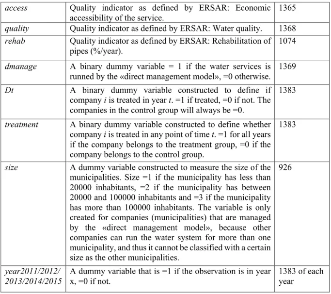
3.3. Variables
Variable name in Stata
Description Number of
observations
companies All municipalities and companies that runs the water system in Portugal. All «companies» are assigned a number, in order to avoid string variables.
1383
year The year of the observation. From 2011-2015. 1383
cover Quality indicator as defined by ERSAR: Coverage of total costs.
12
access Quality indicator as defined by ERSAR: Economic accessibility of the service.
1365
quality Quality indicator as defined by ERSAR: Water quality. 1368
rehab Quality indicator as defined by ERSAR: Rehabilitation of pipes (%/year).
1074
dmanage A binary dummy variable = 1 if the water services is runned by the «direct management model», =0 otherwise.
1369
Dt A binary dummy variable constructed to define if company i is treated in year t. =1 if treated, =0 if not. The companies in the control group will always be =0.
1383
treatment A binary dummy variable constructed to define whether company i is treated in any point of time t. =1 for all years if the company belongs to the treatment group, =0 if the company belongs to the control group.
1383
size A dummy variable constructed to measure the size of the municipalities. Size =1 if the municipality has less than 20000 inhabitants, =2 if the municipality has between 20000 and 100000 inhabitants and =3 if the municipality has more than 100000 inhabitants. The variable is only created for companies (municipalities) that are managed by the «direct management model», because other companies can run the water system for more than one municipality, and thus it cannot be classified with a certain size as the other municipalities.
926
year2011/2012/ 2013/2014/2015
A dummy variable that is =1 if the observation is in year x, =0 if not.
1383 of each year
Table 2: List of variables used in the analysis
4.
Methodology
This project will focus on a quantitative ex post analysis, based on data that was gathered
before, during and after the implementation of PAEL. The ex post policy impact evaluation
measures the actual impact, but may not be able to capture other mechanisms that affects the
outcome. Several estimation methods will be used to estimate the effect on the municipality
water services, of being in Program 1 of PAEL, starting with a description of the
13
4.1. Difference-in-difference
To evaluate the effect of a policy, one of the most frequently used evaluation methods is
the difference (DiD) estimation framework. In essence, the
difference-in-difference estimation is a linear regression that is used in policy analysis, when we want to
analyze the effect of a treatment, the treatment in this case being Program 1 of PAEL. In order
to use this estimation method, the population must be divided into two groups; a treatment
group and a control group. In this case, the treatment group is the 12 municipalities that are
directly responsible for running the water system and were in program 1 of PAEL. We know
that the treatment is not random, but based on the financial situation the municipality is in. The
control group will be all the other municipalities that were either not in program 1 of PAEL or
were in PAEL, but do not run the water system itself. A binary dummy variable, Dit, indicates the treatment of company i in period t. For the control group this variable will always be equal to 0. For a company i that received the first parcel of financial support from PAEL in 2013,
Di2013 =1 and the same in the following years.
This analysis does not follow the standard difference-in-difference method, as the
treatment does not arise at the same time for all the municipalities. All municipalities receive
the treatment in 2013, except one, that receives the treatment in 2014. The
difference-in-difference method compares the changes in outcomes over several points in time, between the
treatment group and the control group, and the difference is calculated between the observed
mean outcomes for the treatment and the control groups, before and after the program was
implemented (Khandker, Koolwal and Samad 2010).
The main assumption of the DiD estimation method is the «Common trend assumption».
This assumption states that if the treated population had not been subjected to the treatment,
both subpopulations would would have experienced the same trends (Lechner 2011). As stated
14
group, the estimated treatment effect can be either invalid or biased. It is not possible to prove
the common trend assumption of natural causes, since only one of the outcomes will be
observed. However, if the outcome time trends are similar before the program was
implemented, this will support the assumption. The process of the difference in difference
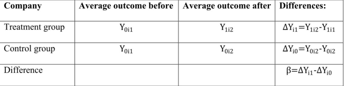
analysis can be presented in a box (table 3), to give a simple overview of the process. β, the treatment effect, is estimated by using the means of the treatment and control group, before and
after the treatment.
Company Average outcome before Average outcome after Differences:
Treatment group Y0i1 Y1i2 ∆Yi1=Y1i2-‐‑Y1i1
Control group Y0i1 Y0i2 ∆Yi0=Y0i2-‐‑Y0i2
Difference β=∆Yi1-‐‑∆Yi0
Table 3: A simple overview of the difference-in-difference analysis
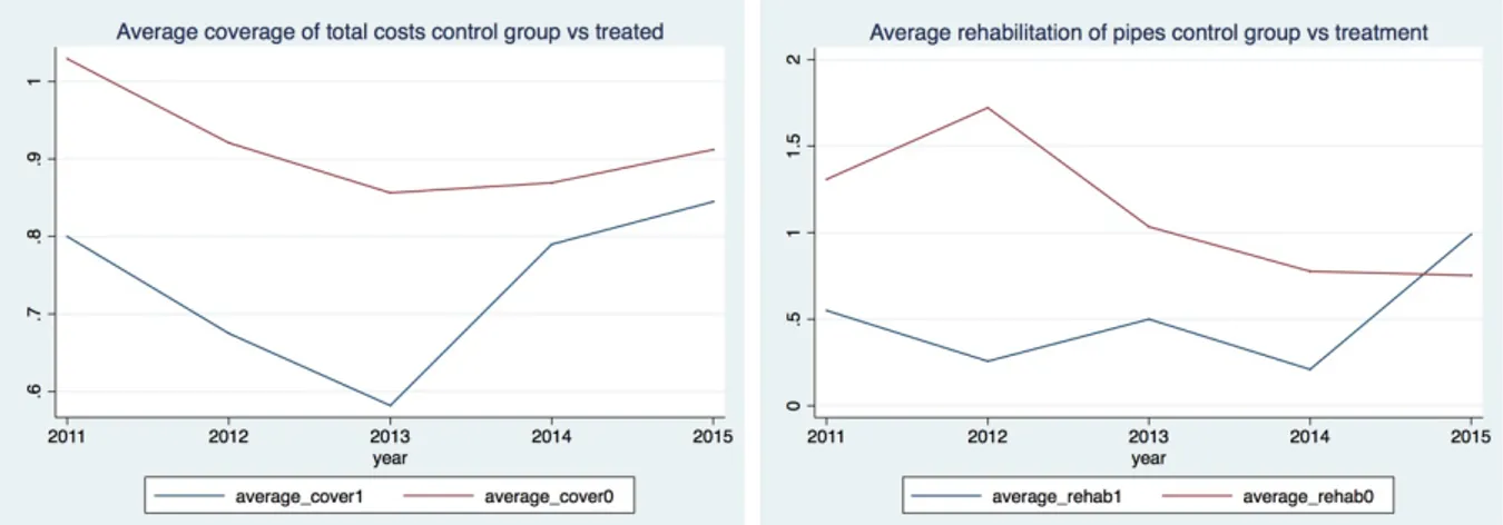
4.2. Development in quality indicators
As presented in graphs 1-4, the control group is at a higher level in 2011 for all the quality
indicators, compared to the treatment group. With the development over time, especially after
2013 (the implementation of PAEL for all but one municipality), the two groups’ averages tend
to converge, and for two indicators the treatment group is at a higher average level in 2015. It
is important to notice that a high level of economic accessibility implies less affordable services.
4.3. Equal trend assumption
11 of the municipalities in the treatment group received their first parcel of payment from
the PAEL program in 2013, and the last municipality received the first parcel in 2014. The data
available is from 2011 until 2015, thus it includes years both prior to and after the treatment
15
common trend assumption would be; before the municipalities enter the treatment, the
municipalities in the treatment group follow the same trend in the quality indicators, as the
control group. As shown in graph 1, 2 and 3, the average of the variable «Economic
accessibility», «Coverage of total costs» and «Water Quality» seems to move in somewhat
similar trends for the two groups until 2013. That is not the case for the variable «Average
rehabilitation of pipes», that is moving in different trends (graph 4). This last variable is not
used in the estimation in the Difference-in-Difference framework, as it does not comply with
the «common trend» requirement. In order to test for the equal trend assumption, we estimate:
Yit=λ0+λ1tDit+εit, where Yit is the dependent variable that we want to test if has similar
time trends for the two groups. The independent variable is time (year). The independent
variable is assigned numerical values, the first year is =1, the second=2, and so forth. Dit=1 if
the observation belongs to the treatment group, and Dit=0 otherwise. According to the common
trend assumption the two groups should have equal trends before the policy is implemented,
thus, if 𝜆0 is similar for the two groups, this will support the assumption of the common trend.
Graph 1: The development of the average water quality in the control group (red) and the treatment
group (blue). Graph 2: The development of the average economic accessibility of the service in the
16
Graph 3: The development of the average coverage of total costs in the control group (red) and the
treatment group (blue). Graph 4: The development of the average rehabilitation of pipes in the control
group (red) and the treatment group (blue).
DESCRIPTIVE STATISTICS Treatment Group
Control Group
Std. Dev. Treatment/
Control
VARIABLES Mean Mean
Water Quality* 98.43 98.68 0.38/0.23
Water Quality 2011 98.03 98.33 2.32/1.77
Water Quality 2012 98.04 98.59 1.91/1.72
Water Quality 2013 98.38 98.66 1.47/1.52
Water Quality 2014 98.78 98.83 1.29/1.49
Water Quality 2015 98.93 98.99 0.54/1.27
*The average water quality for 2011-2015
Table 4: Descriptive statistics of the average quality for the treatment and control group.
The water quality was already at a high level in 2011, and thus it is clear that a possible
increase caused by the implementation of PAEL, can not be very large before it reaches the
highest possible value of 100%. As graph 1-4 exhibits, the gaps between the average of the
quality indicators for the treatment and control group are all smaller in 2015, than before the
17
5.
Fixed effects model
Fixed-effects models are used to analyze the impact of variables that differ over time, and
requires repeated observations from the same individuals. The fixed-effects model explores the
relationship between the independent and the dependent variables within an individual, in this
case the individuals being municipalities. The municipalities can have their own characteristics
that might influence the dependent variable. We assume that something within the individuals
might influence either the independent or the dependent variable, that we need to control for.
The fixed-effects model controls for this correlation, and removes the effect of these
characteristics, to make it possible to estimate the net effect that the independent variables have
on the dependent variable. Another assumption of the fixed-effects model is that the
time-invariant characteristics are unique to the individual, and not correlated with the other
individuals’ characteristics. If a correlation between the error terms is found, a fixed-effects
model is not applicable. To check for this, we will run the Hausman test in section 7, to test a
random effects model against a fixed effects model (Torres-Reyna, 2007).
The fixed effects regression: Yit=β1Xit+αi+uit, where
− αi (i=1,…,n) is the unknown intercept for each individual (n entity-specific intercepts);
− Yit is the dependent variable, where i=individual and t=time;
− Xit represents one independent variable and 𝛽0 is the coefficient for that variable;
− uit is the individual error term.
A fixed effects model with the dependent variable being water quality, estimates the effect of
being in program 1 of PAEL to have a positive effect; an increase of 0.613 in water quality, at
a 5% significance level, which corresponds to an increase of 0,63% from the average water
quality in the treatment group, before the treatment. By adding one covariate (model 2 table 5)
18
(model 3) or yearly dummies (model 4) provides estimates with no statistically significant
results.
VARIABLES (1) (2) (3) (4)
Treatment 0.613** 0.592* 0.528 0.332
(0.270) (0.338) (0.344) (0.337)
Coverage of 0.0538 0.0573 0.0692
total costs (0.113) (0.113) (0.111)
Economic 0.858
accessibility (0.837)
Constant 98.65*** 98.71*** 98.34*** 98.35***
(0.0286) (0.106) (0.380) (0.133)
Observations 1,368 1,204 1,201 1,204
R-squared 0.005 0.004 0.005 0.051
Nr of companies Yearly dummies
292 no
291 no
291 no
291 yes
Standard errors in parentheses *** p<0.01, ** p<0.05, * p<0.1
Table 5: Fixed effects models
In addition to the significant result Program 1 of PAEL has on water quality, we also obtain
an increase in the quality indicator Economics Accessibility of the service, as a result of the
implementation of PAEL. We estimate an increase of 0,059 in the economic accessibility of
the service, from an average of 0.44 in the treatment group before the treatment, that implies
that the water services are less affordable after the treatment7.
6.
Random-effects model
In the random effects models, the variation across the individuals is assumed to be
random, and not correlated with the independent variables in the model, in all time periods (the
past, current and future time periods of the same individual). If the individual effects are
correlated with other variables in the model, the random effect model is not consistent. Thus, it
7
19
is necessary to specify the individual characteristics that might impact the independent
variables. Some variables may not be available and therefore lead to omitted variable bias in
the model (Torres-Reyna, 2007).
The random effects model: Yit=β0Xit+α+uit+εit, where;
− Yit is the dependent variable, where i=individual and t=time.
– uit is the between-individual error and 𝜀9: is the within-individual error.
– Xit represents one independent variable and 𝛽0 is the coefficient for that variable – αi (i=1,…,n) is the unknown intercept for each individual (n entity-specific intercepts)
Using a random effects model checking only the effect of being in program 1 of PAEL
on the dependent variable water quality, estimates an increase of 0,463 in the water quality, at
a significance level of 10 percent (model 1, table 6). By adding one or two more covariates to
the model and using robust standard errors in the regression to control for heteroskedasticity
(model 2 and 3, table 6), we obtain a positive treatment effect, an increase of 0.371 and 0.373
in water quality, at a significance level of 5%. Thus, adding covariates increases the significance
of the treatment variable. This may be because the regression of water quality against only the
treatment does not decrease the variation in water quality around its mean sufficiently, and the
treatment effect is only significant at a 10 percent level. If the variation in water quality is more
associated with a second or third variable, adding these might also change the estimation of the
treatment effect and its significance level, as it does in this context. Adding yearly dummies
(model 4, table 6) provides no statistically significant result for a treatment effect.
The Breusch-Pagan Lagrange Multiplier test helps deciding between a random effects
regression and a simple OLS regression. The null hypothesis is that variances across individuals
20
that a random effects model is appropriate (see table 10 in the Appendix). There is evidence of
significant differences across the municipalities/companies (Torres-Reyna, 2007).
VARIABLES (1) (2) (3) (4)
Treatment 0.463* 0.371** 0.373** 0.160
(0.250) (0.172) (0.173) (0.287)
Coverage of 0.370*** 0.371*** 0.387***
total costs (0.0976) (0.0980) (0.0979)
Economic -0.0506
accessibility (0.425)
Constant 98.68*** 98.39*** 98.42*** 98.08***
(0.0764) (0.116) (0.215) (0.141)
Observations 1,368 1,204 1,201 1,204
Nr. of companies Yearly dummies
292 no
291 no
291 no
291 yes Standard errors in parentheses
*** p<0.01, ** p<0.05, * p<0.1
Table 6: Random effects models
7.
Fixed or random effects?
When choosing between a random effects and a fixed effects estimator the decision
depends on how the time-invariant unobservable variables are related to independent variables
in the model. The use of «random effects» is usually synonymous with no correlation between
the observed explanatory variables and the unobserved effect. Using fixed effects allows for
the independent variables to be correlated with the unobserved effect (Wooldridge 2002). If the
individual effects are correlated with independent variables in the model, a random effects
model is inconsistent. If we are able to ensure that the individual-specific effect is unrelated
with the explanatory variables, a random effects model can be used to make inferences to a
larger population.
This is usually tested by the Durbin-Wu-Hausman test. In essence, the Hausman test
21
and the null hypothesis is that they are not and that the preferred model is a random effects
model and the alternative hypothesis is that a fixed effects model is preferred. In this case, both
a random effects and a fixed effects model estimates a positive treatment effect of Program 1
of PAEL on water quality. Depending on which regressions we use in the Hausman test, it
provides contradicting results. However, running the Hausman test (see table 11-12 in the
Appendix) with the fixed effects regressions that provides a statistically significant positive
treatment effect (model 1 and 2, table 5) against the random effects regressions (model 1 and
2, table 6), both suggests rejecting H0 and thus, choosing a fixed effects model.
7.1. Limitations of the Difference-in-Difference Approach
Even when the trends are parallel before the start of the intervention (the start of the
treatment), bias in the difference in difference (DiD) estimation may still occur. The logic
behind this is that the DiD approach attributes to the treatment any differences in trends between
the treatment and control group, that occur from the time the program is implemented. If any
other factors affect the trends between the two groups, the estimated effect of the program will
be invalid or biased (Gertler et al. 2006). Any factor that affects only the treatment group at the
time of the treatment can invalidate or bias the estimate of the treatment effect. The DiD method
assumes that no such factor is present, though it is by nature not possible to prove. We can only
provide evidence that supports the equal trends assumption, as done in section 4.3.
8.
Other estimation methods for treatment effects
There are several different ways to estimate the average treatment effects based on
observed data, in addition to the difference in difference estimation. Estimating average
treatment effects has become important in the program evaluation literature (Wooldridge 2002).
Treatment effects are introduced by using the potential-outcomes framework. Each individual
22
The potential outcome is the outcome that we do not observe. For instance, if we have an
individual that did not receive the treatment, we observe Y0. Hence, the potential outcome is
Y1. The treatment effects approach seeks to provide a solution to this missing-data problem. We assume that the treatment of individual i only affects the outcome of individual i, which is known as the stable unit treatment value assumption or SUTVA (Wooldridge 2002).
The aim of these estimation methods is, as in the difference-in-difference approach, to
estimate the difference in outcome with and without the treatment. Though now we also
consider that the covariates then can be related to the potential outcomes and the treatment.
Individuals in the treatment group may differ from the individuals in the control group
regarding the covariates, and matching can be effective in removing the possible imbalance in
covariates between the two groups (Rubin 1973). The potential-outcome mean for treatment
level t is the mean potential outcome for the treatment t, thus we never observe both potential outcomes for an individual i. The average treatment effect is the expected treatment effect on a randomly drawn individual from the population, and the average treatment effect for the treated
is the average treatment effect among the individuals that actually received the treatment.
8.1. The regression adjustment estimator
The regression adjustment (RA) uses a regression model to predict potential outcomes
adjusted for other covariates, and models the outcome to account for nonrandom treatment
assignment (Huber and Drukker 2015). The intuition of using the regression adjustment is to
remove covariate imbalance between the treatment and the control groups (Stuart and Rubin
2007). The regression adjustment estimator creates predictions of the outcomes that each
individual would obtain for each treatment level, independent of the treatment the individual
actually received. Averages over all the individuals estimates the potential outcome means for
23
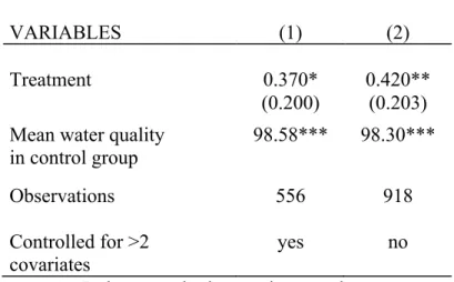
the water quality increased as a result of the municipalities being in program 1 of PAEL. By
controlling for two covariates (model 2, table 7) being in PAEL causes the water quality to
increase by an average of 0.42, from the average of 98.30 in the control group, at a 5%
significance level. By controlling for more covariates (model 1), we estimate an average
increase in the water quality of 0,37 at a 10% significance level. We can express the average
treatment effect on the treated as a percentage of the mean water quality we would have
observed if no municipalities entered PAEL, then we find that being in Program 1 of PAEL
increased the water quality by 0,43% at a significance level of 5%.
VARIABLES (1) (2)
Treatment 0.370* 0.420**
(0.200) (0.203)
Mean water quality in control group
98.58*** 98.30***
Observations
Controlled for >2 covariates
556
yes
918
no
Robust standard errors in parentheses *** p<0.01, ** p<0.05, * p<0.1
Table 7: Regression adjustment estimator
9.
Matching estimators
Matching estimators are often used to estimate treatment effects with lack of experimental
data, and the typical goal is to estimate an average treatment effect (Abadie and Imbens 2011).
The idea behind the matching estimators is to match all treated individuals with the most similar
non-treated individual, and then measure the average difference in the outcome variable
between the treated and non-treated individuals (Khandker, Koolwal and Samad 2010).
The matching method aims at reducing large covariate bias between the treatment group and
24
treatment effects are used to estimate the average treatment effect, or the average treatment
effect on the treated. Given the matched individuals, the treatment effect is estimated as the
difference in outcomes (Imbens & Woolridge 2009).
9.1. Nearest neighbor matching
As there are very few municipalities in program 1 of PAEL (only 12), the nearest neighbor
matching (NNM) estimator can give a more accurate estimate than the difference-in-difference
approach. The NMM method selects a number of control individuals for each of the treated
individuals, and pairs the observation to the closest match(es) in the opposite group (Abadie
and Imbens 2011). When using the NMM, we allow an individual in the treatment group to be
matched with more than one individual from the control group, to find the optimal match. The
nearest neighbor matching for average treatment effects estimates the average treatment effect
on the dependent variable, by comparing observation outcomes between the treated group and
the control group, and provides an estimate of the counterfactual treatment outcome.
VARIABLES (1) (2)
Treatment 0.663** 0.642*
(0.338) (0.330)
Observations Bias adjusted
556 no
556 yes Standard errors in parentheses
*** p<0.01, ** p<0.05, * p<0.1
Table 8: Nearest neighbor matching
By using the variables rehabilitation of pipes, coverage of total costs, economic
accessibility of the service and municipality size as matching variables to define the matching
control observation(s), the treated individuals are matched with at least one, and maximum
three, individuals from the control group (see table 13 and 14 in the Appendix). The
nearest-neighbor matching (model 1, table 8) estimates the average treatment effect on the treated to be
25
Using more than one continuous covariate introduces large-sample bias in the matching,
and in this estimation we use three continuous covariates for matching (rehab, cover & access).
By using the bias-correlated matching estimator we adjust the difference within the matches for
the difference in their covariate values (Abadie et al. 2004). In this case, using the bias-corrected
matching estimator (model 2, table 8) only changes the estimated outcome by a small amount,
but there is now only evidence of a positive effect at a 10% significance level. Hence, the bias
adjustment reduces the significance level, but still estimates a positive treatment effect.
10.
Conclusion
After using different estimation methods to see if, and how, Program 1 of PAEL affected
the water quality, we find evidence that the program had a positive effect on the water quality
in the affected municipalities. The results from the different estimation methods used (table 9),
shows positive results, in a range of values for an increase in water quality from 0.373 to 0.663.
The estimated increase is small, yet these values need to be assessed in the context of an already
high average water quality above 98% in 2011. Hence, it is clear that a possible increase can
not be very high before it reaches the highest possible value of 100% water quality.
Furthermore, the different methods all estimates similar results, and there is statistical evidence
that PAEL was associated with an increase in the water quality in the affected municipalities.
VARIABLES Random
Effects
Fixed Effects
Regression Adjustment
Nearest Neighbor Matching
Treatment 0.373** 0.613** 0.420** 0.642*
(0.173) (0.270) (0.203) (0.330)
Observations 1,201 1,368 918 556
R-squared 0.005
Number of companies
291 292
Robust standard errors in parentheses *** p<0.01, ** p<0.05, * p<0.1
26
11.
References
Abadie, Alberto, David Drukker, Jane Leber Herr and Guido W. Imbens. 2004. ”Implementing matching estimators for treatment effects in Stata”. Stata Journal 4 (3): 290-311.
Abadie, Alberto and Guido W. Imbens. 2011. ”Bias-Corrected Matching Estimators for Average Treatment Effects”. In Journal of Business & Economic Statistic 29 (1): 1-11.
Baptista, Jaime M. 2014. The Regulation of Water and Waste Services – An Integrated Approach (RITA-ERSAR). London: IWA Publishing.
Carvalho, João, Maria José Fernandes, Pedro Camões and Susane Jorge. 2014. Anuàrio Financeiro dos Municípios Portugueses 2013. Accessed September 2016.
http://pt.calameo.com/read/0003249818830e99d8443
Carvalho, João, Maria José Fernandes, Pedro Camões and Susane Jorge. 2016. Anuàrio Financeiro dos Municípios Portugueses 2015. Accessed November 2016.
http://pt.calameo.com/read/000324981f43166e424bc
ERSAR. 2009. ERSAR recommendation nr. 01/2009: Tariff formation for end-users of drinking water supply, urban wastewater and municipal waste management services («Tariff guidelines»). ERSAR – The Water and Waste Service Regulation Authority: Lisbon.
ERSAR. 2012. ”Water and waste service quality assessment guide - 2nd generation of the assessment system”. ERSAR – The Water and Waste Service Regulation Authority/LNEC: Lisbon.
ERSAR. 2015. Annual report on water and waste services in Portugal (2013) – Executive Summary. ERSAR – The Water and Waste Service Regulation Authority: Lisbon.
European Commission. 2012. “The Economic Adjustment Programme for Portugal.” http://ec.europa.eu/economy_finance/publications/occasional_paper/2012/pdf/ocp111_en.pdf European Commission. 2014. “European Economy – The Economic Adjustment Programme for Portugal”. Accessed October 15.
http://ec.europa.eu/economy_finance/publications/occasional_paper/2014/pdf/ocp202_en.pdf Gertler, Paul J., Sebastian Martinez, Patrick Premand, Laura B. Rawlings, Christel M. J. Vermeersch. 2010. Impact Evaluation in Practice. Washington D.C., World Bank.
Huber, Chuck and David Drukker. 2015. Introduction to treatment effects in Stata: Part 1. Accessed October 2016. http://blog.stata.com/2015/07/07/introduction-to-treatment-effects-in-stata-part-1/ Imbens, Guido W. and Jeffrey M. Wooldridge. 2009. “Recent Developments in the Econometrics of Program Evaluation”. Journal of Economic Literature, 47(1): 5-86.
Khandker, Shahidur R., Gayathri B. Koolwal and Hussain A. Samad. 2010. Handbook on impact evaluation: quantitative methods and practices. World Bank Publications: Washington D.C.
Lechner, Michael. 2011. The Estimation of Causal Effects by Difference-in-Difference Methods. Foundations and Trends in Econometrics, 4(3): 165-224.
PLMJ. 2012. Nota Informativa: Programa de Apoio à Economia Local. PLMJ.
Rubin, Donald B. 1973. “The Use of Matched Sampling and Regression Adjustment to Remove Bias in Observational Studies” in Biometrics 29 (1):185-203.
Silva, Carlo Nunes and Ján Buček. 2016. Local Government and Urban Governance in Europe. Springer
International Publishing: Switzerland.
Stuart, Elizabeth A. and Donald B. Rubin. 2007. “Best Practices in Quasi-Experimental Designs: Matching methods for causal inference”. In Quantitative Social Science, edited by J. Osborne, p. 155-176. Sage Publications: Thousand Oaks, CA.
Torres-Reyna, Oscar. 2007. Panel Data Analysis: Fixed and Random Effects using Stata. Princeton University. Accessed October 2016. https://www.princeton.edu/~otorres/Panel101.pdf
Water Research Foundation. Fact sheet: An Updated Approach to Water Revenue. Accessed January
2017. http://www.waterrf.org/knowledge/utility-finance/FactSheets/UtilityFinance-Revenue-FactSheet.pdf