Work Project: An impact evaluation of Programa de Apoio à Economia
Local (PAEL) on the water services provided by municipalities in Portugal
Caroline Isabell Ørvik
1. DETAILS AND INFORMATION 3
TABLE 1:CALCULATIONS OF QUALITY INDICATORS 3
TABLE 2:DRINKING WATER SUPPLY SERVICES 4
TABLE 3:COST RECOVERY PRINCIPLE 4
2. DESCRIPTIVE STATISTICS 5
TABLE 4:QUALITY INDICATORS 5
TABLE 5:WATER QUALITY 5
TABLE 6:REHABILITATION OF PIPES 6
TABLE 7:ECONOMIC ACCESSIBILITY OF THE SERVICE 6
TABLE 8:COVERAGE OF TOTAL COSTS 6
3. OUTPUT TABLES 7
TABLE 9:FIXED EFFECTS MODEL TO CHECK FOR CHANGE IN ECONOMIC ACCESSIBILITY 7
TABLE 10:BREUSCH-PAGAN LAGRANGE MULTIPLIER 7
TABLE 11:HAUSMAN TEST 7
TABLE 12:HAUSMAN TEST 8
TABLE 13:NEAREST NEIGHBOR MATCHING 8
TABLE 14:NEAREST NEIGHBOR MATCHING WITH BIAS ADJUSTMENT 8
1.
Details and information
Table 1: Calculations of quality indicators
Definitions of the calculations of quality indicators and reference values for the level of service quality, produced by ERSAR. Source: ”Water and waste service quality assessment guide - 2nd generation of the assessment system” – ERSAR 2012.
Indicator Definition of how the indicator is
calculated Economic accessibility (%):
It is defined as the weight of the average burden with the water supply service in the average disposable income per household in the system’s intervention area.
AA02ab = dAA52ab / dAA53ab * 100 Where dAA52ab = average cost of the water supply service (€/year) and dAA53ab = average disposable household income (€/year).
Reference values for:
Good service quality: [0; 0.50] Average service quality: ]0.50; 1,00] Unsatisfactory service quality: ]1,00; +∞[
Water quality (%):
It is defined as the percentage of tests carried out from among those required and that complied with the parametric values.
AA04ab = (dAA25ab / dAA23ab) * (dAA22ab / dAA24ab) * 100
Where dAA22ab = tests carried out on the quality of water for human consumption, from among those required by law
(No./year), dAA23ab = tests carried out on the water quality (No./year), dAA24ab = tests required on the water quality (No./year) and dAA25ab = conformity of water tests (No./year).
Reference values for:
Good service quality: [99.00; 100,00] Average service quality: [97.50; 99,00[ Unsatisfactory service quality: [0.00; 97.50[
Coverage of total costs:
It is defined as the ratio between the total income and gains and the total spending.
Ratio between total income and gains and total costs.
AA06ab = dAA50ab / dAA51ab
Where dAA50ab = total income and gains (€/year) and dAA51ab = total costs (€/year)
Reference values for:
Good service quality: [1.0; 1.1]
Average service quality: [0.9; 1.0[or]1.1; 1.2]
pipes more than ten years, old that were rehabilitated in the last five years.
AA10ab = dAA32ab / dAA31ab * 100/5 Where dAA31ab = average length of pipes (km) and dAA32ab = pipes rehabilitated in the last five years (km)
References values for:
Good service quality: [1.0; 4.0]
Average service quality: [0.8; 1.0] or [4.0; 100]
Unsatisfactory service quality: [0.0; 0.8]
Table 2: Drinking water supply services
The drinking water supply services in Portugal includes the following services:
Source: ERSAR 2015: Annual report on water and waste services in Portugal (2013) – Executive Summary
1) Extraction of water from surface or groundwater sources
2) Correction of physical, chemical and microbiological characteristics of water in order to make it fit for human consumption
3) Elevation of water in order for it to circulate under pressure and to enable it to overcome terrain barriers
4) Transport of treated water from the production zone to consumption areas 5) Storage of treated water in such a way as to ensure continuity of supply
6) Water distribution in sufficient quantity and adequate pressure for users’ needs
Table 3: Cost recovery principle
In accordance with the cost recovery principle, tariffs of water and waste services must comply with the provisions of Article 82 of the Water Act, and consider the recovery of the following costs
a) Reintegration and amortization, on time and according to the relevant accounting practices, of the value of the assets allocated to service provision, resulting from investments made with the implementation, maintenance, modernization, rehabilitation or replacement of infrastructure, equipment or resources assigned to the system. b) Operating costs of the operator, including those incurred in the acquisition of materials
and supplies, transactions with the other operators, outsourced services, including the values resulting from the allocation of costs incurred with activities and shared means with other services provided by the operator, or in the salaries of their staff;
c) Financial costs attributable to financing the services and, when applicable, the appropriate return on capital invested by the operator;
2.
Descriptive Statistics
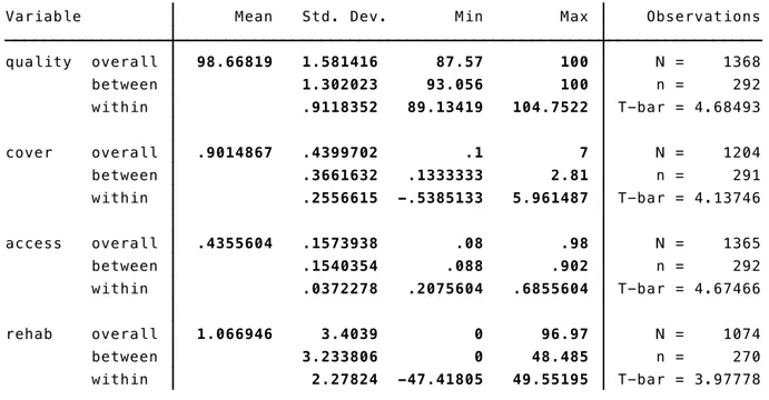
Table 4: Quality Indicators
Descriptive statistics of the quality indicators used in the analysis.
Table 5: Water Quality
Detailed descriptive statistics of the variable «Water Quality»:
within 2.27824 -47.41805 49.55195 T-bar = 3.97778 between 3.233806 0 48.485 n = 270 rehab overall 1.066946 3.4039 0 96.97 N = 1074
within .0372278 .2075604 .6855604 T-bar = 4.67466 between .1540354 .088 .902 n = 292 access overall .4355604 .1573938 .08 .98 N = 1365
within .2556615 -.5385133 5.961487 T-bar = 4.13746 between .3661632 .1333333 2.81 n = 291 cover overall .9014867 .4399702 .1 7 N = 1204
within .9118352 89.13419 104.7522 T-bar = 4.68493 between 1.302023 93.056 100 n = 292 quality overall 98.66819 1.581416 87.57 100 N = 1368 Variable Mean Std. Dev. Min Max Observations
99% 100 100 Kurtosis 10.74586 95% 100 100 Skewness -2.239503 90% 100 100 Variance 2.500876 75% 99.78 100
Largest Std. Dev. 1.581416 50% 99.24 Mean 98.66819 25% 98.04 89.01 Sum of Wgt. 1,368 10% 96.61 88.93 Obs 1,368 5% 95.55 88.3
1% 93.24 87.57 Percentiles Smallest
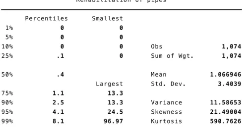
Table 6: Rehabilitation of Pipes
Detailed descriptive statistics of the variable «Rehabilitation of pipes»
Table 7: Economic Accessibility of the Service
Detailed descriptive statistics of the variable «Economic accessibility of the service»
Table 8: Coverage of Total Costs
Detailed descriptive statistics of the variable «Coverage of total costs»
99% 8.1 96.97 Kurtosis 590.7626 95% 4.1 24.5 Skewness 21.49004 90% 2.5 13.3 Variance 11.58653 75% 1.1 13.3
Largest Std. Dev. 3.4039 50% .4 Mean 1.066946 25% .1 0 Sum of Wgt. 1,074 10% 0 0 Obs 1,074 5% 0 0
1% 0 0 Percentiles Smallest
Rehabilitation of pipes
99% .84 .98 Kurtosis 2.911562 95% .7 .95 Skewness .3494403 90% .64 .93 Variance .0247728 75% .54 .93
Largest Std. Dev. .1573938 50% .43 Mean .4355604 25% .32 .09 Sum of Wgt. 1,365 10% .24 .09 Obs 1,365 5% .18 .08
1% .13 .08 Percentiles Smallest
Economic accessibility
99% 2.02 7 Kurtosis 39.40249 95% 1.5 4.9 Skewness 3.274195 90% 1.3 3.2 Variance .1935738 75% 1.1 2.9
Largest Std. Dev. .4399702 50% .9 Mean .9014867 25% .6 .1 Sum of Wgt. 1,204 10% .4 .1 Obs 1,204 5% .3 .1
1% .2 .1 Percentiles Smallest
3.
Output tables
The following tables are output tables from Stata, providing evidence of the results described in the Work Project.
Table 9: Fixed effects model to check for change in Economic Accessibility
We run a fixed effects regression model with the quality indicator Economic Accessibility of the Service being the dependent variable, and find that the treatment effect was an increase of 0,059. This implies that the water supply service as a weight of the burden in the average disposable income per household has increased, thus it implies a less affordable service.
(1)
VARIABLES Access
Treatment 0.0590***
(0.0109)
Constant 0.434***
(0.00116)
Observations 1,365
Number of companies 292
R-squared 0.027
Standard errors in parentheses *** p<0.01, ** p<0.05, * p<0.1
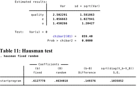
Table 10: Breusch-Pagan Lagrange Multiplier
Table 11: Hausman test
Prob > chibar2 = 0.0000 chibar2(01) = 859.40 Test: Var(u) = 0
u 1.450266 1.20427 e 1.056663 1.027941 quality 2.502291 1.581863 Var sd = sqrt(Var) Estimated results:
quality[companynum,t] = Xb + u[companynum] + e[companynum,t] Breusch and Pagan Lagrangian multiplier test for random effects
B = inconsistent under Ha, efficient under Ho; obtained from xtreg b = consistent under Ho and Ha; obtained from xtreg startprogram .6127778 .4634018 .149376 .1035852 fixed random Difference S.E.
(b) (B) (b-B) sqrt(diag(V_b-V_B)) Coefficients
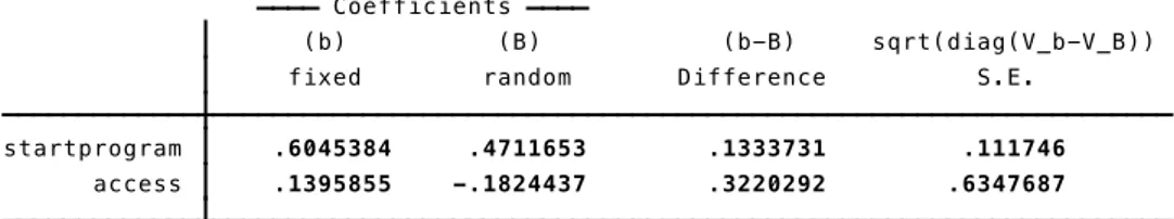
Table 12: Hausman test
Hausman test with more covariates:
Table 13: Nearest Neighbor Matching
Table 14: Nearest Neighbor Matching with bias adjustment Prob>chi2 = 0.2920
= 2.46
chi2(2) = (b-B)'[(V_b-V_B)^(-1)](b-B) Test: Ho: difference in coefficients not systematic
B = inconsistent under Ha, efficient under Ho; obtained from xtreg b = consistent under Ho and Ha; obtained from xtreg access .1395855 -.1824437 .3220292 .6347687
startprogram .6045384 .4711653 .1333731 .111746
fixed random Difference S.E.
(b) (B) (b-B) sqrt(diag(V_b-V_B)) Coefficients
(1 vs 0) .6634 .3381163 1.96 0.050 .0007043 1.326096
startprogram ATET
quality Coef. Std. Err. z P>|z| [95% Conf. Interval] AI Robust
Distance metric: Mahalanobis max = 3
Outcome model : matching min = 1
Estimator : nearest-neighbor matching Matches: requested = 1
Treatment-effects estimation Number of obs = 556
. teffects nnmatch (quality rehab cover access size) (startprogram), atet
(1 vs 0) .6421438 .3296163 1.95 0.051 -.0038922 1.28818 startprogram
ATET
quality Coef. Std. Err. z P>|z| [95% Conf. Interval] AI Robust
Distance metric: Mahalanobis max = 3 Outcome model : matching min = 1 Estimator : nearest-neighbor matching Matches: requested = 1 Treatment-effects estimation Number of obs = 556
4.
Do file from Stata
//Do File for the Work Project at Nova SBE by Caroline Isabell Ørvik #814
use "/Users/carolineorvik/Desktop/Dataset PAEL January2017.dta"
//Set the panel variables (first the panel identifier, then the time identifier) xtset companies year
// Create yearly dummies gen year2011=1 if year==2011 gen year2012=1 if year==2012 gen year2013=1 if year==2013 gen year2014=1 if year==2014 gen year2015=1 if year==2015
replace year2011=0 if year2011!=1 replace year2012=0 if year2012!=1 replace year2013=0 if year2013!=1 replace year2014=0 if year2014!=1 replace year2015=0 if year2015!=1
//To check the Common trend assumption:
//Create mean of variable if/if not in treatment group at any point in time, by year egen average_quality1 = mean(quality) if treatment==1, by (year)
egen average_quality0 = mean(quality) if treatment==0, by (year) egen average_access1 = mean(access) if treatment==1, by (year) egen average_access0 = mean(access) if treatment==0, by (year) egen average_cover1 = mean(cover) if treatment==1, by (year) egen average_cover0 = mean(cover) if treatment==0, by (year) egen average_rehab1 = mean(rehab) if treatment==1, by (year) egen average_rehab0 = mean(rehab) if treatment==0, by (year)
//Average of water quality for treatment group post treatment: egen avgq_post1 = mean(quality) if Dt==1 & treatment==1
//Average of water quality for treatment group pre treatment: egen avgq_pre1 = mean(quality) if Dt==0 & treatment==1
//Average water quality for control group pre treatment:
egen avgq_pre0 = mean(quality) if treatment==0 & year<=2013
//Average quality for control group post treatment:
egen avgq_post0 = mean(quality) if treatment==0 & year>=2013
xtreg quality Dt cover i.year, fe xtreg access Dt, fe
//Test for heteroskedasticity for the fixed effects model (userwritten command) xtreg quality startprogram, fe
xttest3
//Random Effects Model xtreg quality Dt, re
xtreg quality Dt cover, re robust xtreg quality Dt access cover, re robust xtreg quality Dt cover i.year, re robust
//Breusch and Pagan Lagrangian multiplier test (LM) for random effects (userwritten command)
xttest0
//Hausman test to check random vs fixed effects, model with one covariates xtreg quality Dt access, fe
estimates store fixed xtreg quality Dt access, re estimates store random hausman fixed random
//Hausman test to check random vs fixed effects, model with two covariates xtreg quality Dt access cover, fe
estimates store fixed
xtreg quality Dt access cover, re estimates store random
hausman fixed random
//Regression Adjustment estimator
teffects ra (quality rehab cover access size) (Dt), atet teffects ra (quality access size) (Dt), atet
//To express the ATET as a percentage of the mean water quality without treatment teffects ra (quality access size) (Dt), coeflegend atet
nlcom _b[ATET:r1vs0.Dt] / _b[POmean:0.Dt]
//Nearest Neighbor Matching
teffects nnmatch (quality rehab cover access size) (Dt), atet