UNIVERSIDADE FEDERAL DE SÃO CARLOS CENTRO DE CIÊNCIAS EXATAS E TECNOLOGIA
PROGRAMA INTERINSTITUCIONAL DE PÓS-GRADUAÇÃO EM ESTATÍSTICA UFSCar-USP
Marco Henrique de Almeida Inacio
Comparing two populations using Bayesian Fourier series density estimation
Dissertação apresentada ao Departamento de Estatística – Des/UFSCar e ao Instituto de Ciências Matemáticas e de Computação – ICMC- USP como parte dos requisitos para obtenção do título de Mestre em Estatística - Programa Interinstitucional de Pós-Graduação em Estatística UFSCar-USP.
Orientador: Prof. Dr. Rafael Izbicki
ACKNOWLEDGEMENTS
First of all, I would like to say thanks to my parents Nivaldo and Claúdia and my brother João Pedro.
Then to my advisor Rafael Izbicki and to professor Luis Ernesto Bueno Salasar (especially for the help with the introduction of chapter2) for their really amazing help and dedication to this work.
And then to professors José Galvão Leite, Rafael Stern, Luís Gustavo Esteves, Gustavo Henrique de Araújo Pereira, Marcio Alves Diniz, Adriano Kamimura Suzuki, Sandro Gallo, Ricardo Sandes Ehlers, the professors of the evaluation board, the DE/UFSCar graduation secretary Izabel Araujo, and the members of Stan development team.
I would also like to give my acknowledgments to the financial support of CAPES and our nation’s citizens, and hope that the present work will be useful to achieve common good.
RESUMO
INACIO, M. H. DE A. Comparação de duas populações utilizando estimação bayesiana de densidades por séries de Fourier. 2017. 56p. Master dissertation (Master student joint Graduate Program in Statistics DEs-UFSCar/ICMC-USP) – Instituto de Ciências Matemáticas e de Computação, Universidade de São Paulo, São Carlos – SP, 2017.
Dadas duas amostras de duas populações, pode-se questionar o quão parecidas as duas popula-ções são, ou seja, o quão próximas estão suas distribuipopula-ções de probabilidade. Para distribuipopula-ções absolutamente contínuas, uma maneira de mensurar a proximidade dessas populações é uti-lizando uma medida de distância (métrica) entre as funções densidade de probabilidade (as quais são desconhecidas, em virtude de observarmos apenas as amostras). Nesta dissertação, utilizamos a distância quadrática integrada como métrica. Para mensurar a incerteza da distância quadrática integrada, primeiramente modelamos a incerteza sobre cada uma das funções densi-dade de probabilidensi-dade através de uma método bayesiano não paramétrico. O método consiste em estimar a função de densidade de probabilidade f (ou seu logaritmo) usando séries de Fourier
{φ0,φ1, ...,φI}. Atribuir uma distribuição a priori para f é então equivalente a atribuir uma distribuição a priori aos coeficientes dessa serie. Utilizamos a priori sugerida em Scricciolo (2006) (priori de sieve), a qual não coloca uma priori somente nesses coeficientes, mas também no próprioI, de modo que, na realidade, trabalhamos com uma mistura bayesiana de modelos de dimensão finita. Para obter amostras a posteriori dessas misturas, marginalizamos o parâmetro (discreto) de indexação de modelos, I, e usamos um software estatístico chamado Stan. Concluí-mos que o método bayesiano de séries de Fourier tem boa performance quando comparado ao de estimativa de densidade kernel, apesar de ambos os métodos frequentemente apresentarem problemas na estimação da função de densidade de probabilidade perto das fronteiras. Por fim, mostramos como a metodologia de series de Fourier pode ser utilizada para mensurar a incerteza a cerca da similaridade de duas amostras. Em particular, aplicamos este método a um conjunto de dados de pacientes com doença de Alzheimer.
ABSTRACT
INACIO, M. H. DE A.Comparing two populations using Bayesian Fourier series density estimation. 2017. 56p. Master dissertation (Master student joint Graduate Program in Statistics DEs-UFSCar/ICMC-USP) – Instituto de Ciências Matemáticas e de Computação, Universidade de São Paulo, São Carlos – SP, 2017.
Given two samples from two populations, one could ask how similar the populations are, that is, how close their probability distributions are. For absolutely continuous distributions, one way to measure the proximity of such populations is to use a measure of distance (metric) between the probability density functions (which are unknown given that only samples are observed). In this work, we work with the integrated squared distance as metric. To measure the uncertainty of the squared integrated distance, we first model the uncertainty of each of the probability density functions using a nonparametric Bayesian method. The method consists of estimating the probability density function f (or its logarithm) using Fourier series{φ0,φ1, ...,φI}. Assigning a prior distribution to f is then equivalent to assigning a prior distribution to the coefficients of this series. We used the prior suggested byScricciolo(2006) (sieve prior), which not only places a prior on such coefficients, but also onIitself, so that in reality we work with a Bayesian mixture of finite dimensional models. To obtain posterior samples of such mixture, we marginalize out the discrete model index parameter I and use a statistical software called Stan. We conclude that the Bayesian Fourier series method has good performance when compared to kernel density estimation, although both methods often have problems in the estimation of the probability density function near the boundaries. Lastly, we showed how the methodology of Fourier series can be used to access the uncertainty regarding the similarity of two samples. In particular, we applied this method to dataset of patients with Alzheimer.
LIST OF FIGURES
Figure 1 – Plot of some of the components of Fourier series. . . 27
Figure 2 – Plots of the average estimated density using Fourier series for low values ofI. 37 Figure 3 – Plots of the average estimated density using Fourier series for high values ofI. 38 Figure 4 – Average estimated density with data from true model 1. . . 39
Figure 5 – Average estimated density with data from true model 2. . . 40
Figure 6 – Average estimated density with data from true model 3. . . 41
Figure 7 – Estimated mean squared error using data from true model 1. . . 41
Figure 8 – Estimated mean squared error using data from true model 2. . . 42
Figure 9 – Estimated mean squared error using data from true model 3. . . 42
Figure 10 – Plot ofP(M(f1,f2)<ε|D1,D2)againstε. . . . . 44
Figure 11 – Plot ofP(M(f1,f2)<ε|D1,D2)againstε. . . 44
Figure 12 – Probability that the integrated squared distance of thePDFs of two samples is less thanε. . . 46
Figure 13 – Probability that the integrated squared distance of thePDFs of two samples is less thanε. . . 46
Figure 14 – Probability that the integrated squared distance of thePDFs of two samples is less thanε. . . 47
Figure 15 – Probability that the integrated squared distance of thePDFs of two samples is less thanε. . . 48
Figure 16 – Probability that the integrated squared distance of thePDFs of two samples is less thanε. . . 49
Figure 17 – Probability that the integrated squared distance of thePDFs of two samples is less thanε. . . 50
Figure 18 – Plots of the average estimated density using Fourier series with real data . . 51
LIST OF TABLES
Table 1 – Description of the models used to generate data (true models) . . . 35 Table 2 – Estimated mean squared error and mean absolute error for 3 different data
LIST OF ABBREVIATIONS AND ACRONYMS
HMC Halmiltonian Monte Carlo KDE kernel density estimation MAE mean absolute error
MCMC Markov Chain Monte Carlo MSE mean squared error
NUTS No-U-Turn Sampler
CONTENTS
1 INTRODUCTION . . . 23
2 NONPARAMETRIC DENSITY ESTIMATION VIA FOURIER SE-RIES . . . 25
2.1 Frequentist Inference . . . 26
2.2 Bayesian Inference . . . 28
3 HMC, NUTS AND STAN. . . 31
3.1 Stan and discrete parameters . . . 32
4 A SIMULATION STUDY TO ASSESS THE PERFORMANCE OF THE METHOD . . . 35
5 TWO-SAMPLE SIMILARITY ANALYSIS . . . 43
5.1 Simulation study for samples from the same population . . . 45
5.2 Simulation study for samples from the different populations . . . . 47
5.3 An example of two-sample similarity analysis with real data . . . 49
6 CONCLUSION . . . 53
23
CHAPTER
1
INTRODUCTION
Given two samples D1 and D2 from two (possibly different) populations, one could
question how similar the populations are, that is, how close are the probability distributions from which each sample came from.Soriano(2015) andHolmeset al.(2015) among others have
addressed that question by developing methods to do Bayesian nonparametric hypothesis tests via Bayes Factor.
In this dissertation, on the other hand, we propose a different approach that is promising in its intuitiveness: for absolutely continuous distributions on [0,1], one way to measure the proximity of such populations, is to use a measure of distance (metric) between the probability density function (PDF) f1of the first distribution and thePDF f2of the second. In this dissertation,
we’ll work with what we called integrated squared distance:
M(f1,f2) =
Z 1
0 (f1(y)− f2(y))
2dy (1.1)
However, to measure the posterior uncertainty ofM(f1,f2), we first need to measure the
posterior uncertainty of f1 and f2, driving us towards a problem of density estimation which
is among the most significant problems in Statistics. Thanks to the abundance of data in many applications, today there is a great emphasis on nonparametric methods. In particular, Bayesian nonparametric methods have gained great notoriety lately. Among the most used nonparametric Bayesian density estimation methods, we have finite mixtures or Dirichlet process mixtures (GELMANet al.,2014), Polya trees (LAVINE,1992), Bernstein polynomials (PETRONE,1999; PETRONE; WASSERMAN,2002) and wavelets (MÜLLER; VIDAKOVIC,1998). Unfortu-nately, many of these methods are complex and difficult to interpret, causing technical difficulties like having priors that are hard to elicit.
24 Chapter 1. Introduction
density estimation method, being reduced, most of the times, to theoretical objectives ( SCRIC-CIOLO,2006;RIVOIRARD; ROUSSEAUet al.,2012). The approach consists of estimating a
PDF f (or its logarithm) using Fourier Series{φ0,φ1, ...,φI}. Assigning a prior distribution to f is then equivalent to assigning a prior distribution to the coefficients of this series.
We use the prior suggested atScricciolo(2006) (sieve prior), which not only places a prior on such coefficients, but also onI itself, so that in reality we work with a Bayesian mixture of finite dimensional models. To obtain posterior samples of such mixture we use a statistical software calledStan, but to be able to do so, we first marginalize out the discrete model index parameterI.
Therefore, in this work, we propose first to investigate how this approach performs compared to the kernel density estimation in simulated datasets and then, use it to check how the density estimation method perform to measure the distance.
25
CHAPTER
2
NONPARAMETRIC DENSITY ESTIMATION
VIA FOURIER SERIES
In this chapter we first give a brief introduction to Fourier series, and then show how to use it to estimate densities.
LetL2([0,1])be the linear space of continuous functions f :[0,1]→Rsuch that
Z 1
0 f(x)dx≤∞
The usual inner product is defined by
⟨f,g⟩=
Z 1
0 f(x)g(x)dx
This inner product induces the following norm and distance inL2([0,1]):
‖f‖=
Z 1
0 f
2(x)dx1/2
p
M(f,g) = Z 1
0 (f −g)
2dy1/2
where f,g∈L2([0,1]).
The sequence of functions{φ0,φ1,φ2, ...}is called orthogonal system when
⟨φi,φj⟩=0
fori̸= jand
26 Chapter 2. Nonparametric density estimation via Fourier series
for alli. Furthermore, such a system is called orthogormal basis if for any f ∈L2([0,1])there exists an unique sequence of scalars{αn}n∈N+ such that
f− I
∑
k=1
αkφk
→0
asI→∞.
Also as of theorem 3.5.2 fromKreyszig(1989),
αk=⟨f,φi⟩
Thus, f has the following series representation:
∞
∑
i=0⟨
f,φi⟩φi
In this monograph we shall consider the Fourier basis whereφi:[0,1]→[−
√
2,√2]and
φi(x) =
1 ifi=0
√
2 sin(π(i+1)x) ifi∈ {1,3,5, ...}
√
2 cos(πix) ifi∈ {2,4,6, ...}
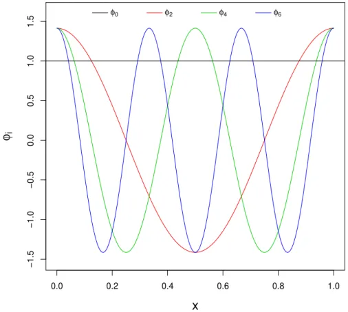
Note that there are also many possible smoothness and/or boundary conditions (like twice differentiability) to ensure a somewhat fast convergence rate (seeEfromovich(1999) for details). Intuitively, the less smooth the function f is, the larger will be the number of necessary components to get a reasonable approximation. To give the reader some intuition on this, Figure 1shows the curves for some of the components of Fourier series. It can be seen that higher order
components are needed in order to better “explain” less smooth functions.
We now proceed with the exposition of the procedures for statistical inference using frequentist and Bayesian approaches in sections2.1and2.2, respectively.
2.1
Frequentist Inference
Given i.i.d. random variablesY1,Y2, ...,Ynwith density function f :[0,1]→R∈L2[0,1],
a simple approach to infer f from a frequentist perspective using Fourier series is to use:
ˆ
fI(y) =1+ I
∑
i=1
b
αiφi(y)
where
b
αi= 1 n
n
∑
j=1
φi(Yj)≈ Z
2.1. Frequentist Inference 27
0.0 0.2 0.4 0.6 0.8 1.0
−1.5 −1.0 −0.5 0.0 0.5 1.0 1.5 x φi
φ0 φ2 φ4 φ6
Figure 1 – Plot of some of the components of Fourier series: if a linear combination of such functions is used to approximate a function f, then it can be easily seen that the less smooth f is, the larger will be number of Fourier series components needed in order to better “explain” f.
This estimator is a special case of the modulator estimator which can found inWasserman (2006), where we can also find the expected value and variance of eachαbi:
E(αbi) = Z 1
0 φi(x)f(x)dx=θi
Var(αbi) = R1
0 φi2(x)f(x)dx−θi2 n
as well as risk of the estimator ˆfI:
R(fˆI;f) =E Z 1
0 (
ˆ
fI(x)−f(x))2dx
=
I
∑
i=1
Var(αbi) +
∞
∑
i=I+1
θi2
Therefore the choice of the estimator cutoff parameterI can be seen as bias-variance trade-off problem (in practice, a possible solution is to use cross-validation to chooseI).
28 Chapter 2. Nonparametric density estimation via Fourier series
2.2
Bayesian Inference
Just as in the previous section, given i.i.d. random variablesY1,Y2, ...,Ynwith density function f :[0,1]→R∈L2[0,1], directly proceeding with the Bayesian inference (which is the
focus of this work) of f using Fourier series is a somewhat difficult problem since we have to define and work with priors in the constrained space where f(y)≥0 for ally∈[0,1].
One way to overcome this issue is to use the approach of sieve priors suggested by Scricciolo(2006), which places a prior directly on the coefficient vectorβ of the Fourier series expansion of log(f) (instead of f) so that conditionally on the threshold parameter (cutoff parameter)Iwe have:
f(y|I,β) = 1
g(β,I)exp
( I
∑
i=1
βiφi(y) )
wheregis a normalizing factor such that
g(β,I) =
Z 1
0 exp
( I
∑
i=1
βiφi(y) )
dy
which is necessary in order to haveR01f(y|I,β)dy=1. Note that eachβilives inR, which solves the constrained space problem.
As a drawback, we introduced the difficulty of calculating a normalizing factor (using numerical integration) when evaluating the likelihood function1.
With such approach (ofScricciolo(2006)) we have
βi∼Normal(0,(i+1)−2p−1) ifi∈ {1,3,5, ...}
βi∼Normal(0,i−2p−1) ifi∈ {2,4,6, ...}
as prior distributions (with eachβiindependent from each other) for the Fourier series coefficients, where p is a strictly positive natural number and the normal distribution is parameterized in terms of mean and variance.
The approach also places a prior distribution on the threshold parameterI, such that for allkstrictly positive natural number:
P(I=k) = exp{−γk}
∑∞i=1exp{−γi}
(a geometric distribution) which therefore gives us a Bayesian mixture of Fourier series models. Hereγ a is positive hyperparameter.
As we saw in the beginning of this chapter, the less smooth the function is, the greater will number of components needed to get an arbitrary good approximation. Therefore the intuition 1 This was addressed by adding a numerical integrator toStan, which by time of submission of this
2.2. Bayesian Inference 29
behindP(I=k)decreasing onkis that we are assuming a prior belief on a somewhat smooth structure for thePDF(seeScricciolo(2006)). This also justifies the use of decreasing variances in priors forβi(asi→∞). In principle, one could wonder whether it would be better to not assume this smooth structure and work with more general prior assumptions, but as we saw in section 2.1, we would incur in a problem of lower bias, but greater variance which in general would lead to estimates of f that overfits data.
In this work, primarily because of computational and time restrictions we worked with the series with I up to 10 (that is,P(I=k) =0 ifk>10)2. We choose to work with somewhat conservative values for those priors withp=1 andγ =1/10. As we will see in the next chapters, the results were reasonable for the chosen prior distributions.
2 There are two technical justifications for this not being problematic: firstP(I=k)quickly decreases to
zero (a priori) ask→∞, and also the prior distribution forβiquickly concentrates on zero (since its
31
CHAPTER
3
HMC, NUTS AND STAN
To obtain the posterior samples of the Fourier series models studied in this work, we usedStan(Stan Development Team,2014), which is a statistical software for obtaining Markov Chain Monte Carlo (MCMC) samples1using either the algorithm Halmiltonian Monte Carlo (HMC)2or the algorithm No-U-Turn Sampler (NUTS).
TheHMCis a MCMC sampling algorithm that was brought from Hamiltonian molecular dynamics to statistics byDuaneet al.(1987) andNeal(2011). The idea is to solve an
Hamil-tonian dynamic simulation problem where the variables of original problem (sampling from a target distribution) will be the position variables of Halmitonian system and new artificially introduced variables, typically with Gaussian distribution, will be the “momentum variables” of the Halmitonian system (NEAL,2011). Among other advantages, theHMCutilizes the gradient of the log-posterior to produce less correlated samples.
The sampler requires, in practice, at least two sampler specific parameters called number of leapfrogs steps and leapfrog stepsize: what happens is that if one could solve the HMC dif-ferential equations exactly, it would be possible to sample using only a single sampler specific parameter: the “size”, that is, the size of the “jump” we do on the differential equation system for each new sample we want.
However, except for very simple toy models, this is not possible and the differential equation system needs to be approximated using the leapfrog method: approximate the full differential equation jump by many little steps on a difference equations system (similar to Euler method). In any case,HMCis very sensible to these parameters and manually tuning them requires some expertise.
NUTSis a variation of theHMCdescribed atHoffman and Gelman(2014) that doesn’t
1 Stancan also be used to do optimization and variational inference.
2 It was originally called Hybrid Monte Carlo byDuaneet al.(1987), but the term Hamiltonian Monte
32 Chapter 3. HMC, NUTS and Stan
require the user to set one the sampler specific parameter: the number of leapfrogs steps. Instead of having an specific number of leapfrog steps, the algorithm will advance in the trajectory up to the point where it starts to retraces its steps (hence the name No-U-Turn Sampler). The authors of the algorithm also propose a method for adapting the other sampler specific parameter left (leapfrog stepsize).
Either way, implementation of any of the algorithms requires time and some expertise and one also needs to code the log-posterior function and its gradient for each model. The process is clearly time-consuming and error-prone, but it’s done automatically byStanonce the user specify the model inStanlanguage which will handle internally theHoffman and Gelman (2014) algorithm without requiring any configuration by the user.
3.1
Stan and discrete parameters
Stancannot sample models with discrete parameters directly: this is due to the inability ofHMC/NUTSto sample discrete variables since they are not differentiable.
However this can be accomplished by marginalizing out the discrete parameters. Suppose, for instance, thatH∈His a discrete parameter andθ ∈Θis the vector of all the other (continuous) parameters. Then we can get the (marginal) likelihood ofθ by averaging over all possible values ofH,
P(Y|θ) =
∑
h∈H
P(Y|θ,H=h)P(H=h|θ) (3.1)
whereY is the vector containing all known data. After obtainingSsimulations (a1,a2, ...,aS) from posteriorP(θ|Y)of the “marginalized model”, one can proceed directly to get, for example, the posterior predictive distribution of some ˜Y,
P(Y˜|Y) =
Z
Θh
∑
∈HP(˜
Y,θ,H=h|Y)dθ
=
Z
Θh
∑
∈HP(Y˜|θ,H=h,Y)P(H=h|θ,Y)P(θ|Y)dθ
≈ 1S
S
∑
j=1h
∑
∈HP(Y˜|θ =aj,H =h,Y)P(H=h|θ =aj,Y)
Note that
P(H=h|θ =aj,Y) =
P(Y|θ =aj,H=h)P(H=h|θ =aj)
∑k∈HP(Y|θ =aj,H=k)P(H =k|θ =aj)
(3.2)
which are terms that we already calculated (in equation3.1) for each posterior simulation. It is easy to get the posterior forH averaging over the probability in equation3.2,
P(H=h|Y)≈1
S S
∑
j=1
3.1. Stan and discrete parameters 33
We can also use it to get the (conditional) posterior forθ|H,
P(θ ∈B|H=h,Y)
= PR(H=h|θ ∈B,Y)P(θ ∈B|Y)
ΘP(H=h|θ,Y)P(θ|Y)dθ
≈1S
S
∑
j=1
IB(aj)P(H=h|θ =aj,Y)
P(H=h|θ =aj,Y)
whereIis the indicator function. That is, for eachh∈Hwe haveSweighted posterior simulations
whereθ=aj|H=hhas relative weightP(H=h|θ=aj,Y). SeeStan Development Team(2014) for more details.
The main weakness of this method of marginalization of discrete parameters is that we have to calculate P(Y,H =h|θ) for every h∈H every time we want the likelihoodP(Y|θ),
making it computationally unfeasible whenHis huge (unless the model has a known shortcut to
calculate the sum in equation3.1). However, this method has an advantage over methods like Metropolis and Gibbs that explore only a single “marginalized model” (sampleθ givenH) for each simulation: those methods might explore well only some of the models (those with high posterior probability), and might actually get stuck in a single “marginalized model”, not being ergodic.
Imagine for instance that,H∈ {h1,h2}, and that the region for continuous parameterθ
whereP(θ|H=h1)>0 is disjoint from the region whereP(θ|H=h2)>0. Then, if we a start a
Gibbs sampler at sayH=h1, it will get stuck on it forever sinceP(H=H2|θ)/P(H=H1|θ)will
always evaluate to zero and if we are using Metropolis and the proposal samples the parameters in block, we might still get stuck if the regions are very close from each other and the proposal has difficulty “connecting” each of them (this is specially troublesome for high dimensionalθ). This is a extreme case, but something less extreme may also be very detrimental, the regions might not be disjoint, but the union might be a set with very little probability (again, this gets worse with high dimensionality) to the point where they are "probabilistic" disjoint with our finite computational resources.
35
CHAPTER
4
A SIMULATION STUDY TO ASSESS THE
PERFORMANCE OF THE METHOD
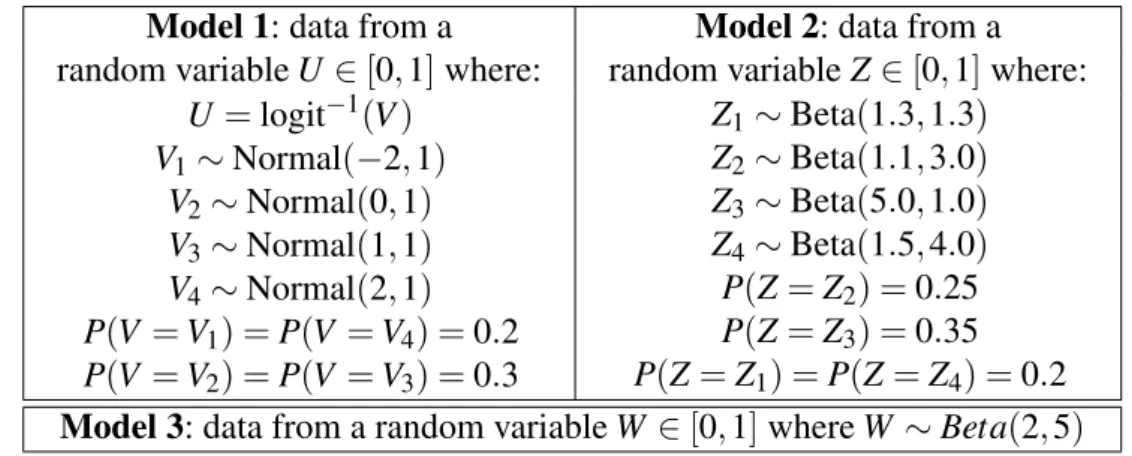
In this chapter we present the results of a simulation study performed to assess the performance of the Fourier series method compared to the kernel density estimation (KDE). We worked with datasets being generated 100 times from 3 different true models with each dataset having 50 observations. We describe those 3 data generating models in Table1.
Table 1 – Description of the models used to generate data for the simulation study in this chapter and the next one.
Model 1: data from a Model 2: data from a random variableU ∈[0,1]where: random variableZ∈[0,1]where:
U =logit−1(V)
V1∼Normal(−2,1)
V2∼Normal(0,1)
V3∼Normal(1,1)
V4∼Normal(2,1)
P(V =V1) =P(V =V4) =0.2
P(V =V2) =P(V =V3) =0.3
Z1∼Beta(1.3,1.3)
Z2∼Beta(1.1,3.0)
Z3∼Beta(5.0,1.0)
Z4∼Beta(1.5,4.0)
P(Z=Z2) =0.25
P(Z=Z3) =0.35
P(Z=Z1) =P(Z=Z4) =0.2
Model 3: data from a random variableW ∈[0,1]whereW ∼Beta(2,5)
Using data from these true models, we fitted Fourier Series models conditional on I =1,2, ...,10 and the Bayesian mixture of those 10 models (sieve prior onI, as explained in chapter2). For comparison purposes, we also fitted the same data usingKDEmethod ofSheather (1991).
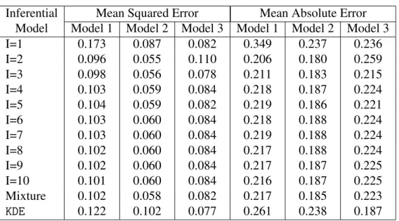
In Table2, we presented the estimates of the errors for each true model from Table1, using the following procedure fori∈ {1,2,3}:
36 Chapter 4. A simulation study to assess the performance of the method
2. Fit data using Fourier series (calculateE[f|D]) andKDE(calculate ˆf).
3. Calculate the integrated squared error for Fourier series (R01(f(y)−E[f(y)|D])2dy) and forKDE(R1
0(f(y)−fˆ(y))2dy).
4. Calculate the integrated absolute error for Fourier series (R01|f(y)−E[f(y)|D]|dy) and for KDE(R1
0
f(y)− fˆ(y)dy).
5. Repeat the procedure 100 times and average over the results.
Hence, the table presents the estimates of expected integrated mean squared error (MSE) Z
D Z 1
0 (f(y)−E[f(y)|D]) 2dy P(
D|f)dD
=ED Z 1
0 (f(y)−E[f(y)|D])
2dy
and the expected integrated mean absolute error (MAE)
ED Z 1
0 |f(y)−E[f(y)|D]|dy
for each true model f(y).
Table 2 – Estimated mean squared error and mean absolute error for 3 different data generating models (true models, see Table1) which were used to fit a Fourier series model with up to 10 component functions and a mixture model of those 10 models (a sieve prior). For comparison purposes, data were also used in aKDEmethod.
Inferential Mean Squared Error Mean Absolute Error Model Model 1 Model 2 Model 3 Model 1 Model 2 Model 3
I=1 0.173 0.087 0.082 0.349 0.237 0.236
I=2 0.096 0.055 0.110 0.206 0.180 0.259
I=3 0.098 0.056 0.078 0.211 0.183 0.215
I=4 0.103 0.059 0.084 0.218 0.187 0.224
I=5 0.104 0.059 0.082 0.219 0.186 0.221
I=6 0.103 0.060 0.084 0.218 0.188 0.224
I=7 0.103 0.060 0.084 0.219 0.188 0.224
I=8 0.102 0.060 0.084 0.217 0.188 0.224
I=9 0.102 0.060 0.084 0.217 0.187 0.225
I=10 0.101 0.060 0.084 0.216 0.187 0.225
Mixture 0.102 0.058 0.082 0.217 0.185 0.223
KDE 0.122 0.102 0.077 0.261 0.238 0.187
The Bayesian mixture of Fourier series models with sieve prior (and even most of its component models individually) have outperformed theKDEfor true models 1 and 2, but haven’t done so for true models 3.
37
0.0 0.2 0.4 0.6 0.8 1.0
0.6
1.0
1.4
1.8
Estimated density for I=1
y
Density
0.0 0.2 0.4 0.6 0.8 1.0
0.6
1.0
1.4
1.8
Estimated density for I=2
y
Density
0.0 0.2 0.4 0.6 0.8 1.0
0.6
1.0
1.4
1.8
Estimated density for I=3
y
Density
0.0 0.2 0.4 0.6 0.8 1.0
0.6
1.0
1.4
1.8
Estimated density for I=5
y
Density
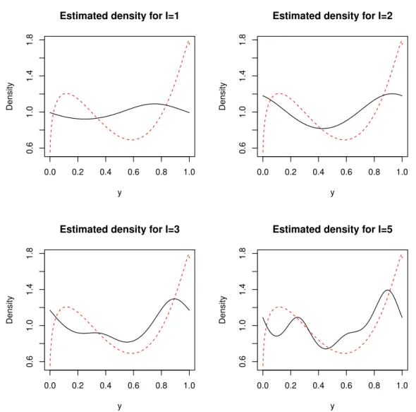
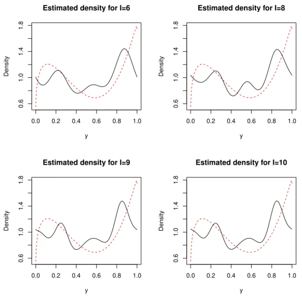
Figure 2 – Plots of the average estimated density using Fourier series for low values ofI, data came from (a single dataset of) true model 2. For comparison, the true density is also shown (as a dotted red line).
I=7 for reasons of brevity) using data from a single dataset from true model 2. For comparison, the true density is also shown (as a dotted red line).
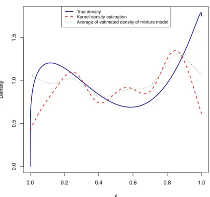
Figure5shows plots of the curves of the average estimated density from the Bayesian mixture Fourier series model and of the estimate fromKDEusing the same data (a single dataset from true model 2). Figures 4and6do the same for true models 1 and 3, also using a single dataset from these true models.
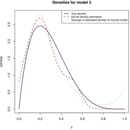
These 3 Figures suggest that the Bayesian Fourier series mixture model have performed reasonably well over the whole the domain[0,1]of the density function, but they explored only a single dataset generated from each true model. On the other hand, Table2gave us the average errors using 100 different datasets from the true models, but the errors were integrated over[0,1].
38 Chapter 4. A simulation study to assess the performance of the method
0.0 0.2 0.4 0.6 0.8 1.0
0.6
1.0
1.4
1.8
Estimated density for I=6
y
Density
0.0 0.2 0.4 0.6 0.8 1.0
0.6
1.0
1.4
1.8
Estimated density for I=8
y
Density
0.0 0.2 0.4 0.6 0.8 1.0
0.6
1.0
1.4
1.8
Estimated density for I=9
y
Density
0.0 0.2 0.4 0.6 0.8 1.0
0.6
1.0
1.4
1.8
Estimated density for I=10
y
Density
Figure 3 – Plots of the average estimated density using Fourier series for high values ofI, data came from (a single dataset of) true model 2. For comparison, the true density is also shown (as a dotted red line).
over[0,1]).
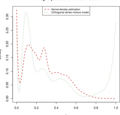
Therefore, Figures7,8and9show a plot of the estimatedMSEof the Bayesian mixture Fourier series model and KDEmodels for each point in [0,1]for the true models 1, 2 and 3 (respectively) using those 100 different datasets. That is, we estimated and plotted the value of
ED(f(y)−E[f(y)|D])2
for a grid of valuesy∈[0,1]. Therefore, if those plotted curves are integrated against yover
[0,1], we’ll get the squared errors shown in Table2.
39
0.0 0.2 0.4 0.6 0.8 1.0
0.0
0.5
1.0
1.5
2.0
Densities for model 1
y
Density
True density
Kernel density estimation
Average of estimated density of mixture model
Figure 4 – Average estimated density from the Bayesian mixture of the 10 Fourier series models (sieve prior) against the estimate fromKDE, data came from true model 1 (see Table1) which is also
plotted.
40 Chapter 4. A simulation study to assess the performance of the method
0.0 0.2 0.4 0.6 0.8 1.0
0.0
0.5
1.0
1.5
Densities for model 2
y
Density
True density
Kernel density estimation
Average of estimated density of mixture model
Figure 5 – Average estimated density from the Bayesian mixture of the 10 Fourier series models (sieve prior) against the estimate fromKDE, data came from true model 2 (see Table1) which is also
41
0.0 0.2 0.4 0.6 0.8 1.0
0.0
0.5
1.0
1.5
2.0
2.5
Densities for model 3
y
Density
True density
Kernel density estimation
Average of estimated density of mixture model
Figure 6 – Average estimated density from the Bayesian mixture of the 10 Fourier series models (sieve prior) against the estimate fromKDE, data came from true model 3 (see Table1) which is also
plotted.
0.0 0.2 0.4 0.6 0.8 1.0
0.0
0.5
1.0
1.5
2.0
Average squared error for true model 1
y
Density
Kernel density estimation Orthogonal series mixture model
42 Chapter 4. A simulation study to assess the performance of the method
0.0 0.2 0.4 0.6 0.8 1.0
0.0
0.2
0.4
0.6
0.8
1.0
Average squared error for true model 2
y
Density
Kernel density estimation Orthogonal series mixture model
Figure 8 – Estimated mean squared error using data from true model 2 (see Table1). Data was used to fit a Bayesian mixture of Fourier series model and, for comparison purposes, aKDEmodel.
0.0 0.2 0.4 0.6 0.8 1.0
0.00
0.05
0.10
0.15
0.20
0.25
0.30
Average squared error for true model 3
y
Density
Kernel density estimation Orthogonal series mixture model
43
CHAPTER
5
TWO-SAMPLE SIMILARITY ANALYSIS
In this chapter we deal with the question of how to measure the uncertainty regarding the distance between two populations1. That is, given two samplesD
1andD2from two (possibly
different) populations withPDFs f1and f2, how close (do we expect) the distributions of those two populations are to each other?
To solve this problem we evaluate the posterior probability of some measure of distance (metric), here we work with the integrated squared distance which we denote byM:
M(f1,f2) =
Z 1
0 (f1(y)− f2(y)) 2dy
This distance is itself a parameter, and therefore it has a posterior probability distribution
M(f1,f2)|D1,D2. Having the posterior probability of this distance, we can proceed to calcute
P(M(f1,f2)<ε|D1,D2)which gives us a probability that the two populations are close to each
other (in the integrated squared distance “sense”) up to an arbitrary pointε.
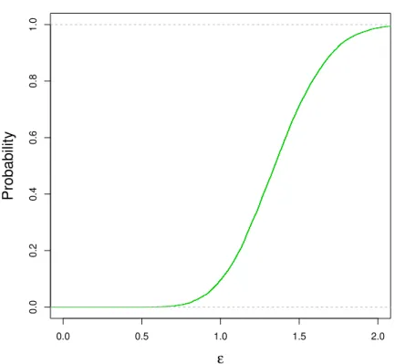
To give the reader some intuition regarding the relationship ofP(M(f1,f2)<ε|D1,D2)
andε, in Figure10we show a plot of the value ofP(M(f1,f2)<ε|D1,D2)against the value of
ε withD1andD2being datasets generated from true model 1 (see Table1). The Figure indicates
that there is a high probability that the distributions are close to each other; compare to Figure11 whereD1is generated from true model 1, butD2is generated from true model 3.
In this chapter, with the purpose of performing some simulation studies, we work from now on with a fixed value forε which we’ll callε0:
ε0=
Z +∞
−∞ (ϕ0(y)−ϕ1(y))
2dy
≈0.125
Hereϕ0is thePDFof a standard Gaussian distribution andϕ1is thePDFof a Gaussian
distribution with mean 1 and standard deviation 1.
44 Chapter 5. Two-sample similarity analysis
0.0 0.5 1.0 1.5 2.0
0.0
0.2
0.4
0.6
0.8
1.0
ε
Probability
Figure 10 – Plot ofP(M(f1,f2)<ε|D1,D2)againstε. Here bothD1andD2are datasets generated from
true model 1 (see Table1).
0.0 0.5 1.0 1.5 2.0
0.0
0.2
0.4
0.6
0.8
1.0
ε
Probability
Figure 11 – Plot ofP(M(f1,f2)<ε|D1,D2)againstε. HereD1is a dataset generated from true model 1
5.1. Simulation study for samples from the same population 45
After having the theoretic aspects been settled down, we now proceed to some simulation studies with the intention of evaluating the performance of our approach.
5.1
Simulation study for samples from the same
popula-tion
We start with a simulation study with samples from the same population given the following procedure:
1. Generate 2 samplesD1andD2from true modeli.
2. Fit the Fourier series model using each sample separately (get MCMC simulations of f1|D1and f2|D2).
3. Using the simulations from step 2, generate simulations forM(f1,f2)|D1,D2.
4. Get the proportion of simulations that are belowε0, therefore obtaining approximately
P(M(f1,f2)<ε0|D1,D2)
5. Repeat the procedure 50 times.
The results for such procedure are shown in Figures12,13and 14for true models 1, 2 and 3 respectively where each of the 50 repetions of the procedure are plotted (points were sorted before being plotted). An horizontal green line in Figures which is the mean of all points and therefore is an approximation to
Z
D Z
D
P(M(f1,f2)<ε0|D1,D2)P(D1|f1)dD1P(D2|f2)dD2
Since the “true distanceM” from a true model to itself is 0, we should be able to observe
a reasonable probability for the event(M(f1,f2)<ε0|D1,D2), and indeed this is the case for
46 Chapter 5. Two-sample similarity analysis ● ● ● ● ●● ● ● ● ● ● ● ● ● ● ● ● ● ●● ● ●● ●● ●● ● ●● ● ● ● ● ●● ● ● ●● ● ● ●● ● ● ● ● ● ●
0 10 20 30 40 50
0.0
0.2
0.4
0.6
0.8
Generated sample (index)
Probability
Figure 12 – Each plotted point is the estimated probability that the integrated squared distance between the
PDFs of the two samples is less thanε0(that is,P(R1
0(f1(y)−f2(y))2dy<ε0|D1,D2)) given
samplesD1andD2(for each plotted point, 2 different dataset were generated)both generated from true model 1(see Table1). Points were sorted before plotting. We’ve choosen to use, as the value ofε0, the integrated squared distance between thePDFof a standard Gaussian and
thePDFof a Gaussian with mean 1 and standard deviation 1 as the value ofε0. The horizontal
green line is the mean of all points.
● ● ●● ●● ● ● ● ● ●● ● ●● ● ● ●● ● ● ● ● ●● ● ● ● ● ● ● ● ●● ● ● ● ● ●● ● ● ● ●● ● ● ● ● ●
0 10 20 30 40 50
0.2
0.4
0.6
0.8
Generated sample (index)
Probability
Figure 13 – Each plotted point is the estimated probability that the integrated squared distance between the
PDFs of the two samples is less thanε0(that is,P(R1
0(f1(y)−f2(y))2dy<ε0|D1,D2)) given
samplesD1andD2(for each plotted point, 2 different dataset were generated)both generated from true model 2(see Table1). Points were sorted before plotting. We’ve choosen to use, as the value ofε0, the integrated squared distance between thePDFof a standard Gaussian and
thePDFof a Gaussian with mean 1 and standard deviation 1 as the value ofε0. The horizontal
5.2. Simulation study for samples from the different populations 47 ● ●● ● ● ● ● ●● ● ●● ● ● ●● ● ● ● ● ●● ● ● ● ● ●● ● ● ● ●● ●● ● ● ●● ●● ● ● ●● ●● ● ● ●
0 10 20 30 40 50
0.0
0.2
0.4
0.6
0.8
Generated sample (index)
Probability
Figure 14 – Each plotted point is the estimated probability that the integrated squared distance between the
PDFs of the two samples is less thanε0(that is,P(R1
0(f1(y)−f2(y))2dy<ε0|D1,D2)) given
samplesD1andD2(for each plotted point, 2 different dataset were generated)both generated from true model 3(see Table1). Points were sorted before plotting. We’ve choosen to use, as the value ofε0, the integrated squared distance between thePDFof a standard Gaussian and
thePDFof a Gaussian with mean 1 and standard deviation 1 as the value ofε0. The horizontal
green line is the mean of all points.
5.2
Simulation study for samples from the different
pop-ulations
In this section we have a similar procedure, but with samplesD1andD2coming from
different true models:
1. Generate sampleD1from true modeliand sampleD2from true model j.
2. Fit the Fourier series model using each sample separately (get MCMC simulations of f1|D1and f2|D2).
3. Using the simulations from step 2, generate simulations forM(f1,f2)|D1,D2.
4. Get the proportion of simulations that are belowε0, thefore obtaining approximately
P(M(f1,f2)<ε0|D1,D2)
5. Repeat the procedure 100 times.
48 Chapter 5. Two-sample similarity analysis ●●●●● ● ●●● ●●●●●● ●●●● ● ●●●● ●●●●● ●● ●●●●●●● ●●● ● ●● ●●● ●●● ●●●● ●● ●●●● ●●● ●●●● ●●● ●●●● ●● ●●●●● ●●●●● ●● ●● ●●● ●●● ● ● ●●
0 20 40 60 80 100
0.0
0.2
0.4
0.6
0.8
Generated sample (index)
Probability
Figure 15 – Each plotted point is the estimated probability that the integrated squared distance between the PDFs of the two samples is less thanε0 (that is, P(R1
0(f1(y)−f2(y))2dy<ε0|D1,D2))
given samplesD1andD2(for each plotted point, 2 different dataset were generated) whereD1 was generated from true model 1, andD2was generated from true model 2(see Table
1). Points were sorted before plotting. We’ve choosen to use, as the value ofε0, the integrated
squared distance between thePDFof a standard Gaussian and thePDFof a Gaussian with
mean 1 and standard deviation 1. The horizontal green line is the mean of all points.
manner, each of the 100 repetitions of the procedure are plotted (points were sorted before being plotted). We used the same value forε0and the plots also include an horizontal green line in plot
which is the mean of all points.
Note that the “true distanceM”:
∙ Between true model 1 and true model 2 is approximately 0.118.
∙ Between true model 1 and true model 3 is approximately 1.280.
∙ Between true model 2 and true model 3 is approximately 0.881.
and, as we have already seen, ε0≈0.125, so it does make sense that, as we can see
on Figure15, samples from true model 1 and 2 have a reasonable probability for the event
(M(f1,f2)<ε0|D1,D2). On the other hand, this probability should be low if samples come from
true model 1 and 3, or from true models 2 and 3, and this is what one can clearly see on Figures 16and17.
5.3. An example of two-sample similarity analysis with real data 49
●●●●●●●●●●●●●●●●●●●●●●●●●●●●●●●●●●●●●●●●●●●●●●●●●●●●●●●●●●●●●●●●●●●●●●●●●●●●●●●●●●●●●●●●●●●●●●●●● ●●
●
0 20 40 60 80 100
0e+00 1e−04 2e−04 3e−04 4e−04 5e−04 6e−04
Generated sample (index)
Probability
Figure 16 – Each plotted point is the estimated probability that the integrated squared distance between the PDFs of the two samples is less thanε0 (that is, P(R1
0(f1(y)−f2(y))2dy<ε0|D1,D2))
given samplesD1andD2(for each plotted point, 2 different dataset were generated) whereD1 was generated from true model 1, andD2was generated from true model 3(see Table
1). Points were sorted before plotting. We’ve choosen to use, as the value ofε0, the integrated
squared distance between thePDFof a standard Gaussian and thePDFof a Gaussian with
mean 1 and standard deviation 1. The horizontal green line is the mean of all points.
5.3
An example of two-sample similarity analysis with
real data
We now present an example of two-sample similarity analysis using real data. We used data from the Montreal cognitive assessment used inCecatoet al.(2016).
Here we have 3 groups patients:DArepresents the group of patients diagnosed with Alzheimer,CCLrepresents the group of patients diagnosed with a light cognitive decay and GCrepresents the control group (the response measures the performance of each patient on the Montreal cognitive assessment).
Data was transformed to[0,1]usingS= (R−50)/(107−50). Although the maximum values and minimum possible values for this test are 0 and 107, we decided a priori, specially for simplicity, to assume the minimum value to be 50, since it would be very unlikely to a person with such a score to even be placed to take such test.
For simplicity, we have also eliminated two missing data points from datasets. After transformation and removal of missing data, we had 45, 52 and 39 observations forCCL,DA andGCgroups, respectively and the descriptive statistics presented in Table3.
50 Chapter 5. Two-sample similarity analysis ●●●●●●●●●●●●●●●●●●●●●●●●●●●●●●●●●●●●●●●●●●●●●●●●●●●●●●●●●●●●●●●●●●●●●●●●●●●●●●●●●●●●●●●●●●● ●●● ● ●●● ● ●
0 20 40 60 80 100
0.00
0.05
0.10
0.15
0.20
Generated sample (index)
Probability
Figure 17 – Each plotted point is the estimated probability that the integrated squared distance between the PDFs of the two samples is less thanε0 (that is, P(R1
0(f1(y)−f2(y))2dy<ε0|D1,D2))
given samplesD1andD2(for each plotted point, 2 different dataset were generated) whereD1 was generated from true model 2, andD2was generated from true model 3(see Table
1). Points were sorted before plotting. We’ve choosen to use, as the value ofε0, the integrated
squared distance between thePDFof a standard Gaussian and thePDFof a Gaussian with
mean 1 and standard deviation 1. The horizontal green line is the mean of all points.
Table 3 – Descriptive statistics of data used in this section.
Obs Min 1st Qu Median Mean 3rd Qu Max SD CCL 45 0.4035 0.6140 0.6842 0.6737 0.7719 0.8772 0.1163
DA 52 0.0351 0.3421 0.5263 0.4716 0.6272 0.8070 0.2042 GC 39 0.5614 0.7632 0.8596 0.8376 0.9123 1.0000 0.0941
average estimated densities of each group using the Fourier series method. Figure19shows a plot ofP(M(f1,f2)<ε|D1,D2)againstεcomparing each of groups against each other (therefore,
totaling 3 comparisons).
5.3. An example of two-sample similarity analysis with real data 51
0.0 0.2 0.4 0.6 0.8 1.0
0.0
0.5
1.0
1.5
2.0
2.5
3.0
3.5
Estimated densities
s
Density
CCL DA GC
Figure 18 – Plots of the average estimated density using Fourier series (using real data). Here we have 3 groups patients: DArepresents the group of patients diagnosed with Alzheimer, CCL
52 Chapter 5. Two-sample similarity analysis
0 1 2 3 4
0.0
0.2
0.4
0.6
0.8
1.0
ε
Probability
CCL against DA CCL against GC DA against GC
Figure 19 – Plot ofP(M(f1,f2)<ε|D1,D2)againstε (using real data). Here bothD1andD2are datasets
for the observations groupsCCL,DAandGC(being compared against each other). Here we have 3 groups patients:DArepresents the group of patients diagnosed with Alzheimer,CCL
53
CHAPTER
6
CONCLUSION
In this work, we proposed a comparison study between Bayesian Fourier series and the kernel density estimation. We concluded that Fourier series method has reasonable goodness of fit compared to the kernel density estimation method and that both often had problems to estimate thePDFnear the boundaries for reasonable samples sizes.
We also proposed a method to verify the ability of the Fourier series method to measure the uncertainty regarding the similarity between two populations. We conclude that the proposed method is reasonable for such objective. In particular, it yielded sensible results in a real application. We notice that other Bayesian density estimators could be used; our framework for comparing two populations is very general with that respect.
Possible extensions of this work are:
∙ A rerun the simulation studies using different true models and/or different samples sizes.
∙ Usage of other orthogonal series other than Fourier series.
∙ A comparison of the proposed Bayesian density estimation method with other established methods other thanKDE.
∙ Use different sieve prior parameters, possibly using cross validation to choose them.
∙ A case study (using real data) of the two sample comparison method.
∙ Proposal of a method to obtainε, possibly justifying that using a loss function and Decision Theory techniques.
55
BIBLIOGRAPHY
CECATO, J. F.; MARTINELLI, J. E.; IZBICKI, R.; YASSUDA, M. S.; APRAHAMIAN, I. A subtest analysis of the montreal cognitive assessment (moca): which subtests can best discriminate between healthy controls, mild cognitive impairment and alzheimer’s disease? International Psychogeriatrics, Cambridge University Press, Cambridge, UK, v. 28, n. 5, p. 825–832, 005 2016. Citation on page49.
DUANE, S.; KENNEDY, A.; PENDLETON, B. J.; ROWETH, D. Hybrid monte carlo.Physics Letters B, v. 195, n. 2, p. 216 – 222, 1987. ISSN 0370-2693. Citation on page31.
EFROMOVICH, S. Nonparametric curve estimation: methods, theory and applications. New York: Springer, 1999. ISBN 0-387-98740-1. Citation on page26.
GELMAN, A.; CARLIN, J. B.; STERN, H. S.; DUNSON, D. B.; VEHTARI, A.; RUBIN, D. B. Bayesian data analysis. Third. [S.l.]: CRC Press, 2014. ISBN 978-143984095-5. Citation on page23.
GLAD, I. K.; HJORT, N. L.; USHAKOV, N. G. Correction of density estimators that are not densities.Scand J Stat, Wiley-Blackwell, v. 30, n. 2, p. 415–427, jun 2003. Citation on page 27.
HOFFMAN, M. D.; GELMAN, A. The No-U-Turn Sampler: Adaptively setting path lengths in Hamiltonian Monte Carlo.Journal of Machine Learning Research, v. 15, p. 1593–1623, 2014. Citations on pages31e32.
HOLMES, C. C.; CARON, F.; GRIFFIN, J. E.; STEPHENS, D. A. Two-sample Bayesian nonparametric hypothesis testing.Bayesian Anal., International Society for Bayesian Analysis, v. 10, n. 2, p. 297–320, 06 2015. Citation on page23.
KREYSZIG, E. Introductory Functional Analysis with Applications. [S.l.]: Wiley, 1989. ISBN 0471504599. Citation on page26.
LAVINE, M. Some aspects of polya tree distributions for statistical modelling. Ann. Statist., The Institute of Mathematical Statistics, v. 20, n. 3, p. 1222–1235, 09 1992. Citation on page23.
MÜLLER, P.; VIDAKOVIC, B. Bayesian inference with wavelets: Density estimation.Journal of Computational and Graphical Statistics, Taylor & Francis Group, v. 7, n. 4, p. 456–468, 1998. Citation on page23.
NEAL, R. M. Mcmc using hamiltonian dynamics. In: BROOKS ANDREW GELMAN, G. L. J. S.; MENG, X.-L. (Ed.).Handbook of Markov chain Monte Carlo. Boca Raton, USA: CRC PressTaylor & Francis, 2011. ISBN 1420079417. Citation on page31.
56 Bibliography
PETRONE, S.; WASSERMAN, L. Consistency of bernstein polynomial posteriors.Journal of the Royal Statistical Society: Series B (Statistical Methodology), Wiley Online Library, v. 64, n. 1, p. 79–100, 2002. Citation on page23.
RIVOIRARD, V.; ROUSSEAU, J.et al.Posterior concentration rates for infinite dimensional exponential families.Bayesian Analysis, International Society for Bayesian Analysis, v. 7, n. 2, p. 311–334, 2012. Citation on page23.
SCRICCIOLO, C. Convergence rates for Bayesian density estimation of infinite-dimensional exponential families.The Annals of Statistics, v. 34, n. 6, p. 2897–2920, 2006. Citations on pages11,13,23,24,28e29.
SHEATHER, M. C. J. S. J. A reliable data-based bandwidth selection method for kernel den-sity estimation.Journal of the Royal Statistical Society. Series B (Methodological), [Royal Statistical Society, Wiley], v. 53, n. 3, p. 683–690, 1991. ISSN 00359246. Citation on page35. SORIANO, J.Bayesian Methods for Two-Sample Comparison. Phd Thesis (PhD Thesis) — Duke University, 2015. Citation on page23.
Stan Development Team. Stan Modeling Language Users Guide and Reference Manual, Version 2.8.0. [S.l.], 2014. Citations on pages31e33.