RETAIL IN THE EMERGING MARKETS: A STUDY
BASED ON ASSOCIATION RULES
Joaquim Alexandre de Freitas Justino
2
NOVA Information Management School
Instituto Superior de Estatística e Gestão de Informação
Universidade Nova de Lisboa
RETAIL IN THE EMERGING MARKETS: A STUDY BASED ON
ASSOCIATION RULES
by
Joaquim Alexandre de Freitas Justino
Dissertation for obtaining the Master’s degree in Information Management, with a specialization in Knowledge Management and Business Intelligence
Advisor:Fernando Bação
Co Advisor: Vasco Jesus
3 ABSTRACT
Buying patterns and habits of consumers in the developed countries are fairly well known. There is plenty of information, ranging from market data collected by companies like Nielsen, to data collected at the Point-Of-Sale (POS) by retailers. This data provides a detailed image of the buying habits of consumers in developed countries. In emerging countries however, our knowledge of the habits and behaviors is limited since this kind of data is scarce. With the expansion of modern retail companies to emerging countries, and their data collecting technologies, new opportunities emerge to understand these customers. This work is interested in contrasting habits and behaviors of customers in developed and emerging countries. The project seeks to understand the main differences between these consumers through the exploration of POS data using Association Rules. POS data and Association Rules provide a very rich and powerful way to understand the main traits of commerce and consumers. The ability to explore very big databases and extract significant facts and regularities in day-to-day transactions can help shed some light in buying patterns. As a result, it was possible to identify significant differences in the habits and behaviors that should support the operational setting of retail companies in emerging countries
KEYWORDS
4 INDEX
1. INTRODUCTION ... 7
2. PROBLEM AND CONTEXT ... 8
3. STUDY IMPORTANCE AND RELEVANCE ... 9
4. LITERATURE REVIEW ... 10
5. OBJECTIVES OF THE STUDY ... 15
6. METHODOLOGY ... 16
6.1. Data ... 16
6.2. Frequent Pattern Growth Algorithm ... 16
6.2.1. Positive association rules ... 17
6.2.2. Interest measures... 18
6.2.3. Negative association rules ... 18
7. RESULTS ... 23
7.1. Statistics ... 23
7.1.1. Mature Market ... 23
7.1.2. Emerging Market ... 23
7.2. Positive Association Rules ... 27
7.2.1. Confidence ... 27
7.2.2. Lift ... 30
7.3. Negative Association Rules ... 31
7.3.1. Emerging market ... 31
7.3.2. Mature market ... 32
7.3.3. Emerging market vs Mature market ... 34
8. CONCLUSIONS ... 37
5 LIST OF TABLES
Table 1: general statistics - mature market ... 23
Table 2: top 10 association rules ordered by confidence – emerging market ... 27
Table 3: top 10 association rules ordered by confidence – emerging market subcategories .... 28
Table 4: top 10 association rules ordered by confidence – mature market ... 28
Table 5: max, min and mean values for support and confidence – emerging market ... 29
Table 6: max, min and mean values for support and confidence – mature market ... 29
Table 7: top 10 association rules ordered by lift – emerging market ... 30
Table 8: top 10 association rules ordered by lift – mature market ... 30
Table 9: max, min and mean values for lift and conviction – emerging market ... 31
Table 10: max, min and mean values for lift and conviction – mature market ... 31
Table 11: product linear correlation within subcategories - emerging market ... 31
Table 12: chi-squared test for contingency tables – subcategories emerging market ... 32
Table 13: k-medoids clusters - mature market ... 32
Table 14: product linear correlation within clusters - mature market ... 33
Table 15: chi-squared test for contingency tables - clusters mature market ... 34
Table 16: k-medoids clusters - emerging market ... 34
6 LIST OF FIGURES
Figure 1: Substitute products – emerging market ... 19
Figure 2: Substitute products – mature markets ... 21
Figure 3: average number of distinctive items purchased per visit - emerging market ... 24
Figure 4: average amount spent per shopping visit - emerging market ... 24
Figure 5: distribution of visits per day of week - mature market ... 25
Figure 6: distribution of visits per day of week - emerging market ... 26
Figure 7: inventory turnover - emerging market ... 27
Figure 8: k-medoids clusters – mature market ... 33
7 1. INTRODUCTION
The use of new technologies has led companies to generate large amounts of data and to an increasingly fast circulation of this information. The amount of information that companies now face the need to store and process is unprecedented. Organizations that succeed to adapt to this new reality have the opportunity to use it as a competitive advantage (McKinsey & Company, 2011). From our point of view, the food retail business is a perfect example of this new reality since the amount of information generated per minute in a POS (Point of Sale) of a supermarket constitutes both a problem and an opportunity for Management. Data mining techniques play a fundamental role within this context. Studying patterns and trends in the new generated information will help companies to understand their customers and ultimately to understand their business (McKinsey & Company, 2011).
Association rules is a data mining technique used to find associations between two events, the antecedent and the consequent, and to analyze the strength of the relationship between them using a range of indicators (R Agrawal, Imielinski, & Swami, 1993). A popular area
of application of association rules algorithms is market basket analysis, which studies customers’
buying habits by searching for itemsets that are frequently bought together (Han & Kamber, 2011). Furthermore, studying association rules in different markets can help to understand clients with different characteristics, more precisely their habits and customs. These characteristics constitute fundamental criteria for international companies to make the cultural fit of their businesses to the foreign markets where they operate (Newman & Nollen, 1996).
8 2. PROBLEM AND CONTEXT
9 3. STUDY IMPORTANCE AND RELEVANCE
With this study we intend to contribute to a growing approximation between universities and companies. We believe that much of the knowledge generated at universities is yet to be explored from a practical point of view, leaving all this potential and intellectual resources unattended. Companies can benefit largely from a closer relationship with scientists especially in areas like Data Mining. The range of business oriented techniques that research in this field has provided us has the potential to redesign the decision making process in companies and make us rethink the organization itself. We are convinced that Data Mining and more broadly Business Intelligence could have a structural impact in what we currently know about Business Administration.
Food retail companies in general and companies interested in investing in emerging markets will be an obvious audience for this study. Applying data mining techniques to operational data from an emerging market not only demonstrates the practical use of these techniques but also sheds some light over the potential customers of these markets. Understanding and predicting customer behavior can help companies to benefit from the investment opportunities that these markets have to offer. Furthermore, these techniques can be useful to any company trying to understand their customers and use this knowledge to increase sales and profitability. Association rules algorithms can be used in different business scenarios as long as there exists enough transactional data to draw conclusions. Therefore, this study should interest all companies trying to keep up or staying ahead of their competition. Innovative Managers can find in these techniques a glimpse of a new powerful decision support system currently being developed at universities that can actually turn raw data into knowledge.
Additionally, this study could provide researchers important feedback on their work. Studying real life data should be a contribution to researchers since it provides them an authentic evaluation of the impact of their findings. Using synthetically generated data sets might guaranty statistical robustness but from a business point of view one only captures the true potential of this field when the techniques are applied to real life scenarios.
10 4. LITERATURE REVIEW
Association rules have long been a matter of interest to researchers since it combines intriguing academic questions with commercial interest (R Agrawal et al., 1993). Most studies in this field mainly address different kinds of patterns mined, mining methodologies, and applications (Han & Kamber, 2011). R. Agrawal (1993) introduced the study of association rules along with the concepts of confidence and support, antecedent and consequence, candidate itemsets and other concepts that we still use today (Han et al., 2007). Literature in this topic can further be divided in two main areas: efficient and scalable methods and interesting frequent patterns (Han et al., 2007).
Apriori, FP-growth and ECLAT methodologies where the introductory algorithms to this field of study. These algorithms were mainly focused on efficiency and scalability techniques (Han et al., 2007). The Apriori algorithm was proposed by R. Agrawal and R. Srikant in 1994. The main objective was to generate new candidate itemsets using only itemsets found large in a previous pass over the database boosting the algorithm performance. Their efforts were based on the premise that any subset of a large itemset must also be large (Han et al., 2007). The algorithm is able to conclude a priori that there are combinations that cannot possibly have minimum support (R. Agrawal & Srikant, 1994). Using both synthetic and real data the authors showed that the Apriori algorithm was more efficient than the existing alternatives at the time and scaled linearly with the number of transactions.
Going further on the scalability issues identified in the first studies (R. Agrawal & Srikant, 1994) Han et al. (2000) proposed the Frequent Pattern Growth methodology (FP-growth). The objective of this study was to be able to mine frequent itemsets without candidate generation (Han, Pei, & Yin, 2000). The authors identified the candidate set generation as the Apriori method bottleneck and presented the concepts of Frequent Pattern Tree (FP-tree) and Conditional Pattern Base. A pattern fragment growth method is adopted to mine FP-trees to avoid the costly generation of large number of candidate sets. With only two scans over the database, the first to collect the set of frequent items and the second to construct the FP-tree, this divide and conquer technique has proven to be effective both on short and long patterns outperforming the candidate pattern generation based algorithms (Han et al., 2000). The authors used the London Drugs Database for the performance study.
11 Data sets are usually organized in multi-level or multidimensional space. Therefore, a second category of scalable and efficient methodologies was developed addressing association rules involving concepts at different levels of abstraction and more than one dimension predicate (Han et al., 2007).
Han and Fu (1995) proposed the ML-TSL1 algorithm to address multi-level association rules. Using top-down progressive deepening techniques the authors extended the single-level association rule mining and explored shared data structures and intermediate results across levels. The method finds large data items at the top-most level and then progressively deepens the mining process into their large descendants at lower concept levels (Han & Fu, 1995). Using synthetic data the authors showed that efficient algorithms can be developed for discovery of interesting and strong multi-level association rules in databases (Han et al., 2007).
Hierarchy based algorithms were proposed to find association rules in multidimensional datasets (Han et al., 2007). Techniques for mining such association rules differ in how they handle repetitive predicates (Han & Kamber, 2011). Kamber et al. (1997) proposed the multi-D slicing algorithm to find association rules in data cubes. Using the minimum support threshold to perform dimension reduction the algorithm partitions the cube according to dimension hierarchies forming semantically meaningful entities equivalent to interesting sub cubes. When the number of relevant dimensions or values per dimension is large it is more efficient to mine from multiple smaller cubes than a single large cube (Han, Chiang, & Kamber, 1997).
Alternative methodologies have been proposed for mining quantitative association rules. A quantitative association rule involves quantitative attributes in addition to the traditional discrete items (Han & Kamber, 2011). When dealing with a large domain of quantitative values one approach will be to first partition the values into intervals and map each interval to a boolean attribute. However if the intervals are too large some rules may not have minimum confidence, if they are too small some rules may not have minimum support (Sriknat & Agrawal, 1996). A measure of partial completeness was introduced to quantify the loss of information due to partitioning. This measure is used to decide whether a quantitative attribute should be partitioned and to define the number of partitions (Sriknat & Agrawal, 1996). Using a real life data set Agrawal and Srikant (1996) showed that this interest measure methodology was effective in identifying the interesting rules (Sriknat & Agrawal, 1996).
12 CARPENTER methodology was proposed by Pan et al. (2003) as an answer to the growth of bioinformatics and the new characteristics of biological datasets (Han et al., 2007). Gene expression datasets may contain a large number of columns and a small number of rows, posing a challenge for existing frequent patter mining algorithms (Pan, Cong, Tung, Yang, & Zaki, 2003). CARPENTER discovers frequent closed patterns by performing row enumeration instead of the conventional column enumeration to overcome the extremely high dimensionality of biological data sets (Pan et al., 2003). Using real datasets for the performance study the authors show that this method outperforms existing closed pattern discovery algorithms by a large order of magnitude.
Agrawal et al. (1995) define the problem of mining sequential patterns as finding the maximal sequences among all sequences that have a certain user-specified minimum support (Rakesh Agrawal & Srikant, 1995). A sequence is maximal if it’s not contained in any other sequence and the support of a sequence is the fraction of total customers who support this sequence (Rakesh Agrawal & Srikant, 1995). The objective is to discover the rule underlying the generation of a given sequence in order to be able to predict a plausible sequence continuation (Rakesh Agrawal & Srikant, 1995). The authors proposed the AprioriAll and the AprioriSome algorithms and used synthetic data for the performance study. Results show that the algorithms have excellent scale-up properties regarding the number of transactions in a customer sequence and the number of items in a transaction.
The theoretical basis of the graph based data mining was proposed by Washio and Motoda in a survey conducted in 2003. The authors define two problems underlying the mining of graphs as a structural pattern. The graph isomorphism problem is the problem of deciding whether two graphs have identical topological structure. The subgraph isomorphism problem is the problem of deciding if a graph is a subgraph of another one. Search methods can be categorized into direct and indirect matching methods from the view point of the subgraph isomorphism problem (Washio & Motoda, 2003). The authors conclude that graph mining is expected to contribute to the development of new principles in data mining and machine learning since graph topology is one of the most fundamental structures studied in mathematics and has a strong relation with logical languages.
Research in this field of study has provided us many solutions regarding efficiency and scalability of association rule algorithms. However, most algorithms can still generate a considerable number of frequent patterns and many of these patterns have no interest to the user (Han & Kamber, 2011). Using constraint-based techniques, compressed and approximate patterns and correlation analysis, recent studies have been focusing on finding interesting rules (Han et al., 2007).
13 synthetic and real world datasets. Results also show that the algorithm can be used to discover particular patterns at a very low support level for which the computation is unfeasible for traditional algorithms.
Pattern compression can be divided in lossless compression and lossy compression, depending on the information that the result set contains compared to the whole set of frequent patterns (Han et al., 2007). Clustering of frequent patterns using a certain similarity measure has been the general proposal for high quality compression. However, measuring the quality of the similarity and ensuring that the representative pattern best describes the whole cluster still remains an issue (Xin, Han, Yan, & Cheng, 2005). To address this problem Xin et al. (2005) proposed the RPglobal and the RPlocal algorithms using a new concept of cluster and a tightness measure. These two methods can further be combined to balance the theoretical bound of RPglobal and the compression quality and efficiency of RPlocal in a third proposition called RPCombine (Xin et al., 2005). The performance study using datasets from the frequent itemsets mining repository shows good performance for the three algorithms.
Klemettinen et al. (1994) point out that data mining can itself produce such great amounts of data that there is a new knowledge management problem. Interesting rules can also be found by giving the users the possibility of specifying classes of interesting and uninteresting rules using templates (Klemettinen & Mannila, 1994). To be interesting a rule must match an inclusive template. On the other hand if a rule matches a restrictive template it is considered uninteresting (Klemettinen & Mannila, 1994). Although confidence and support thresholds ensure enough positive evidence of discovered rules the use of templates can help to include background knowledge, filtering out rules known beforehand (Klemettinen & Mannila, 1994). The work of Klemettinen et al. (1994) shows that classifying the attributes of the original data to an inheritance hierarchy and using templates defined in terms of that hierarchy is an effective solution to prune the rule sets according to the user’s intuitions.
Correlation analysis can be used as a following step to augment the support-confidence framework of association rules algorithms (Han et al., 2007). A generalization of association rules called correlation rules has been proposed to go beyond the standard market basket setting (Brin et al., 1997). The authors point out that there are basket data problems that are not addressed by confidence-support framework, more precisely this framework does not address negative implications in association rules. Measuring significance of rules via chi-squared test for correlation from classical statistics enables us to reduce the mining problem to the search for a border between correlated and uncorrelated itemsets (Brin et al., 1997). Using census and synthetic data the authors show that using chi-squared tests combined with interest measures yields results that are more in accordance with a priori knowledge of the structure in the data being analyzed.
15 5. OBJECTIVES OF THE STUDY
This study contributes to the existing knowledge about association rules in food retail applying known data mining techniques to transactional data from a company operating in an emerging market. We are convinced that such a dataset is unusual in this research field due to difficulties of access to information. We will use a second dataset from a mature market to compare the results and to assess if there are significant differences that can be linked to market characteristics.
The objective of this study is to perceive consumer behavior in the food retail sector of an emerging market using a mature market dataset to support its conclusions. Ultimately we are trying to understand consumer purchasing decisions and how we can take advantage of this knowledge from the business management point of view. We use the frequent pattern growth algorithm (FP-growth) to search for association rules in the data set. We further clarify this option in the Methodology section of this work. We apply different techniques of association rules to the dataset, more precisely we search for positive associations and negative associations. We will compare the results between the datasets whenever finding common ground is possible.
The insights provided by this kind of analysis, studying the retail customer buying patterns, can be used to maximize the amount spent per customer and the margins of the products sold with the ultimate goal of maximizing revenue and profitability of the business. We can then summarize our efforts to the following question: Do food retail consumers of emerging and mature markets behave the same way or is there a different rationale in purchasing?
This paper focuses on the application of data mining techniques to a business context and not on the methodologies used for mining. Its scope is to help identify or develop a sustainable competitive advantage for food retail companies operating in emerging markets. However, having our results it will be interesting to speculate if a sample with such distinct cultural and socioeconomic characteristics may suggest changes in methodology for this type of analysis.
Both the company and the emerging market will not be identified due to confidentiality issues. This restriction does not stop us from drawing relevant conclusions on this subject since they do not seem to depend on the company in question. Conclusions rather depend on the consumer purchasing behavior which can be derived from the company's operational data. Additionally, emerging markets have similar characteristics regarding social and economic indicators as already mentioned, therefore we don't consider the market identification as a mandatory requirement to support the conclusions of this study.
16 6. METHODOLOGY
6.1. DATA
The emerging market dataset used in this study consists of a full month of data from two stores operating in an emerging economy, according to the International Monetary Fund classification (International Monetary Fund, 2015). The data set consists of 248.056 records containing date, transaction number, sales value and quantity for 1.556 unique items. The store where the items were sold is also identified in each transaction as well as the operator and the point of sale. The company organizes their products in a 5 level hierarchy, starting at the division level and followed by family, area, category and subcategory levels. The transaction number in the dataset does not necessarily identify uniquely each transaction. A unique transaction ID can be obtained by concatenating date, transaction number, store and point of sale, resulting in 48.568 uniquely identified transactions.
The mature market data was donated by Tom Brijs, Ph. D. from the Data Analysis and Modeling Group of Limburgs University. This data set is publically available for everyone who wishes to study association rules. It can be used for further research as long as the proper acknowledge is provided and a copy is made available to Tom Brijs for tracking purposes. The data set consists of 5 months of data from an anonymous Belgian supermarket. This data set refers to one store only and contains 88.163 uniquely identified transactions. Each transaction contains the Item set sold from a total of 16.470 unique articles. The author provides additional information to give the data mining results some context, however the fields used to calculate these statistics are not available. 5.155 clients were identified in this data set and the number of items purchased per visit, the average amount spent, the average visits per week and the number of visits per week day are provided in a separate support document. The author also informs that 89% of the articles are slow moving, which means that the supermarket does not sell them every day.
6.2. FREQUENT PATTERN GROWTH ALGORITHM
Candidate set generation and test has been identified as the bottleneck of the Apriori method (Han et al., 2000). Since transactional data from a supermarket database is expected to have a considerable number of rows we should use a method with no candidate generation. The divide and conquer strategy of the Frequent Pattern Growth Algorithm could be useful in this scenario since it only needs two scans over the data base. The algorithm compresses the database using a data structure called Frequent Pattern Tree (FP Tree) and mines this compressed structure to find the frequent itemsets. Performance studies show that this method substantially reduces execution time (Han et al., 2000).
17 a conditional FP Tree. If the prefixes map to a path the algorithm increments the support count of the correspondent nodes in the tree. If there is no overlapped path new nodes are created with support count of one. Since many transactions share the same items the FP Tree should be smaller than the uncompressed one, which considerably reduces the execution time for finding frequent itemsets (Han et al., 2000).
6.2.1. Positive association rules
Positive association rules enable us to derive positive associations between items that are frequently purchased together. These sets of frequent items may have two or more items depending on the support and confidence criteria initially set. Looser restrictions may lead to larger item sets but also leads to less statistically significant results (Klemettinen & Mannila, 1994). We apply this technique to identify association rules between products that have a complementary relationship. This economic concept means that an increase in the price of product A will lead to a decrease in demand for products A and B (Sullivan & Sheffrin, 2003). This identification can be useful to define promotional packs, discounts policy and store layout definition (R. Agrawal & Srikant, 1994). An association rule is an implication of the form A ⇒ B where A is the antecedent of the rule and B is the consequence. A and B are sets of items in a transaction having no intersection between them. A set of items is referred as an itemset. If the relative support of an itemset satisfies a pre specified minimum support threshold it is a frequent itemset. Support is the percentage of transactions in the transaction set that contain A and B.
Support:
𝑠𝑢𝑝𝑝(𝐴) = |{𝑡 ∈ 𝑇; 𝐴 ⊆ 𝑡}||𝑇|
Confidence is the percentage of transactions containing A that also contain B which relates to conditional probability (R Agrawal et al., 1993). In other words, support is an indication of how frequently the itemset appears in the database and confidence is an indication of how often the rule has been found to be true.
Confidence:
𝑐𝑜𝑛𝑓(𝐴 ⇒ 𝐵) =𝑠𝑢𝑝𝑝(𝐴 ∪ 𝐵)𝑠𝑢𝑝𝑝(𝐴)
18 will also use the number of items in the basket for each rule as a distinctive characteristic. Since this work focuses on emerging markets we will use the product hierarchy information available in the dataset to search for other specific characteristics of the association rules. Despite the comparison with mature markets not being possible this constitutes additional relevant information to help understand the retail consumer behavior.
6.2.2. Interest measures
The generation of a great number of uninteresting rules has been pointed out as the major difficulty for successful application of association rule mining (Han & Kamber, 2011). For this reason, we will strengthen our analysis adding pattern evaluation measures to the support-confidence framework. We will use lift as a statistics measure to measure interestingness of the rules. Lift is the factor by which the likelihood of a consequent increases given an antecedent. It is calculated dividing the confidence factor by the expected confidence, being the expected confidence the number of consequent transactions divided by the total number of transactions.
Lift:
𝑙𝑖𝑓𝑡 (𝐴 ⇒ 𝐵) =𝑃(𝐵|𝐴)𝑃(𝐵) =𝑃(𝐴)𝑃(𝐵) 𝑃(𝐴 ∧ B)
A lift value of 1.2 means that a client that bought product A is 1.2 times more likely to buy product B than those clients that didn’t buy product A in the first place. We will select the 10 strongest rules using lift as criteria and compare maximum, mean and minimum values of both datasets. We will also use Conviction and Leverage interest measures to support our comparison whenever possible. Conviction is the frequency that a rule makes an incorrect prediction while Leverage measures the difference between the itemsets appearing together in the data set and what would be expected if the itemsets were statistically dependent.
Conviction:
𝑐𝑜𝑛𝑣(𝐴 ⇒ 𝐵) =1 − 𝑐𝑜𝑛𝑓(𝐴 ⇒ 𝐵)1 − 𝑠𝑢𝑝𝑝(𝐵)
Leverage:
𝑙𝑒𝑣𝑒𝑟𝑎𝑔𝑒(𝐴 ⇒ 𝐵) = 𝑠𝑢𝑝𝑝(𝐴 ⇒ 𝐵) − 𝑠𝑢𝑝𝑝(𝐴)𝑠𝑢𝑝𝑝(𝐵)
It is worth mentioning that interestingness measures based on statistics can be used to exclude uninteresting rules but ultimately only the user can judge if a rule is interesting and this is a subjective judgement that can differ from one user to another (Brin et al., 1997).
6.2.3. Negative association rules
19 substitute products with a bigger margin can help to boost profitability. Strategically removing product A from the shelves should lead to an increase of sales of product B increasing overall
profitability to some extent. We shouldn’t push this strategy too far otherwise customers may go looking for product A in a competitor store. The support-confidence framework does not support negative implications so we have to use an alternative method. Following the literature, we will measure significance of the rules using the chi squared test for correlation which is an easy to use and reliable alternative. This test is able to capture correlation between items but also detects negative implications therefore serving our purposes. The measure is upward closed in the lattice of subsets of item space which reduces the mining problem to the search of the border between correlated and uncorrelated itemsets in the lattice (Brin et al., 1997). The chi squared test evaluates the independence assumption between two variables using the chi squared statistic. If the value of the statistic is higher than a given cutoff parameter, we reject the independence assumption with different significance levels. We will use a 5% significance level in our tests.
We will start by identifying the frequent items with a pre-defined minimum support threshold. We will convert the transaction values of the identified items into binary form and count the transactions containing the items and the transactions that do not contain them. We will then build the contingency table for each pair of items and run the chi-squared test to check for statistical significance. In the context of contingency tables interest is defined as the dependence of a cell. The farther the value is from 1 the higher the dependence of items in a cell. Interest values above 1 indicate positive dependence, while those below 1 indicate negative dependence (Brin et al., 1997). We are then searching for item pairs that have a statistically significant negative dependence, in other words a statistically significant result below and as far from 1 as possible.
We are searching for substitute products and a strong negative correlation between two items does not necessarily mean that there is a substitution effect between them. We have to take under consideration that two items might be negatively correlated because one of them simply does not sell or because they have very different characteristics. To address these problems, we will set a perimeter to our analysis. In addition to the already mentioned minimum support threshold for item selection to guaranty an acceptable level of frequency, we will measure correlation between items belonging to the same product subcategory.
20 Figure 1 illustrates our searching process for negative association rules using well known competitor products. If one of the products does not satisfy the minimum frequency criteria we can discard the pair because one of them does not sell enough for a substitution effect to be found. If both products satisfy the frequency threshold but they don’t belong to the same subcategory they are not expected to be perceived as similar so again, we can discard the pair. At the end of this process we will be left with a selection of similar products with enough demand for us to search for statistically significant negative correlations.
Since product hierarchy information is not available for the mature market dataset we will have to find common ground to compare the results. Again, the focus of our work is studying emerging markets therefore we will present our results for this dataset using the support and subcategory restrictions as planned. To be able to compare the results we need to use the same methodology to find and measure negative correlation between products for both datasets. We can keep the minimum support restriction but we need to find an alternative way of grouping similar products. Since we only have transaction information for the mature market dataset we will have to use transaction related variables to group products. Products with a relevant substitution effect, in other words an effect worth monitoring for commercial purposes, are expected to have similar transaction behavior regarding frequency and associations with other products. For instance, if we accept that pepsi is a potential substitute product for coca cola, and coca cola is found to be associated with chips, we should also expect pepsi to be associated with chips. Additionally if pepsi doesn’t have a frequency similar to coca cola then this is a substitution effect with no commercial potential, therefore not worth monitoring. We will then use a segmentation algorithm to group items with similar transaction characteristics in clusters, which ultimately means that customers purchase them in a similar way. Similar purchasing behavior of two negatively correlated products is a strong indication that they are perceived as similar by the customer.
21 Items to find similar groups in the dataset. The item Frequency is calculated dividing the number of transactions containing the product by the total number of transactions. The Sales Reason is the number of transactions containing only the selected item divided by the total number of transactions containing the product and the Average Additional Items is the number of products bought with the selected item.
Figure 2: Substitute products – mature markets
We will use Figure 2 to further clarify our efforts in searching for negative association rules in the mature market. After checking if products satisfy the minimum frequency threshold we will verify if customers purchase these products in a similar way. In other words, we will assess if products have similar demand, measure the ability of a product to sell by itself and the capacity to move other products. Ultimately, we will be verifying if the products belong to the same cluster obtained by the k-medoids algorithm using the three already mentioned
transaction variables. If the products don’t belong to the same cluster we can discard the pair because even if they end up being negatively correlated this relationship limits our options from a commercial strategy point of view. Since customers relate to these two products in a different way, commercial strategies exploring substitution effects are not expected to be effective.
22 the same number of products in the basket as coca cola. Nevertheless, these two products having a substitution effect between them would be an unexpected event. To some extent a statistically significant negative correlation between two products in a supermarket scenario already implies they are perceived as similar.
23 7. RESULTS
7.1. STATISTICS
7.1.1. Mature Market
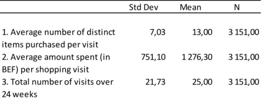
Table 1 shows general statistics for number of items purchased, amount spent and number of visits in the mature market dataset. This information was provided by the author to support data mining results.
Table 1: general statistics - mature market
On average the mature market customer purchased 13 distinct items each time he went to the store. The author informs that most customers bought between 7 and 11 items per shopping visit. The average amount spent per shopping visit is 1.276 Belgian Francs which would be around 31,63 Euros using the last known exchange rate before Belgium joined the Euro Zone in 2002. The average number of visits to the store is 25 over the 5 month period which corresponds to about once per week. The author further informs that most customers visited the store from 4 to 24 times over the entire period.
7.1.2. Emerging Market
Std Dev Mean N
7,03 13,00 3 151,00
751,10 1 276,30 3 151,00
21,73 25,00 3 151,00 1. Average number of distinct
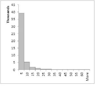
24 Figure 3: average number of distinctive items purchased per visit - emerging market
Results in figure 3 show that the emerging market customer bought 4 distinctive items each time he went to the store during the month. This compares with an average of 13 items per shopping visit of the mature market which means that the emerging market customer buys less product references when he visits the store. This does not necessarily mean that he buys less quantity or value, it could just mean that the mature market customer purchases a wider variety of products when he goes to the store. 91% of the customers bought between 1 and 10 distinctive items per shopping visit during the month. This result compares with the interval between 7 and 11 which is the most frequent interval in the mature market. This difference can be explained by the number of clients in the emerging market coming to the store just to buy one product reference, which is about 35%. There is no indication that these clients are buying large quantities so this should result from economic difficulties.
25 Figure 4 shows that the emerging market customer spends on average 17.500 monetary units each time he visits the store and most customers spend between 1 and 10.000 monetary
units, around 57%. We won’t use a conversion rate to compare the markets otherwise we could be breaking our confidentiality agreement but let us consider a 3 to 1 relationship between mature and emergent markets for comparison purposes. Emerging market customers spend 1 third of what mature markets spend in each visit which is a predictable result since most customers in an emerging market are expected to have low monthly income. To be fair this comparison would have to take prices under consideration since they are also expected to be lower in the emergent market. Knowing that mature market customers go to the store once a week we can use the minimum wage as reference to compare both markets. We conclude that these customers spend around 7% of their weekly income in food retail products while if we apply the same rationale to emergent markets this value is actually higher, around 11%. This could mean that emerging market customers concentrate more of their available income to basic needs. The use of the minimum wage is an attempt to find common ground for comparison purposes. We would need to know which percentage of customers are actually collecting minimum wage to make a more precise comparison between the two markets. We should also mention there is a group of customers buying more than 100.000 monetary units that correspond to 2% of total clients. These may well be the company’s best customers and Management should monitor them closely, encouraging them to return to the store.
Since client ID is not available in the emerging market dataset it’s not possible to compare number of client visits to the store between markets directly. Also we would be comparing a 24 week period to a 4 week period so even if we try to extrapolate the results they
probably wouldn’t be statistically significant. Keeping that in mind we could divide the total number of transactions by the two stores and then by 31 one days, we would get an average of 783 transactions per day. Assuming that the same client doesn’t go to the store twice in the same day we could multiply this number by 7 days of the week and get 5.483 clients per week. Since this is an unusually high number this should indicate that the clients are going to the store more than once a week in the emergent market which is higher than the average of once a week found in the mature market results.
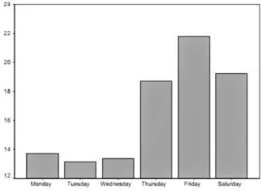
26 From the distribution of daily visits to the store provided in the support document it is clear that in the mature market most visits take place on Thursday, Friday and Saturday as shown in Figure 5. There is no data for Sunday so we are assuming that the store is closed.
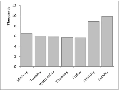
Figure 6: distribution of visits per day of week - emerging market
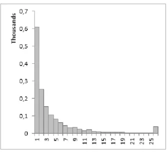
27 Figure 7: inventory turnover - emerging market
Figure 6 shows that 39% of products in the emerging market dataset are slow moving, being sold once or less a day. This is considerably less than the 89% result of the mature market. This difference has several implications ranging from stock management to shelve space. With this kind of numbers for inventory turnover the mature market dataset is expected to have much less fresh products in their offer than the emerging market, otherwise they would be facing serious costs with sell by date products. It is difficult to associate this result to market characteristics as it could be linked to commercial strategies, location and many other factors. On the other hand a bigger offer of fresh products can be linked to emerging markets as they constitute the basic need for a population with lower resources. In some extreme cases customers may not have a refrigerator at home to stock frozen products or the resources to buy anything else than food. Additionally, many emerging countries have agriculture and foreign retailers have to compete with local informal trade in this category if they want to survive in a market where the customer is mainly focused on basic needs.
7.2. POSITIVE ASSOCIATION RULES
7.2.1. Confidence
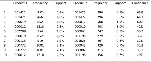
Table 2: top 10 association rules ordered by confidence – emerging market
28 Results in table 2 show strong association rules for the emerging market with confidence values ranging from 29% to 65%. However the association rules support values strike as low for decision making. The rule with highest support has a 1% value which corresponds to about 486 transactions. There are no association rules with more than 2 items in the top 10 and there are 11 different products in the frequent itemsets. Again, these values are in line with the emerging market profile described in the statistics section. With more than 35% of customers buying a
single product in each visit we shouldn’t expect association rules to have high support.
Table 3: top 10 association rules ordered by confidence – emerging market subcategories
There are 10 distinct subcategories in the top 10 association rules of the emerging market as we can observe in table 3. Despite the strongest association rule being found between products belonging to the same subcategory, results show association rules between products of different subcategories for the rest of the top 10.
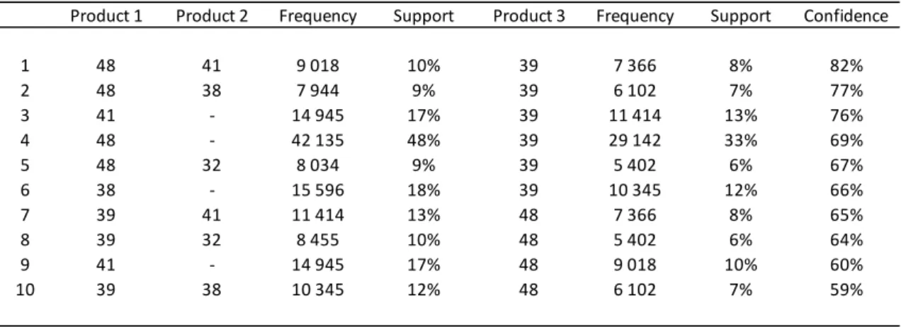
Table 4: top 10 association rules ordered by confidence – mature market
Product 1 Frequency Support Product 2 Frequency Support Confidence
1 001422 452 0,9% 001421 296 0,6% 65%
2 001421 466 1,0% 001422 296 0,6% 64%
3 000019 852 1,8% 000012 508 1,0% 60%
4 000012 1218 2,5% 000019 508 1,0% 42%
5 002288 754 1,6% 000043 247 0,5% 33%
6 000019 852 1,8% 001198 279 0,6% 33%
7 000123 919 1,9% 001626 297 0,6% 32%
8 000772 1001 2,1% 000043 320 0,7% 32%
9 000772 1001 2,1% 000802 313 0,6% 31%
10 000012 1218 2,5% 001198 356 0,7% 29%
Product 1 Subcat Product 2 Subcat Frequency Support Confidence
29 Table 4 shows strong rules at the top 10 for the mature market as well, with confidence values ranging from 59% to 82%. In this market association rules are backed by solid support values, the rule with lowest support in the top 10 has a 7% support value which corresponds to more than 6.000 transactions. Keeping in mind that this result may be influenced by the samples we are using for each market this is a major difference between the datasets that must be registered. There are 4 rules with 3 items in the top 10 which relates to customers buying more references in each visit as described in the statistics section. On the other hand top 10 association rules seem to always revolve around the same items since there are only 5 distinct products in the frequent itemsets.
Table 5: max, min and mean values for support and confidence – emerging market
Table 6: max, min and mean values for support and confidence – mature market
Despite mean values for confidence shown in table 5 and 6 not being too far apart, support values really make a difference in this comparison. This could confirm a significant difference in customer behavior between the emerging and the mature markets reflected in association rules. Economic factors play a very important role in emerging markets and less available income can explain less variety in purchasing decisions. Customers are focused on maximizing the value spent, this means buying basic goods like water, milk and bread for the cheapest value possible. We could also expect more variety in the offering of a mature market supermarket as customers are much more willing to purchase different categories. Supply
Product 1 Product 2 Frequency Support Product 3 Frequency Support Confidence
1 48 41 9 018 10% 39 7 366 8% 82%
2 48 38 7 944 9% 39 6 102 7% 77%
3 41 - 14 945 17% 39 11 414 13% 76%
4 48 - 42 135 48% 39 29 142 33% 69%
5 48 32 8 034 9% 39 5 402 6% 67%
6 38 - 15 596 18% 39 10 345 12% 66%
7 39 41 11 414 13% 48 7 366 8% 65%
8 39 32 8 455 10% 48 5 402 6% 64%
9 41 - 14 945 17% 48 9 018 10% 60%
10 39 38 10 345 12% 48 6 102 7% 59%
Max Min Mean
Confidence 65% 29% 42%
Support 1% 0,5% 0,7%
Max Min Mean
Confidence 82% 59% 69%
30 creates its own demand as a strategy can only work in a market where customers actually have some money to spend.
7.2.2. Lift
Table 7: top 10 association rules ordered by lift – emerging market
Table 7 shows the top 10 association rules ordered by interest measure lift, followed by Leverage and Conviction. Results show lift values ranging from 9,53 to 68,26 for the emerging market. A lift value of 68,26 between products 001422 and 001421 means that it is 68,26 times more likely for a customer to buy product 001421 if he bought product 001422 in the first place, which is quite high. This is an unusual high value but after using two different methods for calculation the result kept unchanged so we considered the value doublechecked. There are no significant differences between the Leverage values of the rules, most of them show a 0,01 value. Conviction ranges from 1,16 to 2,85. In this case rule 7 shows the best result since its 1,16 value means that the rule is expected to make an incorrect prediction 16% of the time.
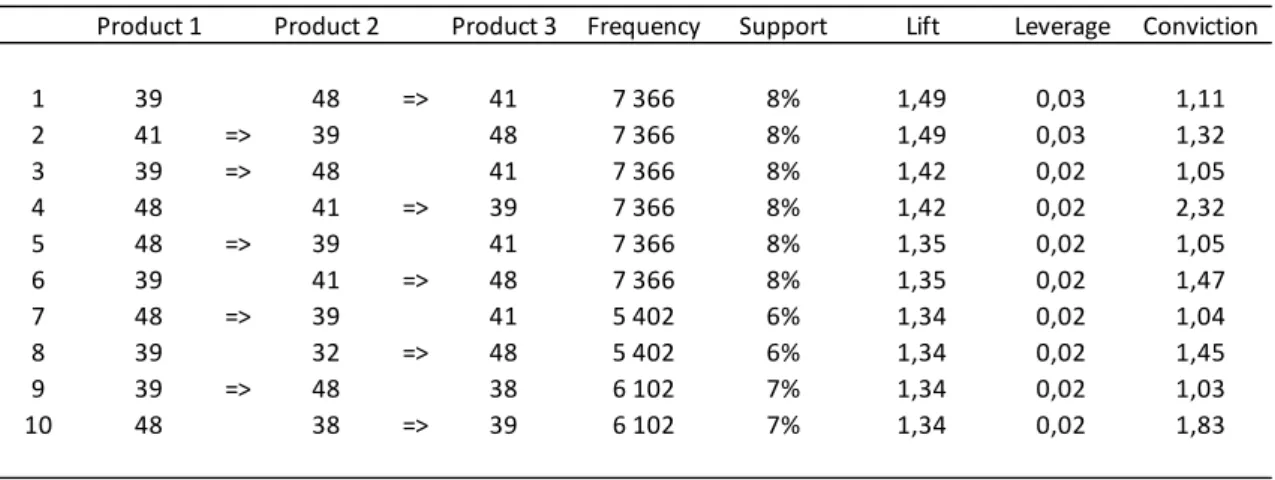
Table 8: top 10 association rules ordered by lift – mature market
Product 1 Product 2 Frequency Support Lift Leverage Conviction
1 001422 001421 296 0,6% 68,26 0,01 2,85
2 001421 001422 296 0,6% 68,26 0,01 2,7
3 000012 000019 508 1,0% 23,78 0,01 1,68
4 000019 000012 508 1,0% 23,78 0,01 2,41
5 001626 000123 297 0,6% 10,65 0,01 1,23
6 000123 001626 297 0,6% 10,65 0,01 1,43
7 000043 002288 247 0,5% 9,76 0 1,16
8 002288 000043 247 0,5% 9,76 0 1,43
9 000043 000772 320 0,7% 9,53 0 1,22
10 000722 000043 320 0,7% 9,53 0,01 1,42
Product 1 Product 2 Product 3 Frequency Support Lift Leverage Conviction
1 39 48 => 41 7 366 8% 1,49 0,03 1,11
2 41 => 39 48 7 366 8% 1,49 0,03 1,32
3 39 => 48 41 7 366 8% 1,42 0,02 1,05
4 48 41 => 39 7 366 8% 1,42 0,02 2,32
5 48 => 39 41 7 366 8% 1,35 0,02 1,05
6 39 41 => 48 7 366 8% 1,35 0,02 1,47
7 48 => 39 41 5 402 6% 1,34 0,02 1,04
8 39 32 => 48 5 402 6% 1,34 0,02 1,45
9 39 => 48 38 6 102 7% 1,34 0,02 1,03
31 As we can observe in table 8 mature market results show lower lift values for the top 10 rules when compared with the emerging market. Values range from 1,34 to 1,49 which is a much smaller amplitude. As already mentioned, top 10 rules are different combinations of the same 5 products so similar values are an expected result. Leverage values are slightly higher in this dataset and Conviction is 1,03 at best. A rule prediction being incorrect only 3% of the time is a much better result than the 16% found in the emerging market. This result is in line with the support and confidence values found in this dataset.
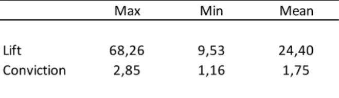
Table 9: max, min and mean values for lift and conviction – emerging market
Table 10: max, min and mean values for lift and conviction – mature market
Table 9 shows an average lift in the emerging dataset of 24,4 which is a much higher value that the 1,39 found in the mature dataset and shown in table 10. Average Conviction is also higher but the difference between both datasets is not so pronounced in this indicator. Overall, the emerging market dataset results show higher lift values for the top 10 rules but the probability of rules making a wrong prediction is also higher.
7.3. NEGATIVE ASSOCIATION RULES
7.3.1. Emerging market
Table 11: product linear correlation within subcategories - emerging market
Max Min Mean
Lift 68,26 9,53 24,40
Conviction 2,85 1,16 1,75
Max Min Mean
Lift 1,49 1,34 1,39
Conviction 2,32 1,03 1,37
Product 1 Product 2 L. Correlation
Sub Category 1 001912 000792 -0,698
Sub Category 2 000802 001720 -0,494
32 We have selected the 10% most frequent items to measure linear correlation between them. Additionally, we identified the products belonging to the same subcategory to ensure we are comparing similar products in search for a substitution effect. Results in table 11 show strong negative correlation between products for the 3 most frequent subcategories. In Subcategory 1 the strongest negative correlation was found between products 001912 and 000792. These items satisfy our frequency criteria, which ensures us that they actually sell, and they belong to the same subcategory so this should be a strong indication of a substitution effect.
Table 12: chi-squared test for contingency tables – subcategories emerging market
The contingency tables show that the substitution effect occurred in 99% of the transactions where at least one of the items was present as we can observe in table 12. This result holds for all of the 3 pairs of items that we analyzed. The Chi Squared test for contingency tables confirms these results showing a statistically significant negative relationship between the items. We should expect the existence of strong substitution effects in emerging markets since the strategic positioning of companies are mainly price driven. A customer with lower economic resources is expected to be very sensitive to price variations as they have a big impact in his disposable income. This translates to buying just one item to suppress each basic need and to switch between similar products whenever the price changes, which would explain the substitution effect.
7.3.2. Mature market
Table 13: k-medoids clusters - mature market
Table 13 shows the results after running the k-medoids algorithm with 3 clusters set beforehand. Increasing the number of clusters generated more groups but with similar characteristics so we consider 3 clusters to be the ideal option. Frequency and Sales Reason
Product 1 Product 2 Frequency Chi-Square Prob
Sub Category 1 001912 000792 98,8% 99,08 0,000
Sub Category 2 000802 001720 99,4% 29,25 0,000
Sub Category 3 001288 002829 99,3% 7,05 0,008
Cluster Centroid Frequency Sales Reason Avg Add Item
Cluster 1 694 0,005 0,007 13,25
Cluster 2 1513 0,005 0,005 16,107
33 show closer values between clusters therefore we consider Average Additional Items to be the variable with more distinctive power. Cluster 3 is the cluster with highest Average Additional Items value. On average, when an item of this cluster is bought there are 18 more items in the basket. Results show a Frequency ranging between 0,2% and 0,5% of total transactions and Sales Reason ranging between 0,5% and 0,7%. Cluster 1 is one of the most frequent along with Cluster 2 and shows the highest Sales Reason value, which means this is the cluster with more clients going to the store just to buy a single product.
Figure 8: k-medoids clusters – mature market
Figure 6 illustrates the 3 Clusters returned by the k-medoids algorithm using Average Additional Item and Sales Reason for X and Y coordinates respectively. Data visualization confirms the existence of 3 well defined, distinct Clusters that we can use as an alternative to
group similar products. Since we don’t have subcategory information available for the mature
market we will use the segmentation results as the similarity criteria required to identify negative associations between products.
Table 14: product linear correlation within clusters - mature market
Following the same procedure that was used for subcategories, we have selected the 10% more frequent items, identified which cluster they belong to and measured linear
Product 1 Product 2 L. Correlation
Cluster 1 271 170 -0,043
Cluster 2 475 310 -0,048
34 correlation within clusters. Table 14 shows products with higher negative correlation for each cluster. The highest negative association was found in Cluster 2 between products 475 and 310 showing a -0,048 result. These two products satisfy the frequency criteria and belong to the same cluster so this should be an indication of a potential substitution effect.
Table 15: chi-squared test for contingency tables - clusters mature market
The Chi-squared test for contingency tables confirms the results for Cluster 1, 2 and 3, guaranteeing statistical significance of the negative relationship. The substitute effect occurred in almost every transaction where at least one of the products was present as shown in table 15.
7.3.3. Emerging market vs Mature market
Results confirm the existence of potential substitution effects both for emerging and mature markets. Negative associations seem to be stronger in the emerging market but we should keep in mind that we are using an alternative method to find similar products in the mature market. Applying the same alternative method to the emerging market could help us extend our analysis using the results as additional distinctive criteria between the two markets. Table 16: k-medoids clusters - emerging market
While running the k-medoids algorithm for the emerging market dataset 4 was found to be the ideal number of clusters to guarantee well defined, distinct groups. This compares with the 3 clusters option used in the mature market segmentation. Frequency ranges from 0,3% of transactions of Cluster 2 to 0,5% of transactions of Cluster 1 which was found to be the most
Product 1 Product 2 Frequency Chi-Square Prob
Cluster 1 271 170 98.9% 75,052 0,000
Cluster 2 475 310 99.6% 101,258 0,000
Cluster 3 76 1144 99.6% 16,833 0,000
Cluster Centroid Frequency Sales Reason Avg Add Item
Cluster 1 000078 0,005 0,027 26,246
Cluster 2 000256 0,003 0,066 13,607
Cluster 3 000840 0,004 0,045 18,795
35 frequent Cluster. Table 16 shows Cluster 4 with the highest Sales Reason result with almost 15% of the transactions containing a single item. This is considerably higher than the results found in the mature market. Despite the number of transactions containing a single item being considerably higher in the emerging market as already discussed, the Average Additional Items indicator shows Cluster 1 as a group of products that is bought with 26 other items in the basket on average. This value is considerably higher than the 18 additional items of Cluster 3 found in the mature market, which is the highest value for that dataset.
Figure 9: k-medoids clusters – emerging market
Figure 7 illustrates the 4 clusters returned by the k-medoids algorithm using Average Additional Items and Sales Reason for X and Y coordinates respectively. Again, data visualization confirms the existence of 4 well defined, distinct groups of products using transaction related variables for segmentation.
Table 17: cluster comparison - centroids
Using centroids of each cluster for comparison, the closest match we could find between the two markets was Cluster 3 and Cluster 2 of the emerging and mature market, respectively. Despite variables Frequency and Average Additional Items results not being too far apart Sales Reason shows a considerably different behavior in the two datasets as already discussed. This
Cluster Centroid Frequency Sales Reason Avg Add Item
E-Cluster 3 000840 0,004 0,045 18,795
37 8. CONCLUSIONS
Overall, results confirm a different customer profile between markets and these differences are reflected in the positive and negative association rules found in the datasets. The differences in customer behavior seem to be related to market specific cultural and economic characteristics.
The emergent market customer buys less references than the mature market customer when he visits the store and there is a considerable number of clients buying just one product reference in each visit. The value spent in each visit is about one third of the value spent by the mature market customer but we suspect the percentage of monthly income he spends in food retail is higher. Both customers prefer to go shopping closer to the weekend but Monday is the third preferred option for the emerging market customer. The mature market customer prefers Thursdays along with Friday and Saturday. We believe that results showing Monday as a frequent shopping day can be related to weekly organized labor, which is a common practice in emerging economies. The emerging market results shows a steadier flow of customers going to the store along the week while customer visits in mature markets seem to be highly concentrated around the weekend. This is a relevant difference since companies operating in emerging markets are expected to have a steadier cash flow. Results indicate less fresh products in the mature market offer but this cannot be directly linked to a customer profile since it could result from a number of other factors like commercial strategies or location of the store.
The emerging market shows strong association rules in the top 10 but the values strike as low to support decision making when compared to the solid statistical significance found in the mature markets. The considerable number of clients buying just one item found in the emerging market explains these results. Baskets with more than one item are not as frequent as in the emergent market so we should expect lower support for the association rules. A basket with fewer items is an indication of a different purchasing behavior between the two markets that may be related to economic resources. Although the strongest rule was found between items of the same subcategory the emerging market shows a considerable number of association rules with items belonging to different subcategories. This is an interesting result since rules between items of different subcategories are more likely to constitute new knowledge for the company. This may indicate the existence of not so obvious combinations between products that management can try to benefit from. Rules between items of the same subcategory may result from kits, promotion packs, campaigns or other intentional well-known product combinations. We didn’t have access to the product hierarchy of the mature market but rules seem to revolve around the same 5 items that are expected to be best sellers.
38 markets using segmentation as an alternative grouping method, we concluded that there is also an indication of the existence of substitution effects in the mature market but the negative relationships found between products seem to be stronger in the emergent market.
39 9. REFERENCES
Agrawal, R., Imielinski, T., & Swami, A. (1993). Mining association rules between sets of items in large databases. ACM SIGMOD Record, 22(May), 207–216.
http://doi.org/10.1145/170036.170072
Agrawal, R., & Srikant, R. (1994). Fast algorithms for mining association rules. Proceedings of the 20th International Conference on Very Large Databases, 487–499.
Agrawal, R., & Srikant, R. (1995). Mining sequential patterns. Proc. of the 11th Int. Conf. on Data Engineering, 3–14. http://doi.org/10.1016/j.jbi.2007.05.004
Bonchi, F., Giannotti, F., Mazzanti, A., & Pedreschi, D. (2003). ExAnte : Anticipated Data
Reduction in Constrained Pattern Mining. Knowledge Discovery in Databases: PKDD 2003, 59–70.
Brin, S., Motwani, R., & Silverstein, C. (1997). Beyond market baskets: generalizing association rules to correlations. ACM SIGMOD Record, 26(2), 265–276.
http://doi.org/10.1145/253262.253327
Dawar, N., & Chattopadhyay, A. (2002). Rethinking marketing programs for emerging markets.
Long Range Planning, 35(5), 457–474. http://doi.org/10.1016/S0024-6301(02)00108-5 Grahne, G., & Zhu, J. (2003). Efficiently Using Prefix-trees in Mining Frequent Itemsets. Proc. of
the 1st IEEE ICDM Workshop on Frequent Itemset Mining Implementations, 236--245. Retrieved from
ftp://ftp.cse.buffalo.edu/users/azhang/disc/disc01/cd1/out/websites/dmkd/pei.pdf%5Cn http://ftp.informatik.rwth-aachen.de/Publications/CEUR-WS/Vol-90/grahne.pdf
Han, J., Cheng, H., Xin, D., & Yan, X. (2007). Frequent pattern mining: Current status and future directions. Data Mining and Knowledge Discovery, 15(1), 55–86.
http://doi.org/10.1007/s10618-006-0059-1
Han, J., Chiang, J., & Kamber, M. (1997). Metarule-Guided Mining of Multi-Dimensional Association Rules Using Data Cubes. Proceedings ACM SIGKDD Int’l Conf. Knowledge
Discovery and Data Mining, 207–210.
Han, J., & Fu, Y. (1995). Discovery of Multiple-Level Association Large Databases School of Computing Science. Proceedings of the 21st VLDB Conference Zurich, Swizerland, 420– 431.
Han, J., & Kamber, M. (2011). Data mining: concepts and techniques. Elsevier/Morgan Kaufmann.
Han, J., Pei, J., & Yin, Y. (2000). Mining Frequent Patterns without Candidate Generation.
Networks, 1–12.
International Monetary Fund. (2015). World Economic Outlook. Retrieved from http://www.imf.org/external/pubs/ft/weo/2015/02/pdf/text.pdf
Klemettinen, M., & Mannila, H. (1994). Finding interesting rules from large sets of discovered association rules. Proceedings of the Third International Conference on Information and Knowledge Management.
40
productivity. McKinsey Global Institute.
Newman, K. L., & Nollen, S. D. (1996). Culture and Congruence: The Fit between Management Practices and National Culture. Journal of International Business Studies, 27(4), 753–779. Pan, F., Cong, G., Tung, A. K. H., Yang, J., & Zaki, M. J. (2003). CARPENTER: Finding Closed
Patterns in Long Biological Datasets. Ninth ACM SIGKDD International Conference on Knowledge Discovery and Data Mining, 637–642. http://doi.org/10.1145/956750.956832 Solow, R. M. (1956). A contribution to the theory of economic growth. The Quarterly Journal of
Economics, 65–94.
Sriknat, R., & Agrawal, R. (1996). Agrawal.Mining Quantitative Association Rules in Large Relational Tables. ACM SIGMOD on Management of Data.
Sullivan, A., & Sheffrin, S. (2003). Economics: Principles in action. New Jersey: Pearson Prentice Hall.
Washio, T., & Motoda, H. (2003). State of the art of graph-based data mining. ACM SIGKDD Explorations Newsletter, 5(1), 59. http://doi.org/10.1145/959242.959249
Xin, D., Han, J., Yan, X., & Cheng, H. (2005). Mining compressed frequent-pattern sets. Vldb, 709. Retrieved from http://portal.acm.org/citation.cfm?id=1083675
Yan, X., Han, J., & Afshar, R. (2003). CloSpan: Mining: Closed Sequential Patterns in Large Datasets. Proceedings of the 2003 SIAM International Conference on Data Mining, 166– 177.
Zaki, M. J. (2000). Scalable algorithms for association mining. IEEE Transactions on Knowledge and Data Engineering, 12(3), 372–390. http://doi.org/10.1109/69.846291