Journal of Engineering Science and Technology Review 6 (4) (2013) 45-52 Special Issue on Recent Advances in Nonlinear Circuits: Theory and Applications
Research Article
Analysis and Anti-Synchronization of a Novel Chaotic System via Active and Adaptive
Controllers
V. Sundarapandian*
Research and Development Centre, Vel Tech University, Avadi, Chennai-600 062, Tamil Nadu, INDIA
Received 30 May 2013; Revised 4 September 2013; Accepted 25 September 2013
___________________________________________________________________________________________
Abstract
Anti-synchronization of chaotic systems deals with the problem of asymptotically synchronizing the sum of states of a pair of chaotic systems called master and slave systems with the help of controllers attached to the slave system. When two chaotic systems are anti-synchronized, then their states are asymptotically equal in magnitude, but opposite in phase. Anti-synchronization of chaotic systems has applications in many engineering areas such as secure communications, secure data encryption, cryptosystems, etc. This paper announces a novel 3-D chaotic system and describes its qualitative properties. Next, this paper deals with the design of active and adaptive controllers for synchronizing the states of identical novel chaotic systems. Active controllers are used when the system parameters are available for measurement and the synchronization result is established using Lyapunov stability theory. Adaptive controllers are used when the system parameters are unknown. In this case, estimates are used in lieu of the unknown system parameters and adaptive controllers are designed using adaptive control theory and Lyapunov stability theory. Numerical simulations using MATLAB have been shown to demonstrate the proposed active and adaptive synchronization results for novel chaotic systems.
Keywords: Chaos, chaotic attractors, anti-synchronization, active control, adaptive control.
__________________________________________________________________________________________
1. Introduction
Chaotic systems are typically defined as nonlinear dynamical systems which are sensitive to initial conditions and which have at least one positive Lyapunov exponent. The first experimentally verified chaotic system was due to Lorenz [1] in 1963, while he was modelling weather patterns with a 3-D nonlinear model.
In the chaos literature, there are many paradigms of 3-D chaotic systems such as Rössler system [2], Rabinovich system [3], Arneodo-Coullet system [4], Shimizu-Morioka system [5], Colpitt’s oscillator [6], Shaw system [7], Chua circuit [8], Ruckildge system [9], Sprott systems [10], Chen system [11], Lü-Chen system [12], Chen-Lee system [13], Tigan system [14], Cai system [15], Li system [16], Wang system [17], Harb system [18], Sundarapandian system [19], Gissinger system [20], etc.
In this research work, we describe a novel 8-term 3-D chaotic system having three quadratic nonlinearities. We describe the properties of the novel chaotic system. We also derive the Lyapunov exponents and Kaplan-Yorke dimension of the novel chaotic system. The maximal Lyapunov exponent (MLE) for the novel chaotic system is found as
1=5.0894,
L which is a large value for a polynomial chaotic system. Thus, the novel chaotic system discovered in this work shows strong chaotic behaviour.
In the last few decades, chaos control and synchronization have been applied to several branches of science and engineering such as lasers [21, 22], electronic devices [23, 24], chemical reactions [25, 26], ecology [27, 28], secure communications [29, 30], robotics [31, 32], forecasting [33, 34], cryptosystems [35, 36], neural networks [37, 38], finance [39, 40], etc. Anti-synchronization has been applied to several areas like neural networks [41, 42], coupling [43], lattices [44], oscillators [45], pattern recognition [46], etc.
Anti-synchronization of chaotic systems deals with a pair of chaotic systems connected in series, called as master and slave systems, and the problem can be described as finding a feedback control law using the states of master and slave chaotic systems so that the sum of their respective states decays to zero asymptotically with time. In other words, when anti-synchronization occurs asymptotically, the respective states of the master and slave systems will be equal in magnitude and opposite in phase.
Various design techniques have been proposed for the
J
estr
JOURNAL OF Engineering Science andTechnology Review
www.jestr.org
anti-synchronization of chaotic systems such as active control [47-50], adaptive control [51-53], sliding mode control [54-55], etc.
Active control method is used for anti-synchronizing identical novel chaotic systems, when the system parameters are available for measurement. When the system parameters are not known, adaptive control method is used for anti-synchronizing novel chaotic systems and feedback control laws are devised using estimates of the unknown system parameters and parameter update laws are derived using Lyapunov stability theory [56].
This research work is organized as follows. Section 2 describes the 8-term novel chaotic system with three quadratic nonlinearities. The phase portraits of the novel chaotic system are depicted in this section. Section 3 describes a detailed qualitative analysis and properties of the novel chaotic system. Section 4 describes the active controller design for the anti-synchronization design of the identical novel chaotic systems with known system parameters. Section 5 describes the adaptive controller design for the anti-synchronization of the identical novel chaotic systems with unknown system parameters. Section 6 concludes this research work with a summary of the main results.
2. A Novel Chaotic System
In this section, we describe a novel 8-term chaotic system having three quadratic nonlinearities.
The novel system is defined by the 3-D dynamics
! x
1=a(x2−x1)+x2x3 !
x
2=bx1+cx2−x1x3 !
x
3=−dx3+x1 2
(1)
where x x1, 2,x3 are states and a b c d, , , are constant, positive, parameters of the system (1).
We note that the system (1) has 8 terms on the R.H.S. and a quadratic nonlinearity in each of the equations describing the system.
The system (1) exhibits a strange chaotic attractor for the parameter values
21.5, 20.6, 11, 6.4
= = = =
a b c d (2)
For numerical simulations, we have used classical fourth-order Runge-Kutta method (MATLAB) for solving the system (1) when the initial conditions are chosen as
1(0) 0.5, (0)= 2 =2.1, (0) 1.83 =
x x x
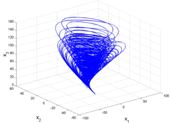
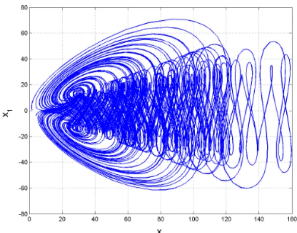
Fig. 1 depicts the strange attractor of the novel chaotic system (1) in 3-D view, while Figs. 2, 3 and 4 depict the 2-D projection of the system (1) in ( ,x x1 2),
2 3
( , )x x and ( , )x3 x1 plane, respectively.
Fig. 1. Strange attractor of the novel chaotic system.
Fig. 2. A 2-D projection of the novel system in the ( ,x1 x2)−plane.
Fig. 4. A 2-D projection of the novel system in the (x3,x1)−plane.
3. Analysis of the Novel Chaotic System with Three Quadratic Nonlinearities
A. Dissipativity
In vector notation, the novel chaotic system (1) can be expressed as
!
x= f (x)= f1(x)
f2(x)
f3(x) !
" # # # #
$
% & & & &
(3)
The divergence of the vector field f on R3is given by
1 2 3
1 2 3
( ) ( ) ( )
div( ) ∂ ∂ ∂
∇ ⋅ = = + +
∂ ∂ ∂
f x f x f x
f f
x x x (4)
We know that ∇ ⋅f measures the rate at which the
volumes change under the flow Φtof f.
Let D be any given region in R3with a smooth boundary. Let D t( )=Φt( ).D Also, let V t( )denotes the volume of
( ). D t
By Liouville’s theorem, we have
( ) ( )
( ) =
∫
∇ ⋅D t
dV t
f dx dy dz
dt (5)
Using the equation (1) of the novel system (A), we find that
1 2 3
1 2 3
( ) 0
∂ ∂ ∂
∇ ⋅ = + + =− + − <
∂ ∂ ∂
f f f
f a d c
x x x (6)
if the positive constants a, c and d satisfy the condition that
+ >
a d c (7)
We note that for the system parameters defined in Eq. (2), the condition (7) is met.
Thus, it follows that
0
∇ ⋅f =−µ< (9)
By substituting the value of ∇ ⋅f in Eq. (5), we get
( ) ( )
( )
=−
∫
=−D t dV t
dx dy dz V t
dt µ µ (10)
Solving the linear differential equation (10), we get the solution
(
)
( )= (0)exp −V t V
µ
t (11)From Eq. (11), it follows that any volume V t( ) must
shrink to zero exponentially as t→ ∞. Thus, the novel chaotic system (1) is a dissipative chaotic system, when the parameters are chosen as in (2). Hence, the asymptotic motion of the novel system settles onto a strange attractor.
B. Equilibrium Points
We obtain the equilibrium points of the novel chaotic system by solving the nonlinear system of equations
( )=0
f x (12)
We take the parameter values as in the chaotic case, viz.
21.5, 20.6, 11, 6.4
= = = =
a b c d (13)
Then the equilibrium points of the novel chaotic system are obtained numerically using MATLAB as
0
1
: (0,0,0)
: (12.8048, 5.8427, 25.6192) E
E (14)
Using the first method of Lyapunov, it is easy to see that E0 is a saddle point and E1 is a saddle focus point. Hence, all the equilibrium points of the novel chaotic system are unstable.
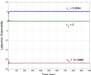
C. Lyapunov Exponents
We take the initial state as
1(0) 0.5, (0)= 2 =2.1, (0) 1.83 =
x x x (15)
We take the parameters as given in (13). Then the Lyapunov exponents of the novel chaotic system (1) are obtained numerically using MATLAB as
1=5.0894, 2=0, 3=−21.9465
L L L (16)
This shows mathematically that the novel system (A) is indeed chaotic. Note that the maximal Lyapunov exponent (MLE) of the novel system is L1=5.0894,which a large value for a polynomial chaotic system is. Thus, the novel system depicts strong chaotic behaviour.
Fig. 5. Dynamics of the Lyapunov exponents of the novel system.
D. Kaplan-Yorke Dimension
The Kaplan-Yorke dimension of the system (A) is
1 2
1
1 3
1
2 2.2319
| | | |
j
KY i
i j
L L
D j L
L+ = L
+
= +
∑
= + = (17)Eq. (17) shows that the novel chaotic system (1) is a dissipative system and the Kaplan-Yorke dimension of the system is fractional.
4. Active Controller Design for the Anti-Synchronization of Novel Chaotic Systems
In this section, we derive new results for the active controller for the anti-synchronization of the identical novel chaotic systems introduced in this paper. The main result of this section is established using Lyapunov stability theory [56].
As the master (or drive) system, we consider the novel chaotic system given by
! x
1=a(x2−x1)+x2x3 !
x
2=bx1+cx2−x1x3 !
x
3=−dx3+x1 2
(18)
where x x1, 2,x3are the states and a b c d, , , are known system parameters.
As the slave (or response) system, we consider the controlled novel chaotic system given by
!
y1=a(y2−y1)+y2y3+u1
!
y2=by1+cy2−y1y3+u2
!
y3=−dy3+y12+u3
(19)
where y y y1, 2, 3 are the states and u u1, 2,u3 are active controllers to be designed.
The anti-synchronization error between the chaotic systems (18) and (19) is defined as
1 1 1
2 2 2
3 3 3
= +
= +
= +
e y x
e y x
e y x
(20)
The error dynamics is calculated as
!
e1=a(e2−e1)+y2y3+x2x3+u1
!
e2=be1+ce2−y1y3−x1x3+u2
!
e3=−de3+y12+x12+u3
(21)
Next, we introduce the active controller defined by
1 2 1 2 3 2 3 1 1
2 1 2 1 3 1 3 2 2
2 2
3 3 1 1 3 3
( )
=− − − − −
=− − + + −
= − − −
u a e e y y x x k e
u be ce y y x x k e
u de y x k e
(22)
where k k1, 2,k3are positive gains.
By substituting the control law (22) into (21), we get the closed-loop error dynamics as
!
e 1=−k1e1 ! e
2=−k2e2
!
e 3=−k3e3
(23)
Next, we prove the main result of this section.
Theorem 1. The active nonlinear controller defined by (22) achieves global and exponential anti-synchronization of the identical novel chaotic systems described by the equations (18) and (19), where ki,(i=1,2,3)are positive constants.
Proof. The proof is an application of the Lyapunov stability theory [56].
We consider the Lyapunov function V defined by
(
2 2 2)
1 2 3
1
, 2
= + +
V e e e (24)
which is quadratic and positive definite on R3.
Differentiating V along the trajectories of the closed-loop error dynamics (23), we get
2 2 2
1 1 2 2 3 3,
=− − −
&
V k e k e k e (25)
which is a quadratic and negative definite function on R3. Hence, by Lyapunov stability theory [56], the anti-synchronization errors globally and exponentially converge to zero with time.
This completes the proof. !
For numerical simulations, the classical fourth order Runge-Kutta method with step size h=10−8has been used with MATLAB to solve the novel chaotic systems (18) and (19) when the active controller (22) is applied.
We take the positive gains kias ki=5,(i=1,2,3).
The values of the system parameters for the novel chaotic systems (18) and (19) are taken as in the chaotic case, viz.
21.5, 20.6, 11, 6.4
= = = =
a b c d
The initial state of the master system (18) is taken as
1(0) 5.4, (0)= 2 =−1.8, (0)3 =7.2
The initial state of the slave system (19) is taken as
1(0) 1.2, (0)= 2 =−9.7, (0) 3.63 =
y y y
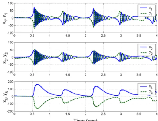
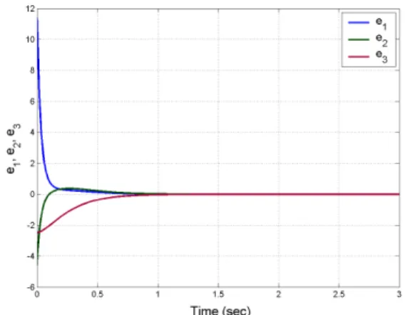
Fig. 6 depicts the anti-synchronization of the identical novel chaotic systems described by the equations (18) and (19), while Fig. 7 depicts the time history of the anti-synchronization errors e t1( ), ( ), ( ).e2t e3t
Fig. 6. Anti-synchronization of the identical novel chaotic systems.
Fig. 7. Time history of the anti-synchronization errors e1( ),t e2( ),t e3( )t .
5. Adaptive Controller Design for the Anti-Synchronization of Novel Chaotic Systems
In this section, we derive new results for the adaptive controller for the anti-synchronization of the identical novel chaotic systems with unknown parameters. The adaptive controller design is carried out using estimates of the unknown parameters and Lyapunov stability theory [56].
As the master (or drive) system, we consider the novel chaotic system given by
! x
1=a(x2−x1)+x2x3
!
x
2=bx1+cx2−x1x3 !
x
3=−dx3+x1 2
(26)
controlled novel chaotic system given by
!
y1=a(y2−y1)+y2y3+u1
!
y2=by1+cy2−y1y3+u2
!
y3=−dy3+y12+u3
(27)
where y y y1, 2, 3are the states and u u1, 2,u3 are adaptive
controllers to be designed.
We define the anti-synchronization error between the systems (26) and (27) as
1 1 1
2 2 2
3 3 3
= +
= +
= +
e y x
e y x
e y x
(28)
The error dynamics is calculated as
!
e1=a(e2−e1)+y2y3+x2x3+u1
!
e2=be1+ce2−y1y3−x1x3+u2
!
e3=−de3+y12+x12+u3
(29)
Next, we introduce the adaptive controller defined by
1 2 1 2 3 2 3 1 1
2 1 2 1 3 1 3 2 2
2 2
3 3 1 1 3 3
( ) ( )( )
( ) ( ) ( )
( ) ( )
=− − − − −
=− − + + −
= − − −
u t A t e e y y x x k e
u t B t e C t e y y x x k e
u t D t e y x k e
(30)
where A(t), B(t), C(t), D(t) are estimates of the unknown system parameters a, b, c, d respectively, and k k1, 2,k3are positive gains.
By substituting the control law (30) into (29), we get the closed-loop error dynamics as
! e
1=(a−A(t))(e2−e1)−k1e1 !
e
2=(b−B(t))e1+(c−C(t))e2−k2e2
!
e
3=−(d −D(t))e3−k3e3 (31)
We define the errors in estimating parameters of the novel system as
( ) ( )
( ) ( )
( ) ( )
( ) ( )
= −
= −
= −
= −
a
b
c
d
e t a A t
e t b B t
e t c C t
e t d D t
(32)
Differentiating (32) with respect to t we obtain
! e
a(t)=− ! A(t)
! e
b(t)=−
! B(t)
! e
c(t)=− ! C(t)
! e
d(t)=− ! D(t)
!
e
1=ea(e2−e1)−k1e1 !
e
2=ebe1+ece2−k2e2 !
e
3=−ede3−k3e3
(34)
Next, we derive an update law for the parameter estimates using Lyapunov stability theory. We take a candidate Lyapunov function defined by
(
2 2 2 2 2 2 2)
1 2 3
1
, 2
= + + + a+ b+ c+ d
V e e e e e e e (35)
which is a quadratic and positive-definite function on R7. Next, we calculate the time-derivative of V along the trajectories of (33) and (34). We obtain
!
V =−k
1e1 2
−k
2e2 2
−k
3e3 2
+ea e
1(e2−e1)−
! A
"
# $%+eb e1e2− !
B
" # $%
+e c e2
2−C!
"
#& $%'+ed −e3
2− !
D
" #& $%'
(36)
To guarantee global exponential stability of the systems (33) and (34), we need to choose parameter updates carefully so that V&is a quadratic, negative definite function on R7.
Thus, we choose the parameter update law as follows:
! A=e
1(e2−e1)+k4ea !
B=e
1e2+k5eb !
C =e 2
2 +k
6ec !
D=−e 3 2
+k 7ed
(37)
where k4,k5,k6,k7are positive constants.
Next, we prove the main result of this section.
Theorem 2. The adaptive controller defined by (33) and the parameter update law defined by (37) achieve global and exponential anti-synchronization of the identical novel chaotic systems unknown parameters described by the equations (26) and (27), where ki,(i=1,K,7)are positive
constants. The parameter estimation errors ( ), ( ), ( ), ( )
a b c d
e t e t e t e t exponentially converge to zero with
time.
Proof. The assertions are established using Lyapunov stability theory [56].
We have already noted that the Lyapunov function V defined by (35) is quadratic and positive definite on R7.
Next, we substitute the parameter update law defined by (37) into the dynamics (36). Thus, the dynamics (36) is simplified as:
! V =−k
1e1 2
−k 2e2
2 −k
3e3 2
−k 4ea
2 −k
5eb 2
−k 6ec
2 −k
7ed 2
(38)
which is a quadratic and negative definite function on R7. Hence, by Lyapunov stability theory [56], the anti-synchronization and parameter estimation errors globally and exponentially converge to zero with time.
This completes the proof. !
For numerical simulations, the classical fourth order Runge-Kutta method with step size h=10−8has been used with MATLAB to solve the chaotic systems (26) and (27) when the adaptive controller (30) and the parameter update law (37) are applied.
We take the positive gains kias ki=5,(i=1,K,7). The values of the system parameters for the systems (26) and (27) are taken as in the chaotic case, viz.
21.5, 20.6, 11, 6.4
= = = =
a b c d
The initial state of the master system (26) is taken as
1(0) 5.3, (0)= 2 =4.1, (0)3 =−3.8
x x x
The initial state of the slave system (27) is taken as
1(0)=6.1, (0)2 =−8.7, (0) 1.33 =
y y y
The initial values of the parameter estimates are taken as
(0)=3.6, (0)=5.9, (0)=2.2, (0) 10.5=
A B C D
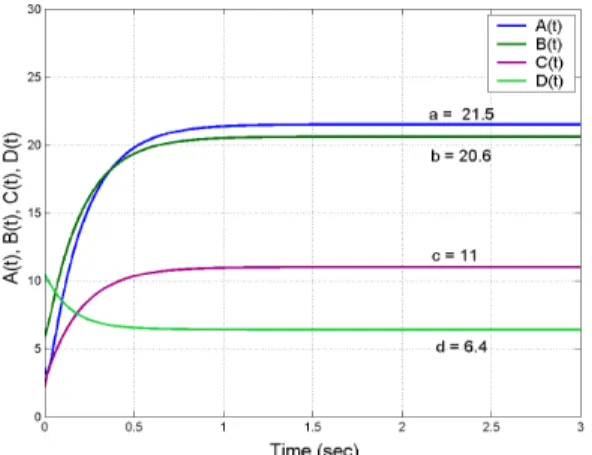
Fig. 8 depicts the anti- synchronization of the identical novel chaotic systems described by the equations (26) and (27), while Fig. 9 depicts the time history of the anti-synchronization errors e t1( ), ( ), ( ).e2t e3t Also, Fig.10 depicts the time history of the parameter estimates
( ), ( ), ( ), ( )
A t B t C t D t and Fig 11 depicts the time history of
the parameter estimation errors ea( ), ( ), ( ),t e t e t eb c d( ).t
Fig. 8. Anti-synchronization of the novel chaotic systems.
Fig. 10. Time history of the parameter estimates A t( ), ( ), ( ), ( )B t C t D t .
Fig. 11. Time history of the parameter estimation errors ( ), ( ), ( ), ( ).
a b c d
e t e t e t e t
6. Conclusion
In this research work, we have derived a novel 3-dimensional 8-term polynomial chaotic system with three quadratic nonlinearities. First, we provided a detailed qualitative analysis of the novel chaotic system and described its properties. Next, we calculated the Lyapunov exponents and Kaplan-Yorke dimension of the novel chaotic system. We found that the maximal Lyapunov exponent (MLE) for the novel chaotic system is L1=5.0894,which is a large value for a polynomial chaotic system. Next, using the Lyapunov stability theory, we have derived active and adaptive controllers for the identical novel chaotic systems having known and unknown system parameters, respectively. MATLAB plots were shown to illustrate the active and adaptive controller designs for the anti-synchronization of identical novel chaotic systems.
______________________________ References
1. E.N. Lorenz, J. Atmospheric Sci. 20, 130 (1963). 2. O.E. Rössler, Phy. Lett. 57A, 397 (1976).
3. M.I. Rabinovich, and A.L. Fabrikant, Sov. Phys. JETP. 50, 311 (1979).
4. A. Arneodo, P. Coullet, and C. Tresser, Phys. Lett. A. 79, 259 (1980).
5. T. Shimizu, and N. Morioka, Phy. Lett. A. 76, 201 (1980). 6. M.P. Kennedy, IEEE Trans. Circuits Sys. 41, 771 (1994). 7. R. Shaw, Zeitschrift für Natur. 36, 80 (1981).
8. L.O. Chua, T. Matsumoto, and M. Komuro, IEEE Trans. Circuits Sys. 32, 798 (1985).
9. A.M. Rucklidge, J. Fluid Mech. 237, 209 (1992). 10. J.C. Sprott, Phys. Rev. E, 50, 647 (1994).
11. G. Chen, and T. Ueta, Internat. J. Bifur. Chaos. 9, 1465 (1999). 12. J. Lü, and G. Chen, Internat. J. Bifur. Chaos. 12, 659 (2002). 13. H.K. Chen, and C.I. Lee, Chaos, Solit. Fract. 21, 957 (2004). 14. G. Tigan, and D. Opris, Chaos, Solit. Fract. 36, 1315 (2008). 15. G. Cai, and Z. Tan, J. Uncertain Sys. 1, 235 (2007). 16. D. Li, Phy. Lett. A. 372, 387 (2008).
17. L. Wang, Nonlinear Dyn. 56, 453 (2009).
18. A.M. Harb, B.A. Harb, Chaos, Solit. Fract. 20, 719 (2004). 19. V. Sundarapandian, and I. Pehlivan, Math. Computer Modelling.
55, 1904 (2012).
20. C. Gissinger, Euro. Phys. J. B. 85, 3667 (2012).
21. E.M. Shahverdiev, and K.A. Shore, Optics Commun. 282, 3568 (2009).
22. Q. Yang, Z.M. Wu, J.G. Wu, and G.Q. Xia, Optics Commun. 281, 5025 (2008).
25. A. Shabunin, V. Astakhov, V. Demidov, A. Provata, F. Baras, G. Nicolis, and V. Anishchenko, Chaos, Solit. Fract. 15, 395 (2003). 26. Q.S. Li, and R. Zhu, Chaos, Solit. Fract. 19, 195 (2004). 27. R. Engbert, and F.R. Drepper, Chaos, Solit. Fract. 4, 1147 (1994). 28. I. Suárez, Ecology. 117, 305 (1999).
29. J. Zhou, H.B. Huang, G.X. Qi, P. Yang, and X. Xie, Phy. Lett. A.
335, 191 (2005).
30. G. Kaddoum, M. Coulon, D. Roviras, and P. Chargé, Signal Processing. 90, 2923 (2010).
31. U. Nechmzow, and K. Walker, Robo. Auto. Sys. 53, 177 (2005). 32. B.H. Kaygisiz, I. Erkmen, and A.M. Erkmen, Chaos, Solit. Fract.
29, 148 (2006).
33. H. Cheng, and A. Sandu, Env. Model. Soft. 24, 917 (2009). 34. H. Yuxia, and Z. Hongtao, Physics Procedia. 25, 588 (2012). 35. M. Usama, M.K. Khan, K. Algathbar, and C. Lee, Comp. Math.
Appl. 60, 326 (2010).
36. H. Hermassi, R. Rhouma, and S. Belghith, J. Sys. Soft. 85, 2133 (2012).
37. G. He, Z. Cao, P. Zhu, and H. Ogura, Neural Networks. 16, 1195 (2003).
38. E. Kaslik, and S. Sivasundaram, Neural Networks, 32, 245 (2012). 39. J.C. Sprott. Phy. Lett. A. 325, 329 (2004).
40. D. Guégan, Annual Rev. Control. 33, 89 (2009).
41. A. Wu, and Z. Zeng, Comm. Nonlinear Sci. Num. Simul. 18, 373 (2013).
42. G. Zhang, Y. Shen, and L. Wang, Neural Networks. 46, 1 (2013). 43. Y. Wu, C. Li, A. Yang, L. Song, and Y. Wu, Applied Math.
47. W. Li, X. Chen, and S. Zhiping, Physica A. 387, 374 (2008). 48. V. Sundarapandian, Internat. J. Computer Info. Sys. 2, 32 (2011). 49. V. Sundarapandian, Internat. J. Adv. Sci. Tech. 3, 11 (2011). 50. V. Sundarapandian, Internat. J. Control Theory Appl. 4, 131
(2011).
51. J. Hu, S. Chen, and L. Chen, Phy. Lett. A. 339, 455 (2005). 52. V. Sundarapandian, and R. Karthikeyan, Internat. J. Sys. Signal
Control Eng. Appl. 4, 18 (2011).
53. V. Sundarapandian, and R. Karthikeyan, J. Eng. Applied Sci. 7, 45 (2012).
54. S. Vaidyanathan, and S. Sampath, Internat. J. Automat. Comput. 9, 274 (2012).
55. V. Sundarapandian, Internat. J. Inform. Tech. Conv. Serv. 2, 11 (2012).