Analysis and Adaptive Synchronization of Two Novel Chaotic Systems with Hyperbolic Sinusoidal and Cosinusoidal Nonlinearity and Unknown Parameters

(1)

Journal of Engineering Science and Technology Review 6 (4) (2013) 53-65 Special Issue on Recent Advances in Nonlinear Circuits: Theory and Applications

Research Article

Analysis and Adaptive Synchronization of Two Novel Chaotic Systems with

Hyperbolic Sinusoidal and Cosinusoidal Nonlinearity and Unknown Parameters

S. Vaidyanathan*

R & D Centre, Vel Tech University, 42, Avadi-Alamathi Road, Chennai-600 062, INDIA

Received 30 May 2013; Revised 4 September 2013; Accepted 25 September 2013

___________________________________________________________________________________________

Abstract

This research work describes the modelling of two novel 3-D chaotic systems, the first with a hyperbolic sinusoidal nonlinearity and two quadratic nonlinearities (denoted as system (A)) and the second with a hyperbolic cosinusoidal nonlinearity and two quadratic nonlinearities (denoted as system (B)). In this work, a detailed qualitative analysis of the novel chaotic systems (A) and (B) has been presented, and the Lyapunov exponents and Kaplan-Yorke dimension of these chaotic systems have been obtained. It is found that the maximal Lyapunov exponent (MLE) for the novel chaotic systems (A) and (B) has a large value, viz. for the system (A) and for the system (B). Thus, both the novel chaotic systems (A) and (B) display strong chaotic behaviour. This research work also discusses the problem of finding adaptive controllers for the global chaos synchronization of identical chaotic systems (A), identical chaotic systems (B) and non-identical chaotic systems (A) and (B) with unknown system parameters. The adaptive controllers for achieving global chaos synchronization of the novel chaotic systems (A) and (B) have been derived using adaptive control theory and Lyapunov stability theory. MATLAB simulations have been shown to illustrate the novel chaotic systems (A) and (B), and also the adaptive synchronization results derived for the novel chaotic systems (A) and (B).

Keywords:

Chaos, chaotic attractors, Lyapunov exponents, synchronization, adaptive control.

__________________________________________________________________________________________

1. Introduction

Chaotic systems are deterministic nonlinear dynamical systems that are highly sensitive to initial conditions (known as “butterfly effect”) and unpredictable on the long term. The characterizing properties of a chaotic system can be enumerated as follows.

1. Strong dependence of the system behaviour on initial conditions.

2. Sensitivity of the system to the changes in the parameters 3. Presence of strong harmonics in the signals

4. Fractional dimension of the state space trajectories 5. Presence of a stretch direction, characterized by a positive Lyapunov exponent.

Chaotic systems are also defined as nonlinear dynamical systems having at least one positive Lyapunov exponent. Lorenz discovered the first chaotic system in 1963 [1], while he was studying weather patterns with a 3-D nonlinear dynamical system. Lorenz experimentally observed that his 3-D model is highly sensitive to even small changes in the initial conditions. Subsequent to Lorenz system [1], many chaotic systems were found in the literature. A few important systems can be cited as Rössler system [2], Rabinovich system [3], Arneodo-Coullet system [4], Shimizu-Morioka system [5], Colpitt’s oscillator [6], Shaw system [7], Chua circuit [8], Ruckildge system [9], Sprott systems [10], Chen system [11], Lü-Chen system [12], Chen-Lee system [13],

Tigan system [14], Cai system [15], Li system [16], Wang system [17], Harb system [18], Sundarapandian system [19], Gissinger system [20], etc.

Most of the known chaotic systems in the literature are polynomial systems. Recently, there has been some good interest in the literature in finding novel chaotic systems with exponential nonlinearity such as Wei-Yang system [21], Yu-Wang system [22], Yu-Yu-Wang-Wan-Hu system [23], etc. In a related work [24], Yu and Wang have modelled autonomous novel chaotic systems with hyperbolic sinusoidal nonlinearity and a quadratic nonlinearity.

This research work describes two novel 3-D chaotic systems, the first with a hyperbolic sinusoidal nonlinearity and two quadratic nonlinearities (denoted as system (A)) and the second with a hyperbolic cosinusoidal nonlinearity and two quadratic nonlinearities (denoted as system (B)).

This research work provides a detailed qualitative analysis of the novel 3-D chaotic systems (A) and (B). We also obtain the Lyapunov exponents and Kaplan-Yorke dimension of the novel chaotic systems (A) and (B). It is found that the maximal Lyapunov exponent (MLE) for the novel chaotic systems (A) and (B) has a large value. Explicitly, the MLE for the novel chaotic system (A) has been found as L1 = 11.7943. Also, the MLE for the novel chaotic system (B) has been found as L1 = 15.1121. Thus, the novel chaotic systems (A) and (B) show strong chaotic behaviour.

Chaos theory has been applied to many branches of science and engineering. A few important applications can be cited as atom optics [25, 26], optoelectronic devices [27, 28],

J

estr

JOURNAL OF Engineering Science and

Technology Review

www.jestr.org

______________

* E-mail address: sundarvtu@gmail.com

(2)

chemical reactions [29, 30], ecology [31, 32], cell biology [33, 34], forecasting [35, 36], robotics [37, 38], communications [39, 40], cryptosystems [41, 42], neural networks [43, 44], finance [45], etc.

Synchronization of chaotic systems occurs when a chaotic system called as master system drives another chaotic system called as slave system. Because of the butterfly effect which causes exponential divergence of the trajectories of identical chaotic systems with nearly the same initial conditions, global synchronization of chaotic systems is a challenging problem in the literature.

Chaos synchronization problem of two chaotic systems called as master and slave systems is basically to derive a feedback control law so that the states of the master and slave systems are synchronized or made equal asymptotically with time.

In 1990, a seminal paper on synchronizing two identical chaotic systems was proposed by Pecora and Carroll [46]. This was followed by many different techniques for chaos synchronization in the literature such as active control [47-50], adaptive control [51-54], sliding mode control [55-58], backstepping control [59-62], sampled-data feedback control [63-64], etc.

Active control method is used when the system parameters are available for measurement. When the system parameters are not known, adaptive control method is used and feedback control laws are devised using estimates of the unknown system parameters and parameter update laws are derived using Lyapunov stability theory [65].

After the description and analysis of the novel chaotic systems (A) and (B), this research work deals with the following problems:

1. Adaptive synchronization of identical novel chaotic systems (A).

2. Adaptive synchronization of identical novel chaotic systems (B).

3. Adaptive synchronization of (non-identical) novel chaotic systems (A) and (B).

This research work is organized as follows. Section 2 describes the novel chaotic systems (A) and (B). The phase portraits of the novel chaotic systems (A) and (B) are depicted in this section. Section 3 describes a detailed qualitative analysis and properties of the novel chaotic system (A). Section 4 describes a detailed qualitative analysis and properties of the novel chaotic system (B). Section 5 describes the adaptive synchronization design of identical chaotic systems (A). Section 6 describes the adaptive synchronization design of identical chaotic systems (B). Section 7 describes the adaptive synchronization design of non-identical chaotic systems (A) and (B). Numerical simulations illustrating the adaptive synchronization designs of identical and non-identical chaotic systems (A) and (B) have been described at the end of Sections 5 to 7. Section 8 concludes this research work with a summary of the main results.

2. Two Novel 3-D Chaotic Systems (A) and (B)

In this section, we describe the two novel 3-D chaotic systems, the first with a hyperbolic sinusoidal nonlinearity and two quadratic nonlinearities (denoted as system (A)) and the second with a hyperbolic cosinusoidal nonlinearity and two quadratic nonlinearities (denoted as system (B)).

The novel system (A) is defined by the 3-D dynamics

! x

1=a(x2−x1)+x2x3

! x

2=bx1−cx1x3

! x

3=−dx3+sinh(x1x2)

(1)

where x x₁, ₂,x₃ are states and a b c d, , , _{are constant, positive,} parameters of the system (1).

We note that the system (A) has a quadratic nonlinearity in each of the first two equations and a hyperbolic sinusoidal nonlinearity in the last equation.

The system (1) exhibits a strange chaotic attractor for the parameter values

10, 92, 2, 10

= = = =

a b c d ₍₂₎

For numerical simulations, we have used classical fourth-order Runge-Kutta method (MATLAB) for solving the system (A) when the initial conditions are taken as

1(0)=0.4, (0)2 =−0.6, (0)3 =0.7

x x x .

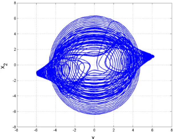
Fig. 1 depicts the strange attractor of the novel system (A) in 3-D view, while Figs. 2, 3 and 4 depict the 2-D projection of this system (A) in ( ,x x₁ ₂),

2 3 ( , )x x and

3 1

( , )x x plane, respectively.

Fig. 1. Strange chaotic attractor of the novel system (A).

(3)

Fig. 3. A 2-D projection of the novel system (A) in the (x₂,x₃)−plane.

Fig. 4. A 2-D projection of the novel system (A) in the (x3,x1)−plane.

The novel system (B) is defined by the 3-D dynamics:

! x

1=α(x2−x1)+x2x3

!

x

2=βx1−γx1x3 !

x

3=−δx3+cosh(x1x2)

(3)

where x x₁, ₂,x₃ are states and α β γ δ, , , are constant, positive, parameters of the system (3).

We note that the system (B) has a quadratic nonlinearity in each of the first two equations and a hyperbolic cosinusoidal nonlinearity in the last equation.

The system (3) exhibits a strange chaotic attractor for the parameter values

10, 98, 2, 10

= = = =

α β γ δ (4)

For numerical simulations, we have used classical fourth-order Runge-Kutta method (MATLAB) for solving the system (B) when the initial conditions are taken as

1(0)=0.4, (0)2 =−0.6, (0)3 =0.7

x x x

Fig. 5 depicts the strange attractor of the novel system (B) in 3-D view, while Figs. 6, 7 and 8 depict the 2-D projection of this system (B) in ( ,x x₁ ₂),

2 3

( , )x x and( , )x₃ x₁ plane, respectively.

Fig. 5. Strange chaotic attractor of the novel system (B).

Fig. 6. A 2-D projection of the novel system (B) in the ( ,x1x2)−plane.

Fig. 7. A 2-D projection of the novel system (B) in the (x2,x3)−plane.

(4)

3. Analysis of the Novel Chaotic System (A) with Hyperbolic Sinusoidal Nonlinearity

A. Symmetry and Invariance

We note that the novel chaotic system (A) is invariant under the coordinates transformation

1 2 3 1 2 3

( ,x x ,x)→ −( x,−x ,x).

Thus, the novel chaotic system (A) has rotation symmetry about the x3−axis.

B. Dissipativity

In vector notation, the novel chaotic system (A) can be expressed as

!

x= f (x)= f₁(x)

f₂(x)

f₃(x)

!

" # # # #

$

% & & & &

(3)

The divergence of the vector field f on 3

R is given by

1 2 3

( ) ( ) ( )

div( ) ∂ ∂ ∂

∇ ⋅ = = + +

∂ ∂ ∂

f x f x f x

f f

x x x (4)

The divergence of the vector field f measures the rate at which the volumes change under the flow Φtof f.

Let D be any given region in 3

R with a smooth boundary. Let D t( )=Φt( ).D Let V t( )denote the volume of

( ). D t

By Liouville’s theorem, we have

( ) ( )

( )

=

_∫

∇ ⋅

D t dV t

f dx dy dz

dt (5)

Using the equation (1) of the novel system (A), we find that

1 2 3

( ) 0

∂ ∂ ∂

∇ ⋅ = + + =− + <

∂ ∂ ∂

f f f

f a d

x x x (6)

since a and d are positive constants.

By substituting the value of ∇ ⋅f in Eq. (5), we get

( )

( ) ( ) ( )

=− +

∫

=− +

D t dV t

a d dx dy dz a d V t

dt (7)

Solving the linear ODE (7), we get the solution

(

)

( )= (0)exp −( + )

V t V a d t (8)

From Eq. (8), it follows that any volume V t( )_{must shrink} to zero exponentially as t→ ∞._{Thus, the novel chaotic} system (A) is a dissipative chaotic system.

Hence, the asymptotic motion of the novel system (A) settles onto a strange attractor of the novel system (A).

C. Equilibrium Points

We obtain the equilibrium points of the novel chaotic system

(A) by solving the nonlinear system of equations:

( )=0

f x (9)

Assume that a b c d, , , >0_anddb>c.

Solving the equations (9), we get three equilibrium points of the novel chaotic system (A), which are described as follows:

0

1

2 : (0,0,0)

: ln( ) , ln( ) ,

 + 

 

 ₊ 

 

 + 

− −

 

 ₊ 

 

E

ac b ac b

E m m

ac ac b c

ac b ac b

E m m

ac ac b c

where m=p+ ₁+p2 and _p₌db. c

We take the parameter values as in the chaotic case, viz.

10, 92, 2, 10.

= = = =

a b c d ₍₁₀₎

Then the three equilibrium points of the novel system (A) are obtained as

0

1

2 : (0,0,0)

: (6.1819, 1.1039, 46)

: ( 6.1819, 1.1039,46)− − E

E E

(11)

Using the first method of Lyapunov, it is easy to see that

0

E

is a saddle point and E E₁, ₂ are saddle-foci. Hence, all the equilibrium points of the novel system (A) are unstable.

D. Lyapunov Exponents We take the initial state as:

1(0) 0.4, (0) 1.0, (0) 0.6= 2 = 3 =

x x x (12)

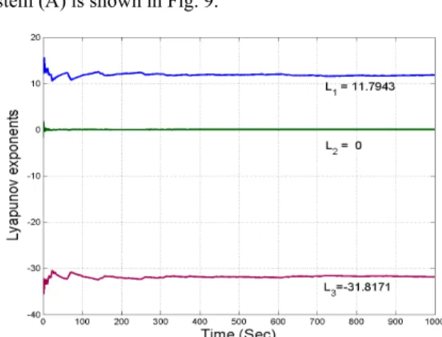
Also, we take the parameters as given in (10). Then the Lyapunov exponents of the novel chaotic system (A) are obtained numerically using MATLAB as

1=11.7943, 2=0, 3=−31.8171

L L L (13)

This shows mathematically that the novel system (A) is indeed chaotic. Note that the maximal Lyapunov exponent (MLE) of the novel system (A) is _L₁=11.7943, which is a large value. Thus, the novel system (A) depicts strong chaotic behaviour.

E. Kaplan-Yorke Dimension

The Kaplan-Yorke dimension of the system (A) is

1 2

1 ₁ 3

1

2 2.3707

| ₊ | | |

=

+

= +

∑

= + =

j

KY i

j _i

L L

D j L

L L (14)

Eq. (14) shows that the system (A) is a dissipative system and the Kaplan-Yorke dimension of the system (A) is fractional.

(5)

system (A) is shown in Fig. 9.

Fig. 9. Dynamics of the Lyapunov exponents of the novel system (A).

4. Analysis of the Novel Chaotic System (B) with Hyperbolic Cosinusoidal Nonlinearity

A. Symmetry and Invariance

We note that the novel chaotic system (B) is invariant under the coordinates transformation

1 2 3 1 2 3

( ,x x ,x)→ −( x,−x ,x).

Thus, the novel chaotic system (B) has rotation symmetry about the x3−axis.

B. Dissipativity

In vector notation, the novel chaotic system (B) can be expressed as

!

x= f (x)= f₁(x)

f₂(x)

f₃(x) !

" # # # #

$

% & & & &

(15)

The divergence of the vector field f on 3

R is given by

1 2 3

( ) ( ) ( )

div( ) ∂ ∂ ∂

∇ ⋅ = = + +

∂ ∂ ∂

f x f x f x

f f

x x x (16)

The divergence of the vector field f measures the rate at which the volumes change under the flow Φtof f.

Let D be any given region in 3

R with a smooth boundary. Let D t( )=Φt( ).D Let V t( ) denote the volume of V t( )

By Liouville’s theorem, we have

( ) ( )

( )

=

∫

∇ ⋅

D t dV t

f dx dy dz

dt (17)

Using the equation (3) of the novel system (B), we find that

1 2 3

( ) 0

∂ ∂ ∂

∇ ⋅ = + + =− + <

∂ ∂ ∂

f f f

f

x x x α δ (18)

since a and δ_{are positive constants.}

By substituting the value of ∇ ⋅f ∇ ⋅f in Eq. (18), we get:

( ) ( )

( ) ( ) ( )

=− +

∫

=− +

D t

dV t

dx dy dz V t

dt α δ α δ (19)

Solving the linear ODE (19), we get the solution:

(

)

( )= (0)exp −( + )

V t V

_{α δ}

t (20)

From Eq. (20), it follows that any volume V t( )_must shrink to zero exponentially as t_{→ ∞}._{Thus, the novel}

chaotic system (B) is a dissipative chaotic system.

Hence, the asymptotic motion of the novel system (B) settles onto a strange attractor of the novel system (B).

C. Equilibrium Points

We obtain the equilibrium points of the novel chaotic system (B) by solving the nonlinear system of equations

( )=0

f x (21)

Assume that α β γ δ, , , >0 and _δβ_>_γ.

Solving the equations (21), we get three equilibrium points of the novel chaotic system (B), which are described as follows:

0

1

2 : (0,0,0)

: ln( ) , ln( ) ,

 + 

 

 ₊ 

 

 + 

− −

 

 ₊ 

 

E

E n n

αγ β αγ β

αγ αγ β γ

αγ β αγ β

αγ αγ β γ

where n=q+ 1+q2 and _q₌δβ. γ

We take the parameter values as in the chaotic case, viz.

10, 98, 2, 10.

= = = =

α β γ δ (22)

Then the three equilibrium points of the novel system (B) are obtained as:

0

1

2 : (0,0,0)

: (6.3747, 1.0805, 49)

: ( 6.3747, 1.0805,49)− − E

E E

(23)

Using the first method of Lyapunov, it is easy to see that

0

E is a saddle point and E E₁, ₂are saddle-foci. Hence, all the equilibrium points of the novel system (B) are unstable.

D. Lyapunov Exponents We take the initial state as

1(0) 0.4, (0) 1.0, (0) 0.6= 2 = 3 =

x x x (24)

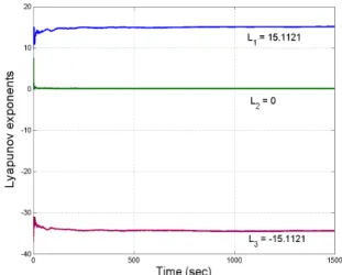
Also, we take the parameters as given in (22). Then the Lyapunov exponents of the novel chaotic system (B) are obtained numerically using MATLAB as:

1=15.1121, 2=0, 3=−34.4401

(6)

This shows mathematically that the novel system (B) is indeed chaotic. Note that the maximal Lyapunov exponent (MLE) of the novel system (B) is _L₁=15.1121, which is a large value. Thus, the novel system (B) depicts strong chaotic behaviour.

E. Kaplan-Yorke Dimension

The Kaplan-Yorke dimension of the system (B) is

1 2

1 ₁ 3

1

2 2.4388

| ₊ | | |

=

+

= +

∑

= + =

j

KY i

j _i

L L

D j L

L L (26)

Eq. (26) shows that the system (B) is a dissipative system and the Kaplan-Yorke dimension of the system (B) is fractional.

The dynamics of the Lyapunov exponents of the novel system (B) is shown in Fig. 10.

Fig. 10. Dynamics of the Lyapunov exponents of the novel system (B).

5. Adaptive Synchronization of the Novel Chaotic Systems (A) with Unknown Parameters

In this section, we shall discuss the adaptive synchronization of the novel chaotic systems (A) with unknown system parameters. Using adaptive control method, we design an adaptive synchronizer, which makes use of estimates of the unknown system parameters, and the error convergence is established for all initial conditions using Lyapunov stability theory [65].

As the master (or drive) system, we consider the novel system (A), which is described by

! x

1=a(x2−x1)+x2x3 !

x

2=bx1−cx1x3

!

x

3=−dx3+sinh(x1x2)

(27)

where x x₁, ₂,x₃ are the states and a b c d, , , _{are unknown} system parameters.

As the slave (or response) system, we consider the controlled novel system (A), which is described by

!

y₁=a(y₂−y₁)+y₂y₃+u₁

!

y₂=by₁−cy₁y₃+u₂

!

y₃=−dy₃+sinh(y₁y₂)+u₃

(28)

where y y y1, 2, 3are the states and u u1, 2,u3 are adaptive controllers to be designed.

We define the chaos synchronization error between the systems (27) and (28) as:

1 1 1

2 2 2

3 3 3

= −

e y x

(29)

The synchronization error dynamics is easily obtained as:

1 2 1 2 3 2 3 1

2 1 1 3 1 3 2

3 3 1 2 1 2 3

( )

sinh( ) sinh( )

= − + − +

= − − +

=− + − +

&

e a e e y y x x u

e be c y y x x u

e de y y x x u

(30)

Next, we introduce the nonlinear controller defined by

1 2 1 2 3 2 3 1 1

2 1 1 3 1 3 2 2

3 3 1 2 1 2 3 3

ˆ( )( )

ˆ_{( )} _ˆ_{( )(} ₎

ˆ( ) sinh( ) sinh( )

=− − − + −

=− + − −

= − + −

u a t e e y y x x k e

u b t e c t y y x x k e

u d t e y y x x k e

(31)

where a t b t c t d tˆ( ), ( ), ( ), ( )ˆ ˆ ˆ are estimates of the unknown

system parameters a b c d, , , _{respectively, and}

1, 2, 3 k k k are

positive gains. By substituting the control law (31) into (30), we get the closed-loop error dynamics as:

1 2 1 1 1

2 1 1 3 1 3 2 2

3 3 3 3

ˆ

( ( ))( )

ˆ _ˆ

( ( )) ( ( ))( )

ˆ ( ( ))

= − − −

= − − − − −

=− − −

&

e a a t e e k e

e b b t e c c t y y x x k e

e d d t e k e

(32)

We define the errors in estimating system parameters as

ˆ ( ) ( )

= −

a

b

c

d

e t a a t

e t b b t

e t c c t

e t d d t

(33)

Differentiating (33) with respect to t, we obtain

! e

a(t)=−ˆ ! a₍t₎

! e

b(t)=−ˆ !

b₍t₎

! e

c(t)=−ˆ

!

c₍t₎

! e

d(t)=−ˆ

!

d₍t₎

(34)

The error dynamics (32) can be simplified by using (33) as:

! e

1=ea(e2−e1)−k1e1 !

e₂=e_be₁−e_c(y₁y₃−x₁x₃)−k₂e₂ !

e

3=−ede3−k3e3

(7)

Next, we derive an update law for the parameter estimates using Lyapunov stability theory. So, we take a candidate Lyapunov function defined by

(

2 2 2 2 2 2 2

)

1 2 3

1

, 2

= + + + a+ b+ c+ d

V e e e e e e e (36)

which is a quadratic and positive-definite function on 7

.

R Next, we calculate the time-derivative of V along the trajectories of (34) and (35). We obtain

! V =−k

1e1 2₋_k

2e2 2₋_k

3e3 2₊_e

a e1(e2−e1)−ˆ

! a

"

# $%+eb e1e2−ˆ

!

b

" #&

$ %'

+e_c"−e₂(y₁y₃−x₁x₃)−cˆ!

# $%+ed −e3 2

−dˆ! " #&

$ %'

(37)

To guarantee global exponential stability of the systems (34) and (35), we need to choose parameter updates in such a way that V&_{is a quadratic, negative definite function on} 7

. R Thus, we choose the parameter update law as follows:

ˆ

!

a=e₁(e₂−e₁)+k₄e_a

ˆ !

b=e1e2+k5e_b

ˆ !

c=−e₂(y₁y₃−x₁x₃)+k₆e_c

ˆ ! d =−e3

2

+k7e_d

(38)

where k₄,k₅,k₆,k₇are positive constants. Next, we prove the main result of this section.

Theorem 1. The adaptive controller defined by (31) and the parameter update law defined by (38) globally and exponentially synchronize the novel chaotic systems (A) with unknown parameters described by the equations (27) and (28), where ki,(i=1,_K,7) are positive constants. The

parameter estimation errors ea( ), ( ), ( ),t e t e t eb c d( )t exponentially converge to zero with time.

Proof. The assertions are established using Lyapunov stability theory [65].

We have already noted that the Lyapunov function V defined by (36) is quadratic and positive definite on R7.

Next, we substitute the parameter update law defined by (38) into the dynamics (37). This simplifies the dynamics (37) as

!

V ₌₋k

1e1 2

−k

2e2 2

−k

3e3 2

−k

4ea

2 −k

5eb

2 −k

6ec

2 −k

7ed

2

(39)

which is a quadratic and negative definite function on R7. Hence, by Lyapunov stability theory [65], the synchronization and parameter estimation errors globally and exponentially converge to zero with time.

This completes the proof. !

For numerical simulations, the classical fourth order Runge-Kutta method with step size h₌10−8has been used with MATLAB to solve the chaotic systems (27) and (28) when the adaptive controller (31) and the parameter update law (38) are applied.

We take the positive gains ki as ki=5,(i=1,K,7).

The values of the system parameters for the systems (27) and (28) are taken as in the chaotic case, viz.

10, 92, 2, 10

= = = =

a b c d

The initial state of the master system (27) is taken as:

1(0) 1.2, (0) 3.6, (0) 5.4= 2 = 3 =

x x x

The initial state of the slave system (28) is taken as:

1(0)=4.3, (0) 1.7, (0)2 = 3 =2.6

y y y

The initial values of the parameter estimates are taken as:

ˆ ˆ

ˆ(0)=2.9, (0)=4.5, (0) 6.8, (0) 5.1ˆ = =

a b c d

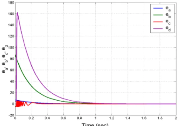
Fig. 11 depicts the complete chaos synchronization of the identical novel chaotic systems (A) described by the equations (27) and (28), while Fig. 12 depicts the time history of the synchronization errors e t₁( ), ( ), ( ).e₂ t e₃t Also, Fig. 13 depicts the time history of the parameter estimation errors

( ), ( ), ( ), ( ).

a b c d

e t e t e t e t

Fig. 11. Complete synchronization of the novel chaotic systems (A).

(8)

Fig. 13. Time history of the parameter estimation errors

( ), ( ), ( ), ( )

a b c d

e t e t e t e t _.

6. Adaptive Synchronization of the Novel Chaotic Systems (B) with Unknown Parameters

In this section, we shall discuss the adaptive synchronization of the novel chaotic systems (B) with unknown system parameters.

As the master (or drive) system, we consider the novel system (B), which is described by

!

x

1=α(x2−x1)+x2x3

!

x

2=βx1−γx1x3 !

x

3=−δx3+cosh(x1x2)

(40)

where x x₁, ₂,x₃ are the states and α β γ δ, , , are unknown system parameters. As the slave (or response) system, we consider the controlled novel system (B), which is described by

!

y₁=α(y₂−y₁)+y₂y₃+u₁

!

y₂=βy₁−γy₁y₃+u₂

!

y₃=−δy₃+cosh(y₁y₂)+u₃

(41)

where y y y₁, ₂, ₃ are the states and u u₁, ₂,u₃ are adaptive controllers to be designed. We define the chaos synchronization error between the systems (40) and (41) as:

1 1 1

2 2 2

3 3 3

= −

e y x

(42)

! e

1=α(e2−e1)+y2y3−x2x3+u1

!

e

2=βe1−γ(y1y3−x1x3)+u2

!

e

3=−δe3+cosh(y1y2)−cosh(x1x2)+u3

(43)

1 2 1 2 3 2 3 1 1

2 1 1 3 1 3 2 2

3 3 1 2 1 2 3 3

ˆ ( )( )

ˆ_{( )} _ˆ_{( )(} ₎

ˆ( ) cosh( ) cosh( )

=− − − + −

=− + − −

= − + −

u t e e y y x x k e

u t e t y y x x k e

u t e y y x x k e

α

β γ

δ

(44)

where

_α

ˆ( ), ( ), ( ), ( )t

_β

ˆ t

_γ

ˆt

_δ

ˆt are estimates of the unknown

system parameters α β γ δ, , , respectively, and k k₁, ₂,k₃ are positive gains.

By substituting the control law (44) into (43), we get the closed-loop error dynamics as:

! e

1=(α−αˆ(t))(e2−e1)−k1e1 !

e

2=(β−βˆ(t))e1−(γ−γˆ(t))(y1y3−x1x3)−k2e2

!

e

3=−(δ−δˆ(t))e3−k3e3

(45)

We define the errors in estimating system parameters as:

ˆ ( ) ( ) ˆ ( ) ( ) ˆ ( ) ( ) ˆ ( ) ( ) = − = − = − = −

e t t

α β γ δ α α β β γ γ δ δ (46)

! e

α(t)=−ˆ

! α(t₎

!

e

β(t)=−ˆ

! β(t₎

!

e

γ(t)=−ˆ

! γ(t₎

!

e

δ(t)=−ˆ ! δ(t₎

(47)

!

e

1=eα(e2−e1)−k1e1

! e

2=eβe1−eγ(y1y3−x1x3)−k2e2

! e

3=−eδe3−k3e3

(48)

(

2 2 2 2 2 2 2

)

1 2 3

1

, 2

= + + + + + +

V e e e e_α e_β e_γ e_δ (49)

which is a quadratic and positive-definite function on R7. Next, we calculate the time-derivative of V along the trajectories of (47) and (48). We obtain

! V =−k

1e1 2₋_k

2e2 2₋_k

3e3 2₊_e

α e1(e2−e1)−ˆ ! α

"

# $%+eβ e1e2− ˆ ! β " #& $ %' +e

γ −e2(y1y3−x1x3)−ˆ !

γ

"

# $%+eδ −e3

2₋_δˆ!

" #&

$ %'

(50)

(9)

ˆ ! α=e

1(e2−e1)+k4eα

ˆ

! β=e

1e2+k5eβ

ˆ ! γ=−e

2(y1y3−x₁x3)+k6eγ

ˆ

!

δ=−e

3 2

+k 7eδ

(51)

where k₄,k₅,k₆,k₇are positive constants. Next, we prove the main result of this section.

Theorem 2. The adaptive controller defined by (44) and the parameter update law defined by (51) globally and exponentially synchronize the novel chaotic systems (B) with unknown parameters described by the equations (40) and (41), where ki,(i=1,K,7) are positive constants. The

parameter estimation errors e ( ),t e ( ),t e ( ),t e ( )t

α β γ δ

exponentially converge to zero with time.

We have already noted that the Lyapunov function

Vdefined by (49) is quadratic and positive definite on R7.

Next, we substitute the parameter update law defined by (51) into the dynamics (50). This simplifies the dynamics (50) as

! V ₌₋k

1e1 2

−k 2e2

2

−k 3e3

2

−k 4eα

2

−k 5eβ

2

−k

6eγ 2

−k 7eδ

2

(52)

For numerical simulations, the classical fourth order Runge-Kutta method with step size h₌10−8 has been used with MATLAB to solve the chaotic systems (40) and (41) when the adaptive controller (44) and the parameter update law (51) are applied.

We take the positive gains kias ki=5,(i=1,K,7). The values of the system parameters for the systems (40) and (41) are taken as in the chaotic case, viz.

10, 98, 2, 10

= = = =

α β γ δ

10, 98, 2, 10

α= β= γ = δ =

1(0) 1.3, (0)= 2 =2.9, (0) 0.83 =

x x x

1(0)=2.1, (0) 1.7, (0) 5.32 = 3 =

y y y

ˆ ˆ

ˆ(0) 1.6, (0) 5.3, (0) 8.2, (0) 7.4= = ˆ = =

α

β

γ

δ

Fig. 14 depicts the complete chaos synchronization of the identical novel chaotic systems (B) described by the equations (40) and (41), while Fig. 15 depicts the time history of the synchronization errors e t₁( ), ( ), ( ).e₂ t e₃t Also, Fig. 16 depicts the time history of the parameter estimation errors

( ), ( ), ( ), ( ).

e t e t e t e t

α β γ δ

Fig. 14. Complete synchronization of the novel chaotic systems (B).

Fig. 15. Time history of the synchronization errors e t₁( ), ( ), ( )e₂ t e₃t .

( ), ( ), ( ), ( )

(10)

7. Adaptive Synchronization of the Novel Chaotic Systems (A) and (B) with Unknown Parameters

In this section, we shall discuss the adaptive synchronization of the novel chaotic systems (A) and (B) with unknown system parameters.

As the master (or drive) system, we consider the novel system (A), which is described by

! x

1=a(x2−x1)+x2x3

!

x

2=bx1−cx1x3

! x

3=−dx3+sinh(x1x2)

(53)

where x x1, 2,x3 are the states and a b c d, , , are unknown

system parameters. As the slave (or response) system, we consider the controlled novel system (B), which is described by

!

y₁=α(y₂−y₁)+y₂y₃+u₁

!

y₂=βy₁−γy₁y₃+u₂

!

y₃=−δy₃+cosh(y₁y₂)+u₃

(54)

wherey y y1, 2, 3 are the states, α β γ δ, , , are unknown system

parameters, and u u₁, ₂,u₃ are adaptive controllers to be designed. We define the chaos synchronization error between the systems (53) and (54) as:

1 1 1

2 2 2

3 3 3

= −

e y x

(55)

! e

1=α(y2−y1)−a(x2−x1)+y2y3−x2x3+u1

!

e

2=βy1−bx1−γy1y3+cx1x3+u2 !

e

3=−δy3+dx3+cosh(y1y2)−sinh(x1x2)+u3

(56)

1 2 1 2 1 2 3 2 3 1 1

2 1 1 1 3 1 3 2 2

3 3 3 1 2 1 2 3 3

ˆ( )( ) ˆ( )( ) ˆ

ˆ( ) ( ) ˆ( ) ˆ( )

ˆ

ˆ( ) ( ) cosh( ) sinh( )

u t y y a t x x y y x x k e

u t y b t x t y y c t x x k e

u t y d t x y y x x k e

α β γ δ = − − − − + − =− + + − − = − − + − (57)

where a tˆ( ),b tˆ( ),c tˆ( ),d tˆ( ),_αˆ ( ),t _βˆ( ),t

_γ

ˆ( ),t

δ

ˆ( )t are estimates of the unknown system parameters

,

a b, c,d,α,β,γ,δ,respectively, and k k₁, ₂,k₃ are

positive gains.

By substituting the control law (57) into (56), we get the closed-loop error dynamics as:

!

e

1=(α−α(tˆ ))(y2−y1)−(a−aˆ(t))(x2−x1)−k1e1

!

e

2=(β−β(ˆt))y1−(b−bˆ(t))x1−(γ−γ(tˆ ))y1y3+(c−c(tˆ ))x1x3−k2e2

! e

3=−(δ−δˆ(t))y3+(d−dˆ(t))x3−k3e3

(

58)

We define the errors in estimating system parameters as:

ˆ ˆ ˆ ˆ ( ) ( ), ( ) ( ), ( ) ( ), ( ) ( ) ˆ ˆ ˆ ˆ ( ) ( ), ( ) ( ), ( ) ( ), ( ) ( ) = − = − = − = − = − = − = − = −

a b c d

e t a a t e t b b t e t c c t e t d d t

e_αt α αt e_β t β βt e_γ t γ γ t e_δ t δ δt (59)

! e

a(t)=−ˆ

!

a(t), e!_b(t)=−bˆ!(t), e!

c(t)=−ˆ !

c(t), e!_d(t)=−dˆ!(t)

!

e

α(t)=−ˆ

! α(t), e!

β(t)=−ˆ !

β(t), e! γ(t)=−ˆ

! γ(t), e!

δ(t)=−ˆ ! δ(t) (60)

! e

1=eα(y2−y1)−ea(x2−x1)−k1e1 !

e

2=eβy1−ebx1−eγy1y3+ecx1x3−k2e2

!

e

3=−eδy3+edx3−k3e3

(61)

(

2 2 2 2 2 2 2 2 2 2 2

)

1 2 3

1

2

= + + + a+ b+ c+ d+ + + +

V e e e e e e e e e e e

α β γ δ (62)

which is a quadratic and positive-definite function on R11. Next, we calculate the time-derivative of V along the trajectories of (60) and (61). We obtain

!

V ₌₋k

1e1 2

−k 2e2

2

−k 3e3

2

+e

a −e1(x2−x1)−ˆ

! a "

# $%+eb −e2x1− ˆ

! b " #& $ %' +e

c e2x1x3−ˆ ! c

"

# $%+ed e3x3− ˆ

! d " #&

$

%'+eα e1(y2−y1)−ˆ !

α "

# $%

+e

β e2y1−ˆ

!

β

" #&

$

%'+eγ −e2y1y3−ˆ

! γ "

# $%+eδ −e3y3−ˆ

! δ " #& $ %' (63)

To guarantee global exponential stability of the systems (60) and (61), we need to choose parameter updates in such a way

that V&is a quadratic, negative definite function on R11. Thus, we choose the parameter update law as follows:

ˆ

!

a₌₋e

1(x2−x1)+k4ea ˆ

!

b₌₋e

2x1+k5eb ˆ

!

c₌e

2x1x3+k6ec ˆ

! d ₌e

3x3+k7ed ˆ

! α=e

1(y2−y1)+k8eα ˆ

! β=e

2y1+k9eβ ˆ

!

γ=−e

2y1y3+k10eγ ˆ

!

δ=−e

3y3+k11eδ

(64)

where ki,(i=4,K,11) are positive constants. Next, we prove the main result of this section.

(11)

and (54), where ki,(i=1,_K,11)are positive constants. All the parameter estimation errors exponentially converge to zero with time.

We have already noted that the Lyapunov function

V defined by (62) is quadratic and positive definite on R7. Next, we substitute the parameter update law defined by (64) into the dynamics (63). This simplifies the dynamics (63) as:

! V ₌₋k

1e1 2

−k 2e2

2

−k 3e3

2

−k 4ea

2

−k 5eb

2

−

₋k 6ec

2

−k 7ed

2

−k 8eα

2

−k 9eβ

2

−k 10eγ

2

−k

11eδ

2 (65)

For numerical simulations, the classical fourth order

Runge-Kutta method with step size h₌10−8 has been used with MATLAB to solve the chaotic systems (53) and (54) when the adaptive controller (57) and the parameter update law (64) are applied. We take the positive gains ki as

5,( 1, ,11). = = K

i

k i

The values of the system parameters for the systems (53) and (54) are taken as in the chaotic case, viz.

10, 92, 2, 10, 10, 98, 2, 10

= = = = = = = =

a b c d _α _β _γ _δ

1(0) 0.8, (0)= 2 =2.1, (0) 1.73 =

x x x

1(0)=2.4, (0)2 =0.2, (0) 3.53 =

y y y

ˆ ˆ

ˆ(0) 3.8, (0) 4.1, (0)ˆ 6.7, (0) 5.6,

ˆ ˆ

ˆ(0) 2.4, (0) 3.8, (0)ˆ 5.4, (0) 6.2

= = = =

a b c d

α β γ δ

Fig. 17 depicts the complete chaos synchronization of the identical novel chaotic systems (A) and (B), which are described by the equations (53) and (54) respectively, while Fig. 18 depicts the time history of the synchronization errors

1( ), ( ), ( ).2 3

e t e t e t Also, Fig. 19 depicts the time history of the

parameter estimation errors ea( ), ( ), ( ),t e t e t eb c d( ).t Finally, Fig. 20 depicts the time history of the parameter estimation errors e_α( ),t e_β( ),t e_γ( ),t e_δ( ).t

Fig. 17. Complete synchronization of the novel chaotic systems (A) and (B).

Fig. 18. Time history of the synchronization errors e t₁( ), ( ), ( )e₂ t e₃t .

( ), ( ), ( ), ( )

a b c d

(12)

( ), ( ), ( ), ( )

e t e t e t e t

α β γ δ .

8. Conclusion

In this research work, we have derived two novel 3-dimensional chaotic systems, the first with a hyperbolic sinusoidal nonlinearity and two quadratic nonlinearities (denoted as system (A)) and the second with a hyperbolic cosinusoidal nonlinearity and two quadratic nonlinearities (denoted as system (B)). First, we provided a detailed qualitative analysis of the two novel chaotic systems (A) and (B). We also calculated the Lyapunov exponents and Kaplan-Yorke dimensions of the chaotic systems (A) and (B). It was found that the maximal Lyapunov exponent (MLE) for the novel chaotic systems (A) and (B) has a large value, viz.

1=11.7943

L for system (A) and L1=15.1121for system (B). Using the Lyapunov stability theory, we have also derived adaptive controllers for synchronizing identical chaotic systems (A), identical chaotic systems (B) and non-identical chaotic systems (A) and (B). MATLAB plots were shown to illustrate the adaptive controller design numerically for the synchronization of the novel chaotic systems (A) and (B).

______________________________ References

1. E.N. Lorenz, J. Atmospheric Sci. 20, 130 (1963). 2. O.E. Rössler, Phy. Lett. 57A, 397 (1976).

3. M.I. Rabinovich, and A.L. Fabrikant, Sov. Phys. JETP. 50, 311 (1979).

4. A. Arneodo, P. Coullet, and C. Tresser, Phys. Lett. A. 79, 259 (1980).

5. T. Shimizu, and N. Morioka, Phy. Lett. A. 76, 201 (1980). 6. M.P. Kennedy, IEEE Trans. Circuits Sys. 41, 771 (1994). 7. R. Shaw, Zeitschrift für Natur. 36, 80 (1981).

8. L.O. Chua, T. Matsumoto, and M. Komuro, IEEE Trans. Circuits Sys. 32, 798 (1985).

9. A.M. Rucklidge, J. Fluid Mech. 237, 209 (1992). 10. J.C. Sprott, Phys. Rev. E, 50, 647 (1994).

11. G. Chen, and T. Ueta, Internat. J. Bifur. Chaos. 9, 1465 (1999). 12. J. Lü, and G. Chen, Internat. J. Bifur. Chaos. 12, 659 (2002). 13. H.K. Chen, and C.I. Lee, Chaos, Solit. Fract. 21, 957 (2004). 14. G. Tigan, and D. Opris, Chaos, Solit. Fract. 36, 1315 (2008). 15. G. Cai, and Z. Tan, J. Uncertain Sys. 1, 235 (2007). 16. D. Li, Phy. Lett. A. 372, 387 (2008).

17. L. Wang, Nonlinear Dyn. 56, 453 (2009).

18. A.M. Harb, B.A. Harb, Chaos, Solit. Fract. 20, 719 (2004). 19. V. Sundarapandian, and I. Pehlivan, Math. Computer Modelling.

55, 1904 (2012).

20. C. Gissinger, Euro. Phys. J. B. 85, 3667 (2012).

21. Z. Wei, and Q. Yang, Nonlinear Analysis: RWA. 12, 106 (2011).

22. F. Yu, and C. Wang, Eng. Tech. Appl. Sci. Res. 2, 209 (2012). 23. F. Yu, C. Wang, Q. Wan, and Y. Hu, Pramana. 80, 223 (2013). 24. F. Yu, and C. Wang, ETASR. 3, 352 (2013).

25. F. Saif, Phy. Reports. 419, 207 (2005).

26. S.V. Prants, Comm. Nonlinear Sci. Num. Simul. 17, 2713 (2012).

27. E.M. Shahverdiev, and K.A. Shore, Chaos, Solit. Fract. 38, 1298 (2008).

28. J.F. Liao, and J.Q. Sun, Optics Commun. 295, 188 (2013). 29. A. Shabunin, V. Astakhov, V. Demidov, A. Provata, F. Baras,

G. Nicolis, and V. Anishchenko, Chaos, Solit. Fract. 15, 395 (2003).

30. Q.S. Li, and R. Zhu, Chaos, Solit. Fract. 19, 195 (2004). 31. R. Engbert, and F.R. Drepper, Chaos, Solit. Fract. 4, 1147

(1994).

32. I. Suárez, Ecology. 117, 305 (1999). 33. T.R. Chay, Physica D. 16, 233 (1985).

34. A. Munteanu and R.V. Solé, J. Theor. Biology. 240, 434 (2006). 35. H. Cheng, and A. Sandu, Env. Model. Soft. 24, 917 (2009). 36. H. Yuxia, and Z. Hongtao, Physics Procedia. 25, 588 (2012). 37. U. Nechmzow, and K. Walker, Robo. Auto. Sys. 53, 177 (2005).

38. B.H. Kaygisiz, I. Erkmen, and A.M. Erkmen, Chaos, Solit. Fract. 29, 148 (2006).

39. J. Zhou, H.B. Huang, G.X. Qi, P. Yang, and X. Xie, Phy. Lett. A. 335, 191 (2005).

40. G. Kaddoum, M. Coulon, D. Roviras, and P. Chargé, Signal Processing. 90, 2923 (2010).

41. M. Usama, M.K. Khan, K. Algathbar, and C. Lee, Comp. Math. Appl. 60, 326 (2010).

42. H. Hermassi, R. Rhouma, and S. Belghith, J. Sys. Soft. 85, 2133 (2012).

43. G. He, Z. Cao, P. Zhu, and H. Ogura, Neural Networks. 16, 1195 (2003).

44. E. Kaslik, and S. Sivasundaram, Neural Networks, 32, 245 (2012).

45. D. Guégan, Annual Rev. Control. 33, 89 (2009).

46. L.M. Pecora, and T.L. Carroll, Phys. Rev. Lett. 64, 821 (1990). 47. V. Sundarapandian, Internat. J. Computer Info. Sys. 2, 6 (2011). 48. P. Sarasu, and S. Vaidyanathan, Internat. J. Systems Signal

Control Eng. Appl. 4, 26 (2011).

49. S. Vaidyanathan, and K. Rajagopal, Internat. J. Systems Signal Control Eng. Appl. 4, 55 (2011).

50. V. Sundarapandian, and R. Karthikeyan, J. Eng. Appl. Sci. 7, 254 (2012).

51. V. Sundarapandian, and R. Karthikeyan, Euro. J. Scientific Research. 64, 94 (2011).

52. S. Vaidyanathan, and K. Rajagopal, Internat. J. Soft Comput. 7, 28 (2012).

53. P. Sarasu, and V. Sundarapandian, Internat. J. Soft Comput. 7, 146 (2012).

54. S. Vaidyanathan, Internat. J. Control Theory Appl. 5, 45 (2012). 55. J.J. Yan, M.L. Hung, T.Y. Chiang, and Y.S. Yang, Phy. Lett. A.

356, 220 (2006).

56. J.J. Yan, J.S. Lin, and T.L. Liao, Chaos, Solit. Fract. 36, 45 (2008).

57. V. Sundarapandian, and S. Sivaperumal, Internat. J. Soft Comput. 6, 224 (2011).

58. S. Vaidyanathan, and S. Sampath, Internat. J. Automat. Comput.

9, 274 (2012).

59. C. Wang, and S.S. Gu, Chaos, Solit. Fract. 12, 1199 (2001). 60. U.E. Vincent, A. Ucar, J.A. Laoye, and S.O. Kareem, Physica C:

Superconduct. 468, 374 (2008).

61. S. Rasappan, and S. Vaidyanathan, Archi. Control Sci. 22, 343 (2012).

62. R. Suresh, and V. Sundarapandian, Far East J. Math. Sci. 73, 73 (2013).

(13)

64. T.H. Lee, Z.G. Wu, and J.H. Park, Applied Math. Comput. 219, 1354 (2012).