A Fast DOA Estimation Algorithm Based on Polarization MUSIC

A Fast DOA Estimation Algorithm Based

on Polarization MUSIC

Ran GUO

, Xing-Peng MAO

, Shao-Bin LI

, Yi-Ming WANG

, Xiu-Hong WANG

1_{School of Electronic and Information Engineering, Harbin Institute of Technology, Harbin, Heilongjiang Province, China} 2_{The First Institute of Oceanography, SOA, Qingdao, Shandong Province, China}

mxp@hit.edu.cn

Abstract. A fast DOA estimation algorithm developed from MUSIC, which also benefits from the processing of the signals’ polarization information, is presented. Besides performance enhancement in precision and resolution, the proposed algorithm can be exerted on various forms of polarization sensitive arrays, without specific requirement on the array’s pattern. Depending on the continuity property of the space spectrum, a huge amount of computation incurred in the calculation of 4-D space spectrum is averted. Performance and computation complexity analysis of the proposed algorithm is discussed and the simulation results are presented. Compared with conventional MUSIC, the proposed algorithm has considerable advantage in aspects of precision and resolution, with a low computation complexity proportional to a conventional 2-D MUSIC.

Keywords

Polarization sensitive array, DOA, MUSIC, fast algo-rithm.

1. Introduction

The direction of arriving signals (DOA) estimation problem has raised great interest in various fields, including radar, mobile communications, and microphone array systems. In the past decades, numerous algorithms and techniques have been proposed. Some important classes of algorithms include the Maximum Likelihood Estimation (ML) [1, 2], the signal subspace based algorithms rep-resented by Multiple Signal Classification (MUSIC) [3], and the computationally efficient Estimation of Signal Parameters via Rotational Invariance Techniques (ESPRIT) [4]. These algorithms help to enhance the performance of the DOA estimation substantially, and a great number of relevant algorithms are derived from them, for instance, Stochastic Maximum Likelihood Estimation (SML) [5], Root-MUSIC [6], Total Least Squares version of ESPRIT (TLS-ESPRIT) [7], etc.. In recent years, sparse signal presentation has been introduced into DOA estimation [8, 9, 10], making the DOA estimation with small number of snapshots possible.

Of all these algorithms, ML and its derivate algorithms are of the best performance in both accuracy and resolution, whereas the computation complexity is extremely high, preventing their practical applications. ESPRIT and MUSIC algorithms, proposed later, with precision error approaches to the Cramer-Rao bound (CRB) as snapshot number of array outputs accumulates to a certain threshold, and the calculation incurred in these 2 algorithms are acceptable.

Numerous factors should be considered to select a proper algorithm. First, the DOA algorithm should adapt to the form of the array. Generally, the signals’ azimuths need to be estimated, and in certain circumstance, their elevation estimation are also demanded. Well-designed planar arrays, such as uniform circular array (UCA), can meet these requirements. However, ESPRIT and Root-MUSIC can only work on linear array, and algorithms derived from them for other array forms [11, 12, 13] can only work on particular array patterns, while only 1 direction parameter can be estimated. The MUSIC algorithm, which can be transplanted to more general forms of planar arrays and provides both azimuth and elevation estimation, seems to be more suitable. Current calculation capacity of DSP chips makes it practical as well.

For algorithm selection, another crucial factor is the performance, especially in aspects of precision and resolution. The results presented in [14, 15] suggested that the accuracy and resolution in MUSIC are both determined by three factors: SNR, the number of array’s snapshots, and the array’s aperture. In practical circumstances, the SNR is generally uncontrollable, the aperture is often restricted, and the numbers of samples is limited. From this perspective, the accuracy and resolution of MUSIC algorithm is confined, and further improvement in performance can only be sought within other methods.

The polarization phenomenon of electromagnetic wave has been noticed and studied by physicists for more than a century. However, it was only in 1980s that this phenomenon began to attract the researchers’ attention and proved to be of great advantage in signal processing. The polarization sensitive array is introduced into DOA estimation by Nehorai and Li [16, 17]. In [17, 18], Jian Li integrated the polarization into ESPRIT successfully. The pencil-MUSIC algorithm is devised for DOA and

polarization estimation in [19, 20, 21], which extend the ESPRIT-like algorithm to partially polarized sources. [22, 23] provide an algorithm based on sparse ULA, consisting of sensors which can measure all six electrical and magnetic components. [24] provide several algorithms to solve the correlation problem with the array of vector sensors. In [25, 26], the polynomial rooting algorithm was adopted in polarization sensitive arrays. Covariance tensor [27, 28] is introduced to define the array manifold in a new way and reduce the amount of calculation. These papers exploited the advantage of polarization of signals. However, to reduce the calculation complexity, all these algorithms assumed specific patterns of array, and most of them adopted the sensors with the capacity to detect all 6 electrical and magnetic components, which is not very applicable.

The algorithms presented in [29-33] require no assistance of magnetic components. But the algorithms mentioned in [29, 30] assumed that 1 polarization parameter and 1 direction parameter are predetermined, which cannot be satisfied generally. In [31, 32, 33], the amount of calculation is reduced by dividing the process of estimation into two steps: one concerns with the polarization, and the other with the direction. The drawback of this method is that the second step in the algorithm depends on the success of previous step. When the DOAs of multiple signals are very close, the second step inclines to fail, even when the signals are distinct in polarization domain.

To retain the advantage in resolving close signals offered combination of spatial and polarization domains, a new algorithm, which reveals the space-polarization spectrum of 4-D space in a new way, is proposed in this paper. Unlike the algorithms mentioned above, the proposed algorithm can be used on various forms of polarization sensitive arrays. Besides, in case the multiple signals are close in space domain, they can be resolved as they are distinctive in polarization domain. By analyzing the property of the space spectrum, the algorithm is designed to reduce the complexity of the 4-D space spectrum calculation to be proportional to a 2-D spectrum calculation [34]. The proposed algorithm makes the transplantation of MUSIC from arrays of ideal omnidirectional antennas to polarization sensitive arrays more practical.

This paper is organized as follows. In Sec. 2, the fundamental principle of MUSIC is introduced, and the transplantation of MUSIC into polarization sensitive array is discussed. Although the latter one is highly inapplicable because of the immense amount of calculation, it is essential in developing the faster new algorithm. In Sec. 3, the definition of zero spectrum and another form of space spectrum are given, and the continuous and differential properties of them are studied. Based on these properties, calculation complexity in the 2-D peaks searching of polarization domain can be reduced dramatically. In Sec. 4, the analysis on the accuracy and resolution performance is presented, and the analysis of algorithm complexity is

discussed as well. In Sec. 5, simulation results are provided to demonstrate the continuous property mentioned in Sec. 3, and the accuracy and resolution performance.

2. MUSIC’s Transplantation into

Polarization Sensitive Array

2.1 Principle of Conventional MUSIC

Consider an arbitrary array (not a polarization sensitive array) which consists of M elements, and N narrow-band zero-mean signals of the same central frequency, arriving at the array from different directions. It is assumed that these signals are uncorrelated with each other, andM>N. The output of theith element can be written as:

xi(t) = N

∑

k=1

sk(t)exp(−jω0τki) +ni(t) (1)

where sk(t) is the kth signal, ni(t) is the Additive White

Gaussian Noise (AWGN), andω0 is the central frequency of all the N signals. The parameter τki is the delayed

time of the kth signal at the ith element, whose form is determined by the direction of impinging signals and the pattern of the array. For a ULA, τki is (i−1)dsinϕk/c,

whereϕk represents the azimuth of thekth signal, d is the

element spacing andcis the propagation velocity of signals; for a UCA withM elements, τki becomesrsinθkcos(ϕk−

2πi/M)/c, whereθk andϕk are the elevation and azimuth

of the kth signal respectively, and r represents the radius of the UCA. For general planar arrays, the time elpase τki

becomes(xisinθkcosϕk+yisinθksinϕk)/c, wherexiandyi

are used to indicate the location of theith element. Using vector forms, (1) can be written as:

X(t) =AS(t) +N(t) (2) where the output vector is X(t) = [x1(t), . . . ,xM(t)]T, the

signal vector is S(t) = [s1(t), . . . ,sN(t)]T, and the noise

vector isN(t) = [n1(t), . . . ,nM(t)]T;Ais the matrix of array

manifold, and the element on its kth row and ith column is [A]ki=exp(−jω0τki). The operator (∗)T indicates the

transposed matrix.

Then the covariance matrix ofX(t)is: Rx=E[X(t)XH(t)]

=ARSAH+σ2NI

=

M

∑

i=1

λiuiuHi

(3)

whereλirepresents the eigenvalue ofRX, arranged asλ1>

λ2>···>λN+1=···=λM=σ2N.σ2N is the power of white

noise, anduidenotes the eigenvector corresponding toλi.I

is the identity matrix. From (3) we have:

ARSAH=

N

∑

i=1

Equation (4) indicates the fact that the column vectors of the matrix A, which are also referred as steering vectors, are within the N-dimension space spanned by the first N eigenvectors, perpendicular to the noise subspace spanned by the otherM₋Neigenvectors.

In MUSIC algorithm [3], the form space spectrum is defined as:

P= 1

∑Mi=N+1aHui

= 1

kaH_U Nk2

(5)

where the operator k∗k denotes the Euclidean norm, and U_N= [u_N+1,uN+2, . . . ,uM], whose column vectors span the

noise subspace. Corresponding to the signal subspace, US= [u1,u2, . . . ,uN]. The form of vector a is similar to

that of the column vectors ofA. Every component of ais a function of the 2 direction parameters : the azimuth ϕ

and elevationθ. The space spectrumP can be considered as a function of them as well. By calculating the spectrum in the space domain and searching the values of the parameters corresponding to theN maxima ofP, the directions of the arriving signals can be estimated. The amount of calculation incurred in this process depends on the number of parameters determining the signal’s direction. For ULA, all signals are assumed to be within a planar, and a 1-D search within the range of azimuth ϕcan estimate their directions; whereas for a UCA or a planar array, a 2-D search on the azimuth

ϕand elevationθis required, and the amount of calculation increases considerably.

2.2 Polarization MUSIC

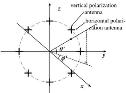
Consider a UCA ofMpolarized sensitive elements (as shown in Fig. 1, whereM=8). AssumingNsignals arrive at the array, as mentioned in [17, 18], theith column vector ofAin (2) becomes:

a(θi,ϕi,γi,ηi) =aS(θi,ϕi)⊗aP(θi,ϕi,γi,ηi) (6)

z

y

x θ'

φ'

vertical polarization antenna horizontal

polari-zation antenna

Fig. 1.An example of polarization sensitive array.

where ⊗ represents the Kronecker product, γi and ηi are

the polarization parameters of ith signal, and aS(θi,ϕi) is

the steering vector of theith signal on behalf of its spatial direction, written as:

aS(θi,ϕi) =

q0 q1 q2··· qM−1 T

. (7)

In a UCA theqkis:

qk=exp

2πr

λ sinθicos

ϕi−

2πk M

. (8)

The vector aP(θi,ϕi,γi,ηi) which represents the effect of

polarization is:

aP(θi,ϕi,γi,ηi)

=

cosθicosϕi −sinϕi

cosθisinϕi cosϕi

sinγiejηi

cosγi

_{. (9)}

Substitute (6) into (2), following the similar program in [29] we can define a new joint space spectrumPJ:

PJ(θ,ϕ,γ,η) =

1 kaH_{(θ,ϕ,γ,η)U}

Nk2

. (10)

Comparing (10) with (5), the only difference is that the space spectrumPJ becomes a function of 4 parameters: θ,

ϕ,γ andη, specifying the elevation angle, azimuth angle, and the 2 polarization parameters respectively. It should be noticed that, even if polarization states of all arriving signals are the same, as the direction parametersθiandϕiare

involved in vectoraP(θi,ϕi,γi,ηi), it still brings difference

into the steering vectora(θi,ϕi,γi,ηi)and helps to enhance

the algorithm’s resolution performance. However, when the combination of these 4 parameters makesaP(θi,ϕi,γi,ηi) =

aP(θj,ϕj,γj,ηj), i6= j, the polarization states no longer

provide assistance in resolving these 2 signals.

Theoretically, a peak search can be executed in a 4-D space spanned by these 4 parameters to obtain the estimation results. Benjamin Friedlander has proved that the performance of resolution will be improved considerably [35]. However, the calculation complexity of the 4-D space spectrum causes an unbearable computation complexity and makes the ordinary polarization MUSIC algorithm unpractical.

3. Fast Polarization MUSIC

In this part, properties of the space spectrum PJ(θ,ϕ,γ,η) of the polarization MUSIC is analyzed, and

a more effective algorithm is developed to reduce the great amount of calculation in DOA estimation.

3.1 Property of the Joint Space Spectrum

As previously stated, the values of the 4 parameters corresponding to the N maximums of the space spectrum in (10) indicate the directions and polarization states of the Narriving signals. And a maximum in 4-D space spanned by the 4 parameters, whose position is(θ0,ϕ0,γ0,η0), remains to be a maximum in the 2-D subspace(θ0,ϕ0,γ,η), spanned by the two polarization parameters.

a(θ0,ϕ0,γ,η)

=aS(θ0,ϕ0)⊗aP(θ0,ϕ0,γ,η)

=      q0 q1 .. . qM₋1

     ⊗

cosθ0cosϕ0sinγejη−sinϕ₀cosγ

cosθ0sinϕ0sinγejη+cosϕ₀cosγ

=     

u1(θ0,ϕ0)sinγejη+v1(θ₀,ϕ₀)cosγ

u2(θ0,ϕ0)sinγejη+v₂(θ₀,ϕ₀)cosγ

.. .

u2M(θ0,ϕ0)sinγejη+v_2M(θ₀,ϕ₀)cosγ

     (11) where:

u2k−1(θ0,ϕ0) =qk−1cosθ0cosϕ0 (12a) v2k−1(θ0,ϕ0) =−qk−1sinϕ0 (12b) u2k(θ0,ϕ0) =qk₋1cosθ0sinϕ0 (12c) v2k(θ0,ϕ0) =qk−1cosϕ0 (12d)

andk=1,2, . . . ,M.

As mentioned in [36], another form of the joint space spectrum in (10) can be derived:

PJ(θ,ϕ,γ,η) =Z−1(θ,ϕ,γ,η)

= [M₋U(θ,ϕ,γ,η)]−1 (13)

where:

Z(θ,ϕ,γ,η)

=kaH(θ,ϕ,γ,η)UNk2

=ka(θ,ϕ,γ,η)k2_{− ka}H_{(θ,ϕ,γ,η)U} Sk2

=M₋Msin2θsin2γ− kaH(θ,ϕ,γ,η)USk2

(14)

and:

U(θ,ϕ,γ,η) =Msin2θsin2γ+kaH(θ,ϕ,γ,η)USk2 (15)

where Z(θ,ϕ,γ,η) is named as zero spectrum, as it approaches to 0 when values of the 4 parameters approach to the direction and polarization state of a signal. At the same time,U(θ,ϕ,γ,η)in (13) approaches to a local maximum, and a steep peak appears in the graph of PJ(θ,ϕ,γ,η).

Although the maximums of U(θ,ϕ,γ,η) may not be so steep and distinct as those ofPJ(θ,ϕ,γ,η), theoretically the

property of the U(θ,ϕ,γ,η) can be used to reveal some characteristics ofPJ(θ,ϕ,γ,η). SoU(θ,ϕ,γ,η)is regarded

as an alternative form of the space spectrumPJ(θ,ϕ,γ,η)in

this subsection.

Supposeθ=θ0andϕ=ϕ0, and substitute (11) into (15), we have:

U(θ0,ϕ0,γ,η)

=Msin2θ0sin2γ+kaH(θ0,ϕ0,γ,η)USk2

=Msin2θ0sin2γ+     

u1sinγejη+v₁cosγ

u2sinγejη+v₂cosγ

.. .

u2Msinγejη+v_2Mcosγ

     H US 2

=Msin2θ0sin2γ+     

x1sinγe−jη+y₁cosγ

x2sinγe−jη+y₂cosγ

.. .

xNsinγe−jη+y_Ncosγ

     T 2

=Msin2θ0sin2γ+

N

∑

r=1

{|xr|2sin2γ+|yr|2cos2γ

+2 sinγcosγ[Re(x∗_ryr)cosη+Im(x∗ryr)sinη]}

=asin2γ+bcos2γ+sin 2γ(ccosη+dsinη)

=a+b

2 + a₋b

2 cos 2γ+sin 2γ p

c2_+d2_cos(η+φ). (16) The operator Re(∗) is the real part of a plural variable, whereas Im(∗)is the imaginary part.uiandviare determined

by the form of the array, and the values ofθ0andϕ0. As the covariance matrixRX is determined after the

output of the array are sampled, US can be regarded as

a constant matrix. Then the coefficientsxr,yr,a,b,c,d and

φare all constants determined byθ0andϕ0, irrelevant with the value ofγandη. The detailed form of these coefficients can be deduced without much difficulties and omitted here.

As we know, the maximum of a continuous function with two variables has to meet the following expressions:

∂U(θ0,ϕ0,γ,η)

∂η =0 (17)

∂U(θ0,ϕ0,γ,η)

∂γ =0 (18)

∂2_U(θ

0,ϕ0,γ,η)

∂η2 60 (19)

∂2_U(θ

0,ϕ0,γ,η)

∂γ2 60. (20)

Substitute (16) into (17),

−pc2_+d2_{sin 2γsin(η+φ) =0. (21)}

Substitute (16) into (19),

−pc2_+d2_{sin 2γcos(η+φ)60. (22)}

Notice thatγ∈[0,π/2], andU(θ0,ϕ0,γ,η)will be constant whenγ=0, which rarely happens. Based on (21) and (22), whenγ6=0, the value ofηcorresponding to the maximum is:

where ηm indicates the value of η at the position of

maximum. kshould be 0 or 1, to ensure thatηm∈[0,2π].

The value ofηmis not affected byγ.

Substitute (16) into (18):

tan 2γ=2

√

c2_+d2_cos(η+φ)

a₋b . (24)

From (23), we haveη+φ=2kπ, then the value ofγof the maximum satisfies (25):

tan 2γm=

2√c2_+d2

a₋b . (25)

Notice that (20) is true when (23) and (25) are satisfied, so there is one and only one set ofηmandγmwhich satisfy (17)

to (20).

It should be noticed that, in the derivation of (23) and (25), no specific pattern of arrays are involved. This is the very reason that the algorithm proposed in this paper has no particular requirements in the form of arrays.

It is clear that when the direction parameters are constants, the function U(θ0,ϕ0,γ,η) and the joint space spectrumPJ(θ0,ϕ0,γ,η)has only one peak, respectively. So the peak search of PJ(θ,ϕ,γ,η) in the 4-D space can be

executed in this way:

Step 1: Suppose θ=θ0 and ϕ=ϕ0, then run a 2-D search on γandη to derive the single maximum value PD(θ0,ϕ0), and the corresponding γ andηas Γ(θ0,ϕ0) andH(θ0,ϕ0), respectively:

H(θ0,φ0) =arg max

η PJ(θ0,φ0,γ,η), (26) Γ(θ0,φ0) =arg max

γ PJ(θ0,φ0,γ,η), (27)

PD(θ0,φ0) =max

(γ,η)PJ(θ0,φ0,γ,η). (28) Step 2: Proceed this calculation throughout the ranges of

θandϕand complete the graph ofPD(θ,ϕ),Γ(θ,ϕ)and

H(θ,ϕ).

Step 3: Take another 2-D peak search inPD(θ,φ). The

direction parameters of the peaks are the estimation of the signals’ direction, and the corresponding values of

Γ(θ0,ϕ0) and H(θ0,ϕ0) provide the estimation of the signals’ polarization states.

3.2 The Procedure of the Fast Algorithm

Obviously, the process mentioned in 3.1 cannot reduce the computation complexity. However, in the first 2-D search, based on the fact that only one peak exists in PJ(θ0,ϕ0,γ,η), we provide a straightforward method to reduce the amount of calculation.

According to (23),ηmis determined byφat the location

of the maximum ofU(θ0,ϕ0,γ,η), which is independent of

γm. So we can assign a constant toγ, and perform a 1-D

search along the parameterηto getηm; then setηasηm, run

another 1-D search to getγm. PD(θ,ϕ),Γ(θ,ϕ)andH(θ,ϕ)

can be obtained respectively.

Referring to (16), the a, b, c, d, and φ are all continuous functions ofθ0 andϕ0. From (23) and (25), it can be derived thatγ andη, i.e., the Γ(θ,ϕ)andH(θ,ϕ), are also continuous functions of θ and ϕ under general conditions. In other words, the Γ(θ,ϕ) and H(θ,ϕ) will change smoothly if the parameters change gradually in the calculation process ofPD(θ,ϕ), and the location of the single

peak inPJ(θ0,ϕ0,γ,η)does not change dramatically when the search step ofθandϕare limited to small values.

Therefore, in calculation of PD(θ,ϕ), if Γ(θ,ϕ) and

H(θ,ϕ) of a certain direction parameter are derived,

Γ(θ,ϕ±∆ϕ) and H(θ,ϕ±∆ϕ), or Γ(θ±∆θ,ϕ) and H(θ±∆θ,ϕ), can be calculated very fast through a peak search within a considerably small area. Then the exhaustive computation employed in the 4-D peak search can be avoided.

In (16), It should be noticed thatφis derived from an inverse tangent function ofd/c. This may cause a flip ofπ

in the value ofφ, andH(θ,ϕ)might be affected. However, (25) indicates thatΓ(θ,ϕ)will remain unaffected. This flip does not happen frequently, and even if the flip occurs, as shown in (23), the values ofH(θ,ϕ±∆ϕ)orH(θ±∆θ,ϕ)

corresponding to maximum will be nearH(θ,ϕ)±π, which is predictable.

The main steps of fast polarization MUSIC are summarized as follows:

Step 1: Calculate the covariance matrixRXof the array’s

output, take an eigendecomposition to get the orthogonal basis of the noise subspace.

Step 2: Select a set of direction parameters θ and

ϕ randomly, or according to the result of previous estimation. Use (10) to complete a peak search on the two polarization parameters. Record the maximum value and the corresponding values ofΓ(θ,ϕ)andH(θ,ϕ). Step 3: At directions nearby(θ,ϕ), e.x.,(θ,ϕ±∆ϕ)or

(θ±∆θ,ϕ), search the maximum in a small adjacent area containing the (Γ(θ,ϕ),H(θ,ϕ)), which are obtained in step 2. If no obvious peak can be found, try another possible stationary point.

Step 4: Repeat step 3, until allPD(θ,ϕ)are obtained.

Step 5: Exert a 2-D peak search in thePD(θ,ϕ)to obtain

all maximums. The directions of impinging signals can be estimated from direction parameters of these peaks.

4. Performance Analysis

4.1 Precision

conventional MUSIC can be applied here. The analysis for the performance of MUSIC, given by Stoica and Nehorai in [15, 37], are adopted here.

The theorem 3.1 in [15] states that the MUSIC estimation errors ˆωi−ωi approach to jointly Gaussian

distribution. Hereωiindicates the parameter to be estimated

in the MUSIC, which can be either θi or ϕi; and ˆωi is the

corresponding estimation result. The theorem also states that the means of ˆωi−ωiare all 0. When only one signal arrives

at the array, it becomes E(ωˆ1−ω1)2

=σ

2

N

2K

_λ

1|aH(ω1)u1|2

(σ2

N−λ1)2

M

∑

k=2

|dH(ω1)uk|

. (29)

Under this condition,λ1 is proportional the power of the signal, so it is clear that the variance is largely determined by the SNR and the number of snapshots. It is reasonable to conclude that the variance of results obtained by MUSIC and the proposed algorithm are of the same order if only one signal arrives. Computer simulations are presented to demonstrate the precision performance when multiple signals arrive.

4.2 Resolution

In this subsection, the resolution performance of the fast polarization MUSIC is discussed.

In the paper written by Benjamin Friedlander [35], a standard has been given to justify whether two close signals can be descried, when using a ULA. If there are more than 2 signals, the analysis will become extremely difficult, so we only consider a 2 signals’ scenario, as the analysis presented in [35] did.

Assume that the direction and polarization parameters of the 2 signals are (θ1,ϕ1,γ1,η1) and (θ2,ϕ2,γ2,η2). Similar to [35], 2 signals can be distinguished when expression (30) is satisfied:

EZˆ(θ0,ϕ0,γ0,η0) >E

_ˆ

Z(θi,ϕi,γi,ηi) ,i=1,2. (30)

Here, Z(θ,ϕ,γ,η) is the zero spectrum, given in (14), ˆ

Z(θ,ϕ,γ,η) is the estimation ofZ(θ,ϕ,γ,η), and i=1,2. Define:

(θ0,ϕ0,γ0,η0) =

θ1+θ2 2 ,

ϕ1+ϕ2 2 ,

γ1+γ2 2 ,

η1+η2 2

.

(31) After some deduction (see Appendix A), from expres-sion (30) we have:

ka0k2− |aH0u1|2− |aH0u2|2

>(2M−2)

K ·

λ2/σ2N

(λ2/σ2N−1)2

|aH_i u2|2− |aH0u2|2

(32)

wherei=1,2,u1andu2are the eigenvectors of the signal subspace, andλ1is the eigenvalue corresponding tou1. K

is the number of snapshots, andσ2

N represents the power of

noise. We adopta0=a(θ0,ϕ0,γ0,η0),a1=a(θ1,ϕ1,γ1,η1) anda2=a(θ2,ϕ2,γ2,η2)to make the expression more clear and succinct.

With some conclusion from [38], we have (refer to Appendix B for more details):

K> 2(M−1)

SNR ka0k2− |aH0u1|2− |aH0u2|2

· |a

H ku2|

2_{− |a}H

0u2|2 ka0k2

1− |aH₁a2|

(ka1k · ka2k) .

(33)

It can be seen that the value of the right side of expression (33) is determined bya0,a1anda2(foru1 and u2 are also determined by them). Then when the values of snapshot number K and SNR satisfies expression (33), the two close signals can be descried by the algorithm theoretically.

For the conventional MUSIC, some minor adjustment in deduction is required (see Appendix B), and the necessary snapshot number becomes

K> (M−2)

|aH_i u2|2− |aH0u2|2

SNR2ka0k4

1− |aH₁a2|/(ka1kka2k) 2

· 1

ka0k2− |aH0u1|2− |aH0u2|2

.

(34)

Equations (33) and (34) provide a way to compare the numbers of snapshots needed in the polarization MUSIC with that of a conventional MUSIC to resolve two signals.

4.3 Complexity

In this subsection, the computation complexity of the proposed algorithm is discussed. In Subsection 3.2, the process of the algorithm are divided into 5 major steps. Step 1 and step 5 concern with the eigendecomposition and peak search in a 2-D matrix. Comparing with the amount of calculation incurred in step 2 to step 4, the computation in step 1 and step 5 is negligible. So we focus on the computation from step 2 to step 4.

The steering vector a(θ,ϕ,γ,η) can be calculated offline, and the noise spectrum matrixUNis calculated only

N1N2, whereas for the polarization MUSIC mentioned in 2.2, it becomes N1N2N3N4. For the fast polarization MUSIC algorithm, the required number of spectrum values is discussed as follows.

In subsection 3.2, it is stated that two 1-D peak searches alongηandγwould be sufficient to obtain the maximum of U(θ0,ϕ0,γ0,η0). When the worst condition occurs, we need to go through both the ranges ofηandγto locate the peak, and the numbers of spectrum value required to be calculated in step 2 or step 3 would be no more thanN3+N4.

In step 3, assume the positions of the two peaks of U(θ0,ϕ0,γ,η)andU(θ0±∆θ,ϕ,γ,η)orU(θ,ϕ±∆ϕ,γ,η) are close enough, and a peak search in a very small area will locate the latter one’s peak position if the former’s peak has been located. Consider the relationship between peaks ofU(θ0,ϕ0,γ,η)andU(θ0+∆θ,ϕ,γ,η). The numbers of spectrum value required can be illustrated as follows:

Condition 1: The positions of the two peaks are the same, i.e.:

Γ(θ0+∆θ,ϕ0) =Γ(θ0,ϕ0) =γ0, (35) H(θ0+∆θ,ϕ0) =H(θ0,ϕ0) =η0. (36)

Assume that ∆γ and ∆η are sampling intervals of

γ and η, respectively. As Γ(θ0,ϕ0) and H(θ0,ϕ0) are already obtained, we needU(θ0+∆θ,ϕ0,γ0,η0)andU(θ0+

∆θ,ϕ0,γ0,η0±∆η)to confirm the fact that:

U(θ0+∆θ,ϕ0,γ0,η0)>U(θ0+∆θ,ϕ0,γ0,η0±∆η). (37)

U(θ0+∆θ,ϕ0,γ0±∆γ,η0)are also needed to confirm that: U(θ0+∆θ,ϕ0,γ0,η0)>U(θ0+∆θ,ϕ0,γ0±∆γ,η0). (38)

Under such condition, 5 sample points of the space spectrum must be calculated to obtain the location of the peak inU(θ0+∆θ,ϕ0,γ,η).

Condition 2: The positions of the two peaks are one step away from each other, for instance:

Γ(θ0+∆θ,ϕ0) =Γ(θ0,ϕ0) +∆γ=γ0+∆γ, (39) H(θ0+∆θ,ϕ0) =H(θ0,ϕ0) +∆η=η0+∆η. (40)

Then we need to calculateU(θ0+∆θ,ϕ0,γ0,η0),U(θ0+

∆θ,ϕ0,γ0,η0+∆η) and U(θ0+∆θ,ϕ0,γ0,η0+2∆η) to confirm thatU(θ0+∆θ,ϕ0,γ0,η0+∆η) is the maximum value of them, i.e.:

U(θ0+∆θ,γ0,γ0,η0+∆η)>U(θ0+∆θ,ϕ0,γ0,η0), (41)

U(θ0+∆θ,γ0,γ0,η0+∆η)>U(θ0+∆θ,ϕ0,γ0,η0+2∆η) (42) and calculateU(θ0+∆,ϕ0,γ0+∆γ,η0+∆η) andU(θ0+

∆,ϕ0,γ0+2∆γ,η0+∆η)to confirm that:

U(θ0+∆θ,ϕ,γ0+∆γ,η0+∆η)

>U(θ0+∆θ,ϕ,γ0,η0+∆η).

(43)

U(θ0+∆θ,ϕ,γ0+∆γ,η0+∆η)

>U(θ0+∆θ,ϕ,γ0+2∆γ,η0+∆η)

(44)

It is noticed that sometimesU(θ0+∆θ,ϕ,γ0,η0−∆η)and U(θ0+∆θ,ϕ,γ0−∆γ,η0+∆η)also need to be calculated. So 5 to 7 points of the spectrum are required.

Other conditions are omitted here, since their deduc-tions are similar.

Based on the discussion above, it can be concluded that to obtain the value of eachPD(θ,ϕ), at least 5 points of the

spectrum are required. So the overall number of spectrum values calculated from step 2 to step 4 is between 5N1N2and

(N3+N4)N1N2. In Section 5, simulation results show that the required number of spectrum is approximately 6N1N2.

5. Simulation Results

5.1 Character of Polarization Spectrum

The fast polarization MUSIC algorithm can be used on various sorts of polarization sensitive arrays. In this section, a UCA of 8 polarization sensitive elements with a radius of 0.667λare adopted in the following simulation. The output of the array is contaminated by uncorrelated AWGN. Most of the following simulation results are based on these conditions. The directions of the arriving signals can be expressed in various forms, and the form adopted in this section is illustrated in Fig. 1, with a minor difference with those in (8) and (9). The azimuth and elevation here are written as ϕ′ andθ′, respectively, and the relationship between the two forms can be expressed as:

tanϕ′=tanθsinϕ, (45a) sinθ′=sinθcosϕ. (45b)

In this section, the direction parameters in Fig. 1 are used, but polarization parameters remain the same.

Fig. 2 shows the contours of the polarization spectrum P(θ′

0,ϕ′0,γ,η), to demonstrate the assertion in subsection 3.1, i.e.,U(θ′

0,ϕ′0,γ,η)orP(θ′0,ϕ′0,γ,η)has only one peak. In this simulation, 3 signals impinge onto the array. Their directions written as (ϕ′_,θ′_{) are (−4,−3), (−3,3)}

and(3,−3), whereas their polarization parameters written as

η (degrees)

γ

(degrees)

0 50 100 150 200 250 300 350

0 20 40 60 80

(a) contour ofP(0,0,γ,η)

η (degrees)

γ

(degrees)

0 50 100 150 200 250 300 350

0 20 40 60 80

(b) contour ofP(2.5,2.5,γ,η)

Fig. 2.Contour of spectrumP(θ0,ϕ0,γ,η).

contour graphs, the symmetrical character of parameter η

can be observed more clearly. Based on this, the maximum can be located after two 1-D searches.

5.2 The Continuity in

Γ

(

θ

,

ϕ

)

and

H

(

θ

,

ϕ

)

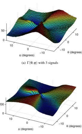
Fig. 3 presentsΓ(θ′_,ϕ′_)andH(θ′_,ϕ′_{)with 3 arriving}

signals of various parameters, to illustrate the continuity property of them. Fig. 3(a) presents the graph ofΓ(θ′_,ϕ′_),

whereas Fig. 3(b) presentH(θ′_,ϕ′_{). The result of 3 signals,}

whose direction and polarization parameter written in the form of(θ′,ϕ′,γ,η)are(−3,−4,12.5,30),(3,−3,45.5,50)

and(−3,4,70.5,70), is drawn in Fig. 3(a) and 3(b). It can be observed that in the two figures, theΓ(θ′,ϕ′)andH(θ′,ϕ′)

are continuous in most area, whereas the steep slopes occur near the directions of the impinging signals.

5.3 Precision and Resolution

Fig. 4, Fig. 5 and Fig. 6 provide stimulation results to compare the performances of the fast polarization MUSIC algorithm and other algorithms. The performance of the fast polarization MUSIC is compared with conventional MUSIC, and the rank reduction (RR) algorithm in [25, 26], which can be extended to arbitrary form of array as well. The performances of these algorithms are presented through Monte Carlo simulations.

−10 0

10

−10 0

10 0 50

θ (degrees)

φ (degrees)

(a) Γ(θ,ϕ)with 3 signals

−10 0

10

−10 0

10 0 200

θ (degrees)

φ (degrees)

(b)H(θ,ϕ)with 3 signals

Fig. 3.Polarization at all directions.

Fig. 4 draws snapshot numbers required to descry 2 close signals with various angle differences, calculated by (33) and (34). Their azimuth angles are 0◦, one signal’s elevation angle is set to 0◦, and the other is modified. The simulation is based on a UCA of 16 sensors, whose radius is 0.667 λ. The polarization parameters are(30,15)

and(50,100). In Fig. 4, the calculated results of the fast polarization MUSIC and conventional 2-D MUSIC are given according to the SNR. It can be seen that less snapshots are required to descry 2 close signals in the proposed algorithm, particularly with relatively low SNR.

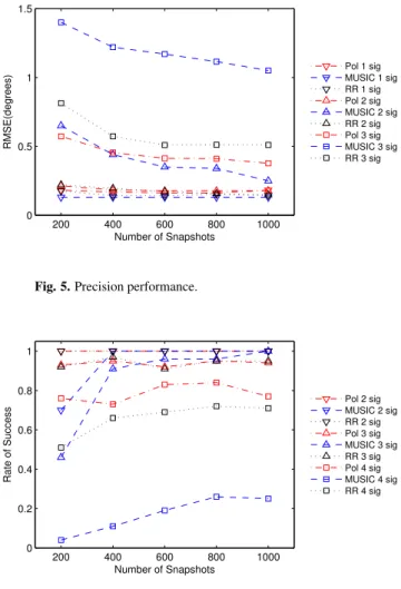
Fig. 5 compares different algorithms’ precision per-formance with various number of signals. RMSE stands for root mean square error. In Fig. 5, the estimation’s RMSE for the fast polarization MUSIC, conventional 2-D MUSIC and RR Algorithm are depicted. In 1-signal scenario, the signal’s parameters are (0.1,−3.1,12.5,30). In 2-signal scenario, the parameters are(0,−3.1,12.5,30)

and (0,3.2,60,60), whereas in the 3-signal scenario, they are (−3.1,−4.1,12.5,30), (3.3,−3.1,45.5,50) and

1 1.5 2 2.5 3 3.5 4 4.5 5 101

102 103 104

Difference in direction (degrees)

Threshold of snapshot number

Pol 15dB MUSIC 15dB Pol 20dB MUSIC 20dB Pol 25dB MUSIC 25dB

Fig. 4.Snapshot number required to resolve close signals.

200 400 600 800 1000

0 0.5 1 1.5

Number of Snapshots

RMSE(degrees)

Pol 1 sig MUSIC 1 sig RR 1 sig Pol 2 sig MUSIC 2 sig RR 2 sig Pol 3 sig MUSIC 3 sig RR 3 sig

Fig. 5.Precision performance.

200 400 600 800 1000

0 0.2 0.4 0.6 0.8 1

Number of Snapshots

Rate of Success

Pol 2 sig MUSIC 2 sig RR 2 sig Pol 3 sig MUSIC 3 sig RR 3 sig Pol 4 sig MUSIC 4 sig RR 4 sig

Fig. 6.Rate of success in resolution.

In Fig. 6, the success rates in multiple signals resolution are presented. The signals’ parameters are

(−6,−4.2,12.5,30), (3,−5.1,22.5,50), (−3,3.3,41,70)

and (6,6.2,62,90) in the 4-signal scenario. In other scenarios, they are the same as Fig. 5. Fig. 6 shows that the success rates of the fast polarization MUSIC are generally higher than that of conventional 2-D MUSIC and RR algorithm, particularly with small snapshot numbers.

Especially, the success rate of the proposed algorithm is approximately 80% in the 4-signal scenario, higher than that of RR algorithm and the conventional 2-D MUSIC.

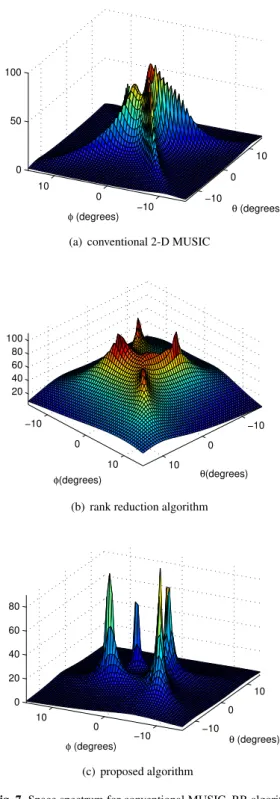
Figure 7 gives the space spectrum P(θ′,ϕ′) of the conventional 2-D MUSIC, the RR algorithm and the graph of PD(θ′,ϕ′)of the fast polarization MUSIC . The parameters

of the 4 incoming signals are the same as the 4-signal scenario in Fig. 6, with 500 snapshots. Fig. 7(a) shows that the peaks of the conventional 2-D MUSIC are eclipsed severely and cannot be distinguished. For the RR algorithm, the peaks in Fig. 7(b) can be located, although not very distinct. But in the space spectrum of the fast polarization MUSIC, all 4 peaks are quite clear.

5.4 Computation Complexity

In simulation results presented in this article, the ranges of azimuth and elevation are sampled with an interval of 0.5◦, and the ranges of azimuth and elevation angles are both limited from −15◦ to 15◦, i.e., θ′ _{∈[−15,15] and} ϕ′_{∈[−15,15]. Then the 2-D space spanned by azimuth and}

elevation will be sampled with 61×61=3721 samples, i.e., if the conventional MUSIC is adopted, 3721 points of the space spectrum are required to be calculated to estimate the arriving signals’ directions.

In the fast polarization MUSIC, suppose γ and η

are sampled with intervals of 3 degrees and 6 degrees, respectively. Based on the analysis in Subsection 4.3, the lower limit of sample number needed will be 5N1N2= 18605. When the worst case happens, the number becomes

(N3+N4)N1N2=338611, whereas the number of samples needed in the conventional 4-D polarization MUSIC is N1N2N3N4=6921060, approximately 20 times more than the worst case of the proposed algorithm.

Tab. 1 presents the average number of samples of space spectrum calculated in polarization MUSIC. The Monte Carlo experiments number is 100. The impinging signals’ parameters and the configuration of the array are the same as Fig. 5 and Fig. 6. The data in Tab. 1 shows that the average sample numbers is approximately 6N1N2, and is insensitive to the snapshot number and/or the signals’ number. So the calculation amount in the fast polarization MUSIC is as 6 times as that of conventional 2-D MUSIC needs. The fast polarization MUSIC has the same performance in precision and resolution as the original 4-D search polarization MUSIC, but the low computation complexity property makes it more attractive in practical application.

−10 0

10

−10 0

10 0 50 100

θ (degrees) φ (degrees)

(a) conventional 2-D MUSIC

−10

0

10 −10

0

10 20

40 60 80 100

θ(degrees) φ(degrees)

(b) rank reduction algorithm

−10 0

10

−10 0

10 0 20 40 60 80

θ (degrees) φ (degrees)

(c) proposed algorithm

Fig. 7.Space spectrum for conventional MUSIC, RR algorithm and the proposed algorithm.

Snapshots 200 400 600 800 1000 1 signal 23288 23432 23105 23203 23149 2 signals 22747 22843 22771 22866 22818 3 signals 22189 22236 22374 22241 22382 4 signals 21324 21302 21257 21149 21173

Tab. 1.Number of samples calculated in the proposed algo-rithm.

6. Conclusion

In this paper, a novel fast polarization MUSIC algorithm, which could reduce the considerable amount of computation, is proposed. Based on the fact that the difference of polarization between two close directions is minor or predictable, the daunting 4-D search is simplified by converting into two 2-D peak searches. The performance of fast polarization MUSIC is evaluated by theoretical analyses and simulations. It delivers improved precision and resolution with low computation complexity. The fact that this proposed algorithm is not confined to any specific pattern of polarization sensitive arrays expands its range of application.

Acknowledgements

The authors thank the support from National Natural Science Foundation of China (No. 61171180) for the research. We also gratefully acknowledge the assistance from Zhi-min Lin, Hong Hong, Zuo-liang Yin and Hui-jun Hou.

Appendix A: Proof of (32)

Define the noise space projection matrix as

PN=UNUHN. (46)

Using the expression given in [35], we have E_ˆ

PN−PN

=−

σ2

n

K tr(ΛSΓ

−2₎

PN+ (2M−2)

σ2

N

K USΛSΓ

−2_UH

S

(47)

whereKis the number of snapshots, ˆPNthe estimation ofPN

andσ2

N is the power of white noise. Elaborate (47) further,

we obtain: E_ˆ

PN−PN =−

σ2

N

K (ω1+ω2)PN

+(2M−2)σ

2

N

K ·(ω1u1u

H

1 +ω2u2uH2)

(48)

where ωi =λi/(λi−σ2N)2, i =1,2. According to the

definition of zero spectrumZ(θ,ϕ,γ,η), we have E_{Zˆ(θ,ϕ,γ,η)}=aHE_{PˆN}a

=

1−σ

2

N

K (ω1+ω2)

Z(θ,ϕ,γ,η) +e1+e2 (49)

wherea=a(θ,ϕ,γ,η), and

ei=ei(θ,ϕ,γ,η) =

(2M₋2)σ2

Nωi

K |a

H_u

i|2, i=1,2. (50)

The estimation of the zero spectrum of the first signal is E_{Zˆ(θ1,ϕ1,γ1,η1)}=e1(θ1,ϕ1,γ1,η1) +e2(θ1,ϕ1,γ1,η1)

where we use Z(θ1,ϕ1,γ1,η1) = 0. Similarly, the es-timation of the zero spectrum of the second one is E_{Zˆ(θ2,ϕ2,γ2,η2)}=e1(θ2,ϕ2,γ2,η2) +e2(θ2,ϕ2,γ2,η2).

At(θ0,ϕ0,γ0,η0), we have: E_{Zˆ(θ0,ϕ0,γ0,η0)}

=

1−σ

2

N

K (ω1+ω2)

Z(θ0,ϕ0,γ0,η0)

+e1(θ0,ϕ0,γ0,η0) +e2(θ0,ϕ0,γ0,η0).

(52)

Neglect the influence ofe1(θ,ϕ,γ,η), we get: Z(θ0,ϕ0,γ0,η0)>e2(θi,ϕi,γi,ηi)−e2(θ0,ϕ0,γ0,η0).

(53) The value of the zero spectrum at(θ0,ϕ0,γ0,η0)is:

Z(θ0,ϕ0,γ0,η0) =ka0k2− |aH0u1|2− |aH0u2|2 (54) whereai=a(θi,ϕi,γi,ηi), i=0,1,2.

Substitute (50) and (54) into (53), we have: ka0k2− |aH0u1|2− |aH0u2|2

>(2M−2)

K ·

λ2/σ2N

(λ2/σ2N−1)2

|aH_i u2|2− |aH0u2|2. (55)

Appendix B: Proof of (33) and (34)

λ2/σ2N

(λ2/σ2N−1)2

> 1

λ2/σ2N−1

≈ 1

ka0k2SNR1− |aH1a2|/(ka1k · kak)

(56)

where SNR is the signal-noise ratio of each signal. Substitute (56) into (32):

ka0k2− |aH0u1|2− |aH0u2|2

> 2(M−1)

|aH_ku2|2− |aH0u2|2

K_·SNR1− |aH₁a2|/(ka1k · ka2k) .

(57)

Then:

K> 2(M−1)

SNR ka0k2− |aH0u1|2− |aH0u2|2

· |a

H

ku2|2− |aH0u2|2 ka0k21− |aH₁a2|(ka1k · ka2k)

.

(58)

This is expression (33).

For the conventional MUSIC, the value of 1− |aH₁a2|/(ka1kka2k)is very close to zero, so the approxima-tion in (56) should be rewritten as:

λ2/σ2N

(λ2/σ2_N−1)2

≈ 1

SNR2ka0k41− |aH₁a2|/(ka1kka2k)2

.

(59)

The expression (57) becomes ka0k2− |aH0u1|2− |aH0u2|2

> (M−2)

|]aH_i u2|2− |aH0u2|2

K_·SNR2ka0k21− |aH1a2|/(kakka2k) 2.

(60)

Then in MUSIC, the required number of snapshots is:

K> (M−2)

|aH

i u2|2− |aH0u2|2 SNR2ka0k41− |aH₁a2|/(ka1kka2k)2

· 1

ka0k2− |aH0u1|2− |aH0u2|2

.

(61)

References

[1] BOHME, J. F. Estimation of source parameters by maximum likelihood and nonlinear regression. InAcoustics, Speech, and Signal Processing, IEEE International Conference on ICASSP’84. 1984, vol. 9, p. 271–274. DOI: 10.1109/ICASSP.1984.1172397

[2] BOHME, J. F. Estimation of spectral parameters of correlated signals in wavefields.Signal Processing, 1986, vol. 11, no. 4, p. 329–337. DOI: 10.1016/0165-1684(86)90075-7

[3] SCHMIDT, R. Multiple emitter location and signal parameter estimation.IEEE Transactions on Antennas and Propagation, 1986, vol. 34, no. 3, p. 278–280. DOI: 10.1109/TAP.1986.1143830

[4] ROY, R., PAULRAJ, A., KAILATH, T. ESPRIT-A subspace rotation approach to estimation of parameters of cisoids in noise. IEEE Transactions on Acoustics, Speech and Signal Processing, 1986, vol. 34, no. 5, p. 1340–1342. DOI: 10.1109/TASSP.1986.1164935

[5] OTTERSTEN, B., VIBERG, M., STOICA, P., NEHORAI, A.Exact and Large Sample ML Techniques for Parameter Estimation and Detection in Array Processing.New York: Springer-Verlag, 1993.

[6] RAO, B. D., HARI, K. V. S. Performance analysis of root-MUSIC.

IEEE Transactions on Acoustics, Speech and Signal Processing, 1989, vol. 37, no. 12, p. 1939–1949. DOI: 10.1109/29.45540

[7] ROY, R., KAILATH, T. ESPRIT-estimation of signal parameters via rotational invariance techniques.IEEE Transactions on Acoustics, Speech and Signal Processing, 1989, vol. 37, no. 7, p. 984–995. DOI: 10.1109/29.32276

[8] YARDIBI, T., LI, J., STOICA, P., CATTAFESTA III, L. N. Sparsity constrained deconvolution approaches for acoustic source mapping.

The Journal of the Acoustical Society of America, 2008, vol. 123, p. 2631. DOI: 10.1121/1.2896754

[9] YARDIBI, T., LI, J., STOICA, P., XUE, M., BAGGEROER, A. B. Source localization and sensing: A nonparametric iterative adaptive approach based on weighted least squares.IEEE Transactions on Aerospace and Electronic Systems, 2010, vol. 46, no. 1, p. 425–443. DOI: 10.1109/TAES.2010.5417172

[10] MISHALI, M., ELDAR, Y.C., ELRON, A. J. Xampling: Signal acquisition and processing in union of subspaces.IEEE Transactions on Signal Processing, 2011, vol. 59, no. 10, p. 4719–4734. DOI: 10.1109/TSP.2011.2161472

[12] ELKADER, S. A., GERSHMAN, A. B., WONG, K. M. Rank reduction direction-of-arrival estimators with an improved robust-ness against subarray orientation errors. IEEE Transactions on Signal Processing, 2006, vol. 54, no. 5, p. 1951–1955. DOI: 10.1109/TSP.2006.872321

[13] RUBSAMEN, M., GERSHMAN, A. B. Direction-of-arrival es-timation for nonuniform sensor arrays: from manifold sepa-ration to Fourier domain MUSIC methods. IEEE Transactions on Signal Processing, 2009, vol. 57, no. 2, p. 588–599. 10.1109/TSP.2008.2008560

[14] KAVEH, M., BARABELL, A. The statistical performance of the MUSIC and the minimum-norm algorithms in resolving plane waves in noise. IEEE Transactions on Acoustics, Speech and Signal Processing, 1986, vol. 34, no. 2, p. 331–341. DOI: 10.1109/TASSP.1986.1164815

[15] STOICA, P., ARYE, N. MUSIC, maximum likelihood, and Cramer-Rao bound.IEEE Transactions on Acoustics, Speech and Signal Processing, 1989, vol. 37, no. 5, p. 720–741. DOI: 10.1109/29.17564 [16] NEHORAI, A., PALDI, E. Vector-sensor array processing for elec-tromagnetic source localization.IEEE Transactions on Signal Pro-cessing, 1994, vol. 42, no. 2, p. 376–398. DOI: 10.1109/78.275610 [17] LI, J., COMPTON, J. Angle and polarization estimation using

ESPRIT with a polarization sensitive array.IEEE Transactions on Antennas and Propagation, 1991, vol. 39, no. 9, p. 1376–1383. DOI: 10.1109/8.99047

[18] LI, J., COMPTON, J. Two-dimensional angle and polarization estimation using the ESPRIT algorithm. IEEE Transactions on Antennas and Propagation, 1992, vol. 40, no. 5, p. 550–555. DOI: 10.1109/8.142630

[19] HUA, Y. A pencil-MUSIC algorithm for finding two-dimensional angles and polarizations using crossed dipoles.IEEE Transactions on Antennas and Propagation, 1993, vol. 41, no. 3, p. 370–376. DOI: 10.1109/8.233122

[20] HO, K.-C, TAN, K.-C., TAN, B. T. G. Efficient method for estimating directions-of-arrival of partially polarized signals with electromag-netic vector sensors.IEEE Transactions on Signal Processing, 1997, vol. 45, no. 10, p. 2485–2498. DOI: 10.1109/78.640714

[21] HO, K.-C., TAN, K.-C., NEHORAI, A. Estimating directions of arrival of completely and incompletely polarized signals with elec-tromagnetic vector sensors.IEEE Transactions on Signal Processing, 1999, vol. 47, no. 10, p. 2845–2852. DOI: 10.1109/78.790664

[22] ZOLTOWSKI, M., WONG, K. ESPRIT-based 2-D direction finding with a sparse uniform array of electromagnetic vector sensors.IEEE Transactions on Signal Processing, 2000, vol. 48, no. 8, p. 2195– 2204. DOI: 10.1109/78.852000

[23] HE, J., LIU, Z. Computationally efficient 2D direction finding and polarization estimation with arbitrarily spaced electromagnetic vector sensors at unknown locations using the propagator method.

Digital Signal Processing, 2009, vol. 19, no. 3, p. 491–503. DOI: 10.1016/j.dsp.2008.01.002

[24] RAHAMIM, D., TABRIKIAN, J., SHAVIT, R. Source localization using vector sensor array in a multipath environment. IEEE Transactions on Signal Processing, 2004, vol. 52, no. 11, p. 3096– 3103. DOI: 10.1109/TSP.2004.836456

[25] WEISS, A. J., FRIEDLANDER, B. Direction finding for diversely polarized signals using polynomial rooting.IEEE Transactions on Signal Processing, 1993, vol. 41, no. 5, p. 1893–1905. DOI: 10.1109/78.215307

[26] WONG, K., LI, L., ZOLTOWSKI, M. D. Root-MUSIC-based direction-finding and polarization estimation using diversely po-larized possibly collocated antennas.IEEE Antennas and Wireless Propagation Letters, 2004, vol. 3, no. 1, p. 129–132. DOI: 10.1109/LAWP.2004.831083

[27] MIRON, S., GUO, X., BRIE, D. DOA estimation for polarized sources on a vector-sensor array by PARAFAC decomposition of the fourth-order covariance tensor. InProceedings of the EUSIPCO. 2008, p. 25–29.

[28] GONG, X., LIU, Z., XU, Y., ISHTIAQ, A. Direction-of-arrival estimation via twofold mode-projection. Signal Processing, 2009, vol. 89, no. 5, p. 831–842. DOI: 10.1016/j.sigpro.2008.10.034

[29] YUAN, Q., CHEN, Q., SAWAYA, K. MUSIC based DOA finding and polarization estimation using USV with polarization sensitive array antenna. In IEEE Radio and Wireless Symposium. 2006, p. 339–342. DOI: 10.1109/RWS.2006.1615164

[30] LIU, S., JIN, M., QIAO, X. Joint polarization-DOA estimation using circle array. InIET International Radar Conference. 2009, p. 1–5. [31] COSTA, M., KOIVUNEN, V., RICHTER, A. Azimuth, elevation,

and polarization estimation for arbitrary polarimetric array configu-rations. InStatistical Signal Processing.Cardiff (UK), 2009, p. 261– 264. DOI: 10.1109/SSP.2009.5278590

[32] COSTA, M., RICHTER, A., KOIVUNEN, V. DoA and polarization estimation for arbitrary array configurations. IEEE Transactions on Signal Processing, 2012, vol. 60, no. 5, p. 2330–2343. DOI: 10.1109/TSP.2012.2187519

[33] YANG, P., YANG, F., NIE, Z., ZHOU, H., LI, B., TANG, X. Fast 2-d DOA and polarization estimation using arbitrary conformal antenna array. Progress In Electromagnetics Research C, 2012, vol. 25, p. 119–132. DOI: 10.2528/PIERC11070706

[34] GUO, R., MAO, X., LI, S., LIN, Z. Fast four-dimensional joint spectral estimation with array composed of diversely polarized elements. InIEEE Radar Conference (RADAR).2012 , p. 919–923. DOI: 10.1109/RADAR.2012.6212268

[35] FRIEDLANDER, B., WEISS, A. J. The resolution threshold of a direction-finding algorithm for diversely polarized arrays.IEEE Transactions on Signal Processing, 1994, vol. 42, no. 7, p. 1719– 1727. DOI: 10.1109/78.298279

[36] ZHOU, C., HABLER, F., JAGGARD, D. L. A resolution measure for the MUSIC algorithm and its application to plane wave arrivals contaminated by coherent interference.IEEE Transactions on Signal Processing, 1991, vol. 39, no. 2, p. 454–463. DOI: 10.1109/78.80829 [37] STOICA, P., NEHORAI, A. MUSIC, maximum likelihood, and Cramer-Rao bound: further results and comparisons. IEEE Transactions on Acoustics, Speech and Signal Processing, 1990, vol. 38, no. 12, p. 2140–2150. DOI: 10.1109/29.61541

[38] HUDSON, J. E.Adaptive Array Principles.Peter Peregrinus Press, 1981.

About the Authors . . .

Ran GUOwas born in Dalian, Liaoning Province, China. He received his M.Sc. from HIT (Harbin Institute of Tech-nology) in 2009. His research interests include array signal processing, polarization sensitive array and super-resolution DOA estimation. Email: guoran1112@gmail.com.