Parameterization and uncertainty in coupled ecohydrological models

(1)

HESSD

6, 4155–4207, 2009

Coupled ecohydrological

models

S. Arnold et al.

Title Page

Abstract Introduction

Conclusions References

Tables Figures

◭ ◮

Back Close

Full Screen / Esc

Printer-friendly Version

Interactive Discussion Hydrol. Earth Syst. Sci. Discuss., 6, 4155–4207, 2009

www.hydrol-earth-syst-sci-discuss.net/6/4155/2009/ © Author(s) 2009. This work is distributed under the Creative Commons Attribution 3.0 License.

Hydrology and Earth System Sciences Discussions

Papers published inHydrology and Earth System Sciences Discussionsare under open-access review for the journalHydrology and Earth System Sciences

Parameterization and uncertainty

in coupled ecohydrological models

S. Arnold1, S. Attinger1,3, K. Frank2, and A. Hildebrandt1 1

Department Computational Hydrosystems, UFZ – Helmholtz Centre for Environmental Research, Leipzig, Germany

2

Department of Ecological Modelling, UFZ – Helmholtz Centre for Environmental Research, Leipzig, Germany

3

Friedrich-Schiller-University of Jena, Institute of Geosciences, Jena, Germany

Received: 22 May 2009 – Accepted: 31 May 2009 – Published: 9 June 2009

Correspondence to: S. Arnold (sven.arnold@ufz.de)

Published by Copernicus Publications on behalf of the European Geosciences Union.

(2)

HESSD

6, 4155–4207, 2009

models

S. Arnold et al.

Title Page

Tables Figures

◭ ◮

Back Close

Full Screen / Esc

Interactive Discussion

Abstract

In this paper we develop and apply a conceptual ecohydrological model to investigate the effects of model structure and parameter uncertainty on the prediction of vegetation structure and hydrological dynamics. The model is applied for a typical water limited riparian ecosystem along an ephemeral river: the middle section of the Kuiseb River

5

in Namibia. We modelled this system by coupling an ecological model with a con-ceptual hydrological model. The hydrological model is storage based with stochastical forcing from the flood. The ecosystem is modelled with a population model, and repre-sents three dominating riparian plant populations. In appreciation of uncertainty about population dynamics, we applied three model versions with increasing complexity.

Pop-10

ulation parameters were found by Latin Hypercube sampling of the parameter space and with the constraint that three species should coexist as observed. Two of the three models were able to reproduce the observed coexistence. However, both models relied on different coexistence mechanisms, and reacted differently to change of long term memory in the flood forcing. The coexistence requirement strongly constrained the

15

parameter space for both successful models. Only very few parameter sets (0.5% of 150 000 samples) allowed for coexistence in a representative number of repeated sim-ulations (at least 10 out of 100) and the success of the coexistence mechanism was controlled by the combination of population parameters. The average values of hydro-logic variables like transpiration and depth to ground water were similar for both

mod-20

els, suggesting that they were mainly controlled by the applied hydrological model. The fluctuations of depth to groundwater and transpiration, however, differed significantly, suggesting that they were controlled by the applied ecological model and coexistence mechanisms. Our study emphasizes that uncertainty about ecosystem structure and intra-specific interactions influence the prediction of the hydrosystem.

25

(3)

HESSD

6, 4155–4207, 2009

models

S. Arnold et al.

Title Page

Tables Figures

◭ ◮

Back Close

Full Screen / Esc

Interactive Discussion

1 Introduction

In semiarid environments water is not only a scarce resource, water availability also varies greatly in timing and magnitude. Both natural ecosystems and people have to adapt to these conditions, and often they share the same water source. Thus, wa-ter management of the wawa-ter source might influence natural ecosystems, but also

in-5

versely, the management of vegetation might affect the water fluxes. In order to un-derstand, what implications human development in semiarid regions has, models are required that help investigating the effect of management actions. Such models need appropriate description of both ecological and hydrological processes.

A great deal of work in ecohydrology has already been dedicated to

understand-10

ing mechanisms, by which a variation in water availability influences vegetation pat-terns. Much of this work is based on considering single plant species, and compar-ing expected water stress-levels in different environments. Therefore, these models cannot consider inter-specific competition or coexistence. However, research deal-ing with biodiversity and species-co-existence suggests that particularly fluctuations of

15

environmental signals might favour co-existence (D’Odorico et al., 2008). Hence cer-tain levels of variance of water availability could also be a driver for maincer-taining multi-species plant communities. Moreover, diverse ecosystems are thought to be more re-silient to disturbance and should thus react differently to extreme conditions than single species ecosystems. Hence coexistence mechanisms might be important ecosystem

20

processes shaping plant-water interactions in water limited environments, which moti-vates the need for multispecies ecohydrological models. Such a model is developed and applied in this paper.

Ecological modelling has different approaches to describe multi-species plant com-munities. One way is spatially explicit individual-based modelling (DeAngelis and

25

Gross, 1992; Grimm and Railsback, 2005), representing a bottom-up approach. Here, plant communities are described as systems of interacting plant individuals responding to their environment. This approach is particularly powerful when specific systems are

(4)

HESSD

6, 4155–4207, 2009

models

S. Arnold et al.

Title Page

Tables Figures

◭ ◮

Back Close

Full Screen / Esc

Interactive Discussion to be analysed. The respective models, however, are often complex that makes

param-eterization a challenge (lots of parameters) and hampers generalization (adjustment to a specific case vs. principle understanding, transferability). To gain principle under-standing of the interplay between water resources and vegetation and the response of environmental variability along ephemeral rivers is central for the present study.

There-5

fore, we follow a top-down approach, i.e. we use a multi-species population dynamical model (Kot, 2001) to describe the plant community in an aggregated way but explic-itly consider the species’ competition for water. The population dynamical parameters summarize all relevant effects caused at the individual scale (Moorcroft, 2003; Frank and Wissel, 2002; Fahse et al., 1998; Heinz et al., 2005; Ovaskainen and Hanski,

10

2002, 2004). Most ecohydrological models work at the population scale (Rodriguez-Iturbe et al., 2001; Porporato et al., 2001; Camporeale and Ridolfi, 2006; Ridolfi et al., 2000). Direct parameterization of population models is sometimes impossible as this requires long-term observation of species abundance, which is not always available.

Generally, both population and hydrological models can be developed with varying

15

levels of complexity. In order to keep a coupled model manageable, the level of model complexity needs to be appropriate regarding the desired predicted variable but also regarding the available data. And there has to be a strategy how the model should be parameterized.

In this study, we address this parameterization problem by using pattern-oriented

20

modelling, in that we adjust species parameters such that the resulting model repro-duces the observed coexistence. Models have been parameterized based on infor-mation of presence or absence of plant species before. When the existence criterion will be extended to several species it is called coexistence, and also observed coexis-tence has been used to evaluate (at least qualitatively) the validity of ecohydrological

25

models (Laio et al., 2001; Rodriguez-Iturbe et al., 1999). In doing so, researchers put their models to a strict test, since modelling coexistence is comparatively difficult (Arora and Boer, 2006; Clark et al., 2007). It is required, that mechanisms supporting coexis-tence are related through precise order of parameter combinations. A given model only

(5)

HESSD

6, 4155–4207, 2009

models

S. Arnold et al.

Title Page

Tables Figures

◭ ◮

Back Close

Full Screen / Esc

Interactive Discussion allows for coexistence, if its parameters meet certain conditions. A number of

mech-anisms can be invoked fostering coexistence in models, such as ecological niches (in time and space) and tradeoffs (Chesson, 2000; Clark et al., 2007). Ecological theory also indicates that the variability of an environmental signal, such as resources or dis-turbance regimes, influences biodiversity. According to the Intermediate Disdis-turbance

5

Hypothesis (Connell, 1978; Huston, 1979), moderate levels of environmental fluctua-tions can enhance both biodiversity and resilience (D’Odorico et al., 2008). So far, such studies have dealt with uncorrelated, random environmental signals. However, many hydrologic time series are characterized by auto-correlated and longterm-memory pro-cesses (Montanari et al., 1997; Hurst, 1951), particularly in arid environments. This

10

directly leads to the question of the role of this autocorrelation, that is the duration of a disturbance event (water stress, disruptive flood), for the functioning of the ecohy-drological system. Moreover, studies usually consider only one consequence of an environmental signal. However, the same signal, for example rain, may interact with the system in multiple ways. A strong rain event might recharge the water storage for

15

plants, but at the same time, the storm might destroy part of the vegetation. Thus the event acts on both, mortality and growth, but possibly not in the same fashion. Such combined effects are not fully understood so far. In this work we wish to investigate both of these issues, based on the example of an ephemeral river in Namibia. This allows for testing the adequateness of the Intermediate Disturbance Hypothesis in the

20

context of ecohydrological systems along ephemeral rivers.

The middle section of the ephemeral Kuiseb River in Namibia is a representative example of an environmental system with ecohydrological feedbacks and need for management. Previous studies indicate that the development of riparian vegetation depends on the subsurface water storage (alluvial aquifer) which is recharged by

inter-25

mittent floods. At the same time, strong floods lead to uprooting of riparian vegetation and increased mortality. There is no rainfall in this part of the river, the floods originate in the upper reach, and depend both on the rainfall regime and small scale farm dams. In this study, we aim to build a model that allows understanding, how the flood regime

(6)

HESSD

6, 4155–4207, 2009

models

S. Arnold et al.

Title Page

Tables Figures

◭ ◮

Back Close

Full Screen / Esc

Interactive Discussion interacts with the riparian ecosystem and the resulting transpiration loss and aquifer

storage. Little data is available regarding the ecosystem. We therefore rely on concep-tual models both for ecosystem and aquifer. In order to address structural uncertainty, we select three models, with increasing degree of complexity of the ecological model. We attempt to parameterize these models based on the scarce available information,

5

namely the fact that three species coexist and some knowledge about their maximum transpiration rates and rooting behaviour. Our investigation shows that different coexis-tence supporting mechanisms can be invoked, depending on the assumed conceptual model. While the mean hydrologic variables (groundwater level and transpiration) were similar in all models, their variability depended both on the model structure and the

10

parameters sets. This points at the difficulty to parameterize an ecohydrological model in real world applications. However, our model gives clear indications, what measure-ments are most effective for improving the necessary process understanding.

2 Methods and materials

2.1 Study site

15

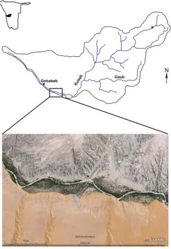
The study site covers an area of approximately 18 km2 and is located in the Kuiseb catchment (∼15 500 km2, Jacobson et al., 1995) in Namibia (Fig. 1). The Kuiseb River arises from the Khomas Hochland (∼2000 m in elevation) and runs westward through the escarpment into the Atlantic Ocean. The rainy season is during the southern hemi-sphere summer between January and April (Henschel et al., 2005). Most of the rain

20

falls in the upper reach of the catchment (Khomas Hochland). This study is concerned with the arid middle reach of the Kuiseb River, where rain is exceptional, and water arrives mainly during the floods in the ephemeral river channel. Near this channel, riparian vegetation has established. Although the channel does not contain water for most of the year, it supplies a shallow aquifer with water during times of flood and thus

25

creates a living environment for riparian vegetation. The flood is influenced by

(7)

HESSD

6, 4155–4207, 2009

models

S. Arnold et al.

Title Page

Tables Figures

◭ ◮

Back Close

Full Screen / Esc

Interactive Discussion stream farm damns and the ground water table is influenced both by plants and human

consumption.

2.1.1 Ecosystem

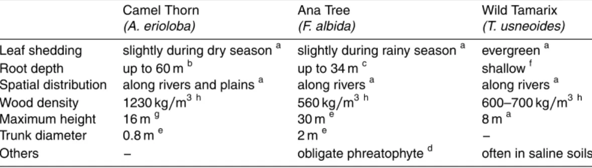
Vegetation around the river channel consists to 80% of only three coexisting species: Camel Thorn (Acacia erioloba), Ana Tree (Faidherbia albida) and Wild Tamarix

5

(Tamarix usneoides) (Theron et al., 1980). All of them depend on the infiltration of flood water, with slight differences in strategies. Schachtschneider and February (2007) in-vestigated the water use strategies of all three species by using isotope methods. They found that both Camel Thorn and Ana Tree use a mixture of ground- and soil water, and Wild Tamarix uses water from the unsaturated zone, originating from flood and

10

also fog water. The known differences between the three species are in their phenol-ogy (time of leaf shedding), maximum transpiration and growth rates (see Table 1). Besides supplying vegetation with water, floods in the river channel have also a de-structive component. Small trees are usually washed out by strong floods. The latter makes slow growing trees vulnerable for large floods for longer time.

15

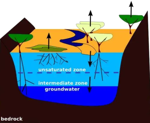
2.1.2 Hydrosystem

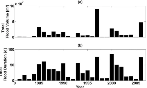
The study site is located in a hyperarid area with mean annual rainfall less than 20 mm and mean potential evaporation of 1700 to 2500 mm (Botes et al., 2003). The shallow alluvial aquifer consists of sand and is embedded into impermeable granite (Dahan et al., 2008) (Fig. 2). Its thickness and width vary along the river. The alluvial aquifer is

20

recharged by temporary floods that are caused by rainfall in the upper Kuiseb catch-ment (Khomas Hochland). Volume and duration of the resulting floods vary strongly (Fig. 3). Larger floods burst over the limits of channel bed, leading to inundation of the river banks. At the same time, about 90% of the floods run dry within the Kuiseb middle section under study here. This shows the comparatively large role of

infiltra-25

tion. The dynamics of flood water infiltration were investigated by Dahan et al. (2008).

(8)

HESSD

6, 4155–4207, 2009

models

S. Arnold et al.

Title Page

Tables Figures

◭ ◮

Back Close

Full Screen / Esc

Interactive Discussion Their studies show that, during a flood, the water content of the unsaturated layer only

increases up to the twofold value of the field capacity and that the infiltration fluxes are very similar although each flood is characterized by different flow conditions. Further, above a certain flood stage threshold, it is the flow duration and not the flood height that controls the recharge amounts.

5

2.2 Hydrological model

We modelled the hydrological processes along an ephemeral river with shallow aquifer. Figure 2 gives a sketch of the hydrological unit modelled. We modelled a representative river-valley segment of 60 km length and a constant width of 300 m. Hence we consid-ered total fluxes over the entire surface area of the segment, which isAseg=18 km

2 .

10

The water balance for this segment is written as Eq. (1)

∆W S(t)= ∆(S)_unsat(t)+ ∆SGW(t), (1) where∆W S(t) is the sum of change in unsaturated (∆Sunsat(t)) and ground water stor-age (∆SGW(t)). The storage in the unsaturated and ground water layer was calculated as

15

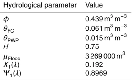
Sunsat(t)=Aseg·zunsat(t)·θ(t) for the unsaturated storage, (2a) SGW(t)=Aseg·hGW(t)·φ for the ground water storage, (2b) whereθ(t) is the water content (m3/m3) of the unsaturated zone, which ranges be-tween 0 and porosityφ(Table 2) and hGW(t) is the ground water level. The depth to ground waterzunsat(t) is

20

zunsat(t)=hWS−hGW(t), (3)

wherehWS=15 m is the total depth of the alluvium. In our simulations we fixed the initial value of ground water depth tozunsat(t=1)=5 m.

(9)

HESSD

6, 4155–4207, 2009

models

S. Arnold et al.

Title Page

Tables Figures

◭ ◮

Back Close

Full Screen / Esc

Interactive Discussion The change in unsaturated storage was calculated as

∆Sunsat(t)=I(t)−GW R(t)−Tunsat(t), (4) withI(t) denoting the infiltration,GW R(t) the ground water recharge, andTunsat(t) the transpiration from the unsaturated storage. The infiltration to unsaturated soil is based on the results of Dahan et al. (2008) who concluded that infiltration fluxes are limited

5

by a flux-regulating mechanism at the top of the unsaturated zone, independent of the flood height. They suggest a time constant infiltration rate ofQ_I(t)=2400 m3/d ha. Therefore, the infiltration depends only on flood durationD(t) (Eq. 20) and the specific infiltration fluxQI(t):

I(t)=D(t)·Q_I(t). (5)

10

Flood durations is calculated as a function of flood volume in Eq. (20) (see Sect. 2.3). The ground water recharge depends on the water contentθ(t) of the unsaturated layer:

GW R(t)=Sunsat(t)−SFC(t) forφ≥θ(t)≥θFC(t), (6a)

GW R(t)=0 forθ(t)≤θFC(t). (6b)

whereSFC(t) is the water volume in the unsaturated zone corresponding to the water

15

content at field capacity (θFC(t)=0.061). The transpiration is composed of transpiration from unsaturated layer and ground water. The transpiration from the unsaturated layer is the sum of the transpiration from individual speciesTunsat,i(t):

Tunsat,i(t)=max

"

(Sunsat(t)−SPWP(t)), 3 X

i=1

Tunsat,i(t)

#

. (7a)

For plants where the roots reach the groundwater, transpiration originates from both

20

the unsaturated and the saturated zone. The unsaturated part is calculated as

Tunsat,i(t)=

Vunsat,i(t)

VWS,i(t)

TWS,i(t), (7b)

(10)

HESSD

6, 4155–4207, 2009

models

S. Arnold et al.

Title Page

Tables Figures

◭ ◮

Back Close

Full Screen / Esc

Interactive Discussion whereSPWP(t) is the water volume in the unsaturated zone corresponding to the water

content at permanent wilting point (θPWP(t)=0.015),TWS,i(t) the transpirational demand

for each species Eq. (10),Vunsat,i(t) the water volume in the unsaturated storage and

VWS,i(t) is the total water volume (unsaturated and ground water) that can be reached

by plant roots of speciesi:

5

VWS,i(t)=Vunsat,i(t)+VGW,i(t), (8)

whereVGW,i(t) is the ground water volume available by plant roots. The water in the

unsaturated storage available for transpiration of speciesi depends on its rooting depth zr,i(t):

Vunsat,i(t)=zr,i(t)·θ(t)·Aseg if zr,i ≤zunsat(t), (9a)

10

Vunsat,i(t)=zunsat(t)·θ(t)·Aseg if zr,i > zunsat(t), (9b) The transpirational demand for each species (TWS,i(t)) is a linear function of the green

biomassGi(t) (see Sect. 2.4) with an upper boundary given by the potential

evapotran-spiration (PET):

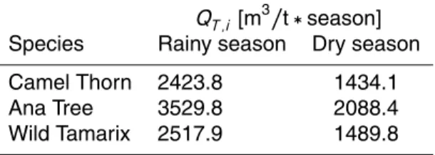
TWS,i(t)=max PET, QT,i(t)·Gi(t)

. (10)

15

The PET was estimated using the Penman-Monteith Equation for both the flooding and the dry season. The transpiration per green biomassQT,i(t) of each species is derived

from measurements of Bate and Walker (1991) and is summarized in Table 3. The change in ground water was calculated as

∆SGW(t)=GW R(t)+QGW(t)−TGW(t), (11)

20

whereQGW(t) is the ground water flow andTGW(t) the transpiration of all species from ground water Eq. (14). The ground water flow is

QGW(t)=QIn+QL−QOut(t)−QV, (12)

(11)

HESSD

6, 4155–4207, 2009

models

S. Arnold et al.

Title Page

Tables Figures

◭ ◮

Back Close

Full Screen / Esc

Interactive Discussion whereQIn is the ground water inflow from upstream,QOut(t) the ground water outflow

downstream,QLthe lateral ground water inflow, and QVthe vertical ground water out-flow to the bedrock. QIn,QLand QV are assumed to be constant over time (Table 7). QOut(t) was calculated by Darcy’s Law, as:

QOut(t)=kf ·∆h(t)·AGW (13)

5

with k_f denoting the hydraulic permeability of the ground water layer, ∆h(t) the hy-draulic gradient between the inlet and outlet of the modelled aquifer segment, andA_GW the cross-sectional area of the ground water layer. The transpiration of all species from ground water is the sum of individual species transpirationsTGW,i(t):

TGW(t)=max "

(SGW(t)−SPWP(t)) 3 X

i=1

TGW,i(t)

#

, (14a)

10

TGW,i(t)=

VGW,i(t)

VWS,i(t)

TWS,i(t), (14b)

whereVGW,i(t) is the ground water that can be reached by plant roots of speciesi.

In the water balance described above, we neglected two processes: precipitation and evaporation. The first is very low at the study site (23.8 mm/year at Gobabeb Research Centre; Schulze, 1969). The second is only active during flooding, which

15

is only a few days per year. The effective depth of direct evaporation from bare soils was assumed to be 1.5 m and can be considered as non active soil layer above the alluvium.

2.3 The stochastic flood generator

The flood volumeVFlood(t) was generated by a fractional autoregressive moving

aver-20

age (FARIMA(p, d , q), p, q∈N) model with symmetric α-stable (SαS, α∈(1,2)) inno-vations (Kokoszka and Taqqu, 1995; Stoev and Taqqu, 2004). The FARIMA(p, d , q) model generates time series with both short- and long-term dependence structures

(12)

HESSD

6, 4155–4207, 2009

models

S. Arnold et al.

Title Page

Tables Figures

◭ ◮

Back Close

Full Screen / Esc

Interactive Discussion that are present in many hydrologic processes (Montanari et al., 1997; Hurst, 1951).

We used the algorithm presented in (Stoev and Taqqu, 2004) to generate time series with given short- and long-term memory. The short term dependence structure is de-termined by the real polynomialsX_pand Ψq of degreep and q. The autoregressive

part of FARIMA is represented by the coefficients ofXp, 5

Xp(λ)=1−χ1λ−χ2λ2−...−χpλp, (15)

whereX1(λ) =1−0.192λandλis a random number drawn from a normal distribution with mean 0 and standard deviation 1. The moving average part is represented by the coefficients ofΨq:

Ψq(λ)=1−ψ1λ−ψ2λ2−...−ψpλp, (16) 10

withΨ1(λ)=1−0.8969λ. The long term behaviour is governed bydthat is an arbitrary fractional real number:

0< d <1−1/α, and 1< α <2. (17)

The relationship betweend and the Hurst-ExponentH is as follows:

H =d+1/α . (18)

15

The value of H varies between 0 and 1, an H of 0.5 means absence of long term memory or white noise. Values lower than 0.5 correspond to negative dependence; however, these are rarely encountered in the analysis of hydrologic data (Montanari et al., 1997). Typical values of H range between 0.7 and 0.8 (Hurst, 1951). Hence, for our study, we assumedH to be 0.75 (withα=1.99 andd=0.25), andp=q=1. The time

20

series were generated with FARIMA(p=1, d=0.25, q=1) and adjusted to the observed mean annual flood volumeµFlood=3 269 000m

3

, and thus yielding

VFlood(t)=e(FARIMA(1,0.25,1)+log(µFlood)). (19)

(13)

HESSD

6, 4155–4207, 2009

models

S. Arnold et al.

Title Page

Tables Figures

◭ ◮

Back Close

Full Screen / Esc

Interactive Discussion Flood duration was found to be related to flood volume. Therefore we performed a

lin-ear regression between the measured flood duration and the corresponding logarithmic flood volumes from 1981 to 2006. The derived best fit (r2=0.9) was given by

D(t)=elog

V_Flood(t)−10.58

1.64 , (20)

and used in the following to calculate the flood duration.

5

2.4 Ecological model

The ecological model aims to describe the dynamics of the plant community consisting of the three tree species of interest in the river-basin of the Kuiseb in relation to the availability of water as jointly utilized resource. Each tree species is characterized by its biomass in the river-valley segment. In order to address important processes

10

of the plant community dynamics and their response to the hydrological system in an adequate way, biomass of a species is differentiated into green (G) and reserve biomass (R) similarly as (Muller et al., 2007), who termedRafter (Noy-Meir, 1982). The green biomass describes all the parts of a plant, which perform photosynthesis, while the reserve biomass covers all parts of the plant that are not photosynthetically active,

15

like woody parts and roots. The dynamic ofGis driven by seasonality (phenology) and short-term water stress. The process of photosynthesis performed byG depends on the availability of water (transpiration, see Sect. 2.2) and results in the production of organic carbon, which maintains both green and reserve biomass. The dynamic ofR occurs on a longer timescale and reflects the long-term history of the ecohydrological

20

system.

The model is applied at a seasonal time scale, thus dividing the year in two halves: the season when floods occur (southern hemisphere summer) and the dry season. During the seasons, when the plants are photosynthetically active, the green biomass G_i is modelled as

25

Gi(t)=(1−εi(t))·Gi(t−1)+wG,i(t)·Ri(t−1), (21)

(14)

HESSD

6, 4155–4207, 2009

models

S. Arnold et al.

Title Page

Tables Figures

◭ ◮

Back Close

Full Screen / Esc

Interactive Discussion whereG_i(t) and G_i(t−1) are the green biomass in this and the previous time step of

speciesi, with units of t/ha,Ri(t−1) is the reserve biomass in the previous time step,

w_G,i(t) is the conversion rate from reserve into green biomass Eq. (24), and ε_i(t) is the unitless water stress function Eq. (25), ranging from 0 for no water stress to 1 for complete water stress. The latter two terms,wG,i(t) andεi(t), are functions of the 5

available amount of water (Eqs. 24 and 25). The first term of Eq. (21), (1−ε_i(t))·G_i(t−1), denotes the leaf shed due to water stress, while the second part, w_G,i(t) ·R_i(t−1), denotes the growing of leaves from the existing reserve biomass.

Depending on the complexity of the model, we either assume no phenological dif-ferences between the species (model A), or we include the known differences in

phe-10

nology. In the first case, Eq. (21) applies to all species at all times. In the latter case, some species are dormant during a particular season (model B and C). Green biomass during the dormant season was calculated as:

G_i(t)=(1−l s_i)·(1−ε_i(t))·G_i(t−1), (22) wherel s_i is the unitless leaf shedding factor and ranges from 0 to 1 of speciesi.l s_i=0

15

corresponds to no leaf shedding at all, and 1 to complete leaf shed. Usually, leaf shed is not complete, sol si takes a value between 0 and 1.

The formation of reserve biomass takes place at the end of each seasont:

R_i(t)=fr_i(t)·

1−m_R,i ·(1−ε_i(t))

·R_i(t−1)+w_R,i·G_i(t) (23) wherefr_i(t) is the unitless flood resistance of speciesi and ranges from 0 to 1 (Eq. 26),

20

see below). It denotes the vulnerability of a given species to being uprooted and washed away by a flood of given magnitude.fri(t)=0 corresponds to complete removal

of reserve biomass by the flood. In the dry season, fr_i(t) is set to 1. The parame-term_R,i denotes the mortality of the reserve biomass, andw_R,i the rate of conversion from green into reserve biomass. Both are constant over time and unitless. The first

25

part of Eq. (23), [1−m_R,i(1−ε_i(t))]·R_i(t−1), denotes the amount of reserve biomass remaining after mortality and response to water stress. Note that the total mortality in-creases whenεi(t)>0. The second part,wR,i·Gi(t), corresponds to growth of reserve

(15)

HESSD

6, 4155–4207, 2009

models

S. Arnold et al.

Title Page

Tables Figures

◭ ◮

Back Close

Full Screen / Esc

Interactive Discussion biomass, based on the photosynthesis performed by the green biomassG_i(t). In our

simulations we fixed the initial values of green and reserve biomass toGi(t=1)=0 t/ha

andR_i(t=1)=0.1 t/ha.

In our model, favourable periods of growth in the green biomass G can markedly increase the reserve biomassR, whereas unfavourable periods reduce G fast, butR

5

only slowly. In his paper about the multispecies competition in variable environments, Chesson (1994) called this the storage effect, which “is a metaphor for the potential for periods of strong positive growth that cannot be cancelled by negative growth at other times”. The storage effect is enhanced by the parameterw_R,i (Eq. 23).

The three parameters conversion ratew_G,i(t), water stressε_i(t), and flood resistance

10

fr_i(t) are characteristics of the tree species that are dynamically linked to the hydrosys-tem. The conversion rate from reserve to green biomass,w_G,i(t),is described by a sig-moid function that depends on the water volume in the alluvium that can be reached by the plant roots (VWS,i(t)) (see Sect. 2.2, Eq. 8) and the total reserve biomass of the

ecosystem in the previous time step (R_total(t−1)=

3 P

i=1

R_i(t−1)):

15

w_G,i(t)= ai

1+ebi

ci− V_WS_,i(t) R_total(t−1)

, (24)

whereai, bi and ci are the shape parameters of the sigmoid function, and depend

on species i. The dependence of w_G,i(t) on accessible water volume VWS,i(t) and

total reserve biomassRtotalreflects the intra- and interspecific competition between the three plant species for water, although in an aggregated and non-spatial way.

20

The water stress functionε_i(t) was calculated as

ε_i(t)=1 for VWS,i(t)< VPWP, (25a)

εi(t)=

V_WS_,i(t)−V_Stress_,i2 VPWP,i −VStress,i

2 for VPWP,i ≤VWS,i(t)≤VStress,i, (25b) εi(t)=0 for VWS,i(t)> VStress,i, (25c)

(16)

HESSD

6, 4155–4207, 2009

models

S. Arnold et al.

Title Page

Tables Figures

◭ ◮

Back Close

Full Screen / Esc

Interactive Discussion whereVStress,i is the water volume in the alluvium reachable by plant roots that leads

to water stress in the population of species i and VPWP,i is the water volume within

the reach of plant roots that is no more extractable by plants. It is species-specific because it depends on the species root depth Eq. (9).VStress,i is also a species-specific

parameter: the lowerVStress,i the more drought tolerant is this species. 5

The flood resistance fri(t), describes the capacity of the vegetation to withstand

a flood without being uprooted and washed away. It reduces the reserve biomass, which is assumed to be built at the end of season, and only applies during the flood season Eq. (23). We model it as a linear function of the flood volume (VFlood with unit m3/ha), which was generated by Eq. (19).

10

fr_i(t)=1 for VFlood(t)< Vlow,i, (26a)

fri(t)=fi·VFlood(t)+gi for Vlow,i > VFlood(t)> Vhigh,i, (26b)

fr_i(t)=0 for VFlood(t)> Vhigh,i, (26c)

where f_i and g_i are species specific shape parameters. When the flood volume is below Vlow,i the flood resistance is 1, the flood is minor and the species population 15

does not suffer additional mortality induced by flood. Above the flood volume ofVhigh,i

the flood resistance is 0, i.e. the species population is completely washed away.

2.5 Model versions

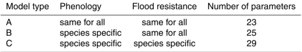
One aim of this study was the analysis of model complexity with regard to model output. Therefore we investigated several model types that differ in complexity regarding the

20

representation of the ecosystem. Since little is known about the ecological parameters in the Kuiseb River, any model would be comparatively simple. We compare three model version of the same area. Table 4 gives an overview about the model differences. In the first model (A) we neglected phenology, all species were evergreen, but dif-fered other traits like maximum transpiration rate. Generally, leaf shed is only partial

25

for all species, thus it suggests itself to neglect seasonal variation. In the second ver-sion B, we included the observed species specific phenology of Camel Thorn and Ana

(17)

HESSD

6, 4155–4207, 2009

models

S. Arnold et al.

Title Page

Tables Figures

◭ ◮

Back Close

Full Screen / Esc

Interactive Discussion Tree (Table 1). For this we added two parameters (l sCam andl sAna), which increased

the degree of complexity (model type B). Finally, in model C, we included more knowl-edge regarding the difference in flood resistance between species, thus allowing the parameterfr_i to be species specific.

In summary, model type C included the most ecological information, strongest

con-5

straints and a mortality that is not only stochastic but also depends on the hydrosystem. In each model application we compared, if the model was able to reproduce the ob-served coexistence of three species. To achieve this goal we parameterized the models accordingly, as pointed out in the next section.

2.6 Parameter sampling

10

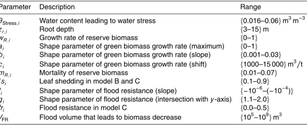
Depending on the model version, the ecological model contained 23–29 parameters. Table 5 gives an overview of those parameters together with their physical range. We used latin hypercube sampling in order to identify parameter sets, which lead to the observed coexistence of three species. This was performed for each model version separately. Only the ecological parameters were calibrated, the hydrological

parame-15

ters were fixed to the values indicated in Table 2.

We constrained the parameter space qualitatively according to the available ecolog-ical information summarized in Table 1: The root depth was largest for Camel Thorn, followed by Ana Tree and Wild Tamarix. Further, we assumed that the growth rate of reserve biomass can be derived from wood density, that is, the larger the wood

den-20

sity the smaller iswR,i. Hence, reserve biomass growth rate was largest for Ana Tree,

followed by Wild Tamarix and Camel Thorn. Additionally, we checked the sampled pa-rameter sets for plausibility: For the shape papa-rametersa_i,b_i, andc_i we allowed only combinations that lead towG,i(t)=0, if

V_WS,i(t)

Rtotal(t−1)≤0 in Eq. (24).

The sampling procedure is illustrated in Fig. 4. For each sampled parameter set (Ωι) 25

we run the model 100 times. We than counted the number of runs, where all three species coexisted and defined the probability of coexistence (P3,ι) for the parameter

(18)

HESSD

6, 4155–4207, 2009

models

S. Arnold et al.

Title Page

Tables Figures

◭ ◮

Back Close

Full Screen / Esc

Interactive Discussion setΩι as follows:

P3,ι(Ωι)=

#B(n=3)

100 , (27)

where #B(n=3) is the number of flood realisations that led to coexistence of all three species. P3,ι gives an indication how robust the modelled coexistence was. If P3,ι is

small, the parameter setΩιonly led to coexistence under very specific flood conditions, 5

while aP₃_,ιnear 1 indicates that the parameter set led to coexistence in almost all flood realisations with the same stochastic properties.

We defined coexistence based on the following criterion: The average reserve biomass during the last 1000 years must exceed the reserve biomass necessary to maintain 10 adult individuals of average size of each species. The method for deriving

10

the number of individuals is described in the Appendix A.

2.7 Analysis of the ensemble models

For analysis of the model results, we used ensemble statistics of hydrological variables of interest and each parameter setΩι (withP3,ι as indicated). The statistics were only

performed on the last 1000 years (2000 time steps) of each simulation, in order to avoid

15

the influence of initial conditions.

The expected ensemble mean for parameter setΩιof the variable of interest (for

ex-ample total ecosystem transpiration) was calculated as follows. We first calculated the time series means of the variable of interest, for each simulation that led to coexistence with the same parameter setΩι. Secondly, we calculated the ensemble mean of the 20

obtained set of time averages.

We only calculated the time average for the subset of η3 simulations, which led to three species coexistence. The statistics was performed on at leastη3=10 simulations. If necessary, additional forward simulations were run in order to obtain 10 simulations

(19)

HESSD

6, 4155–4207, 2009

models

S. Arnold et al.

Title Page

Tables Figures

◭ ◮

Back Close

Full Screen / Esc

Interactive Discussion with coexistence. Each time average of the variable of interest (V_ι,η) is calculated as

Vι,η=

1 2000

t=3000 X

t=1000

Vt, (28)

whereVt is the value of the hydrological variable of interest at time stept, andη the

number of the model realisation. This led to a set ofη3time averages for the variable of interest. Based on this set we calculated the ensemble mean ofη₃realisations, which

5

is

hV_ιi= _η1

3

η₃

X

η=1

V_ι,η. (29)

We proceeded similarly, to obtain the ensemble average of the coefficient of variation of the hydrologic variable. We calculated the dimensionless coefficient of variation (CV_V_ι,η) for the time series:

10

CVV_ι,η =

σ_V_ι,η

Vι,η

, (30)

where σVι,η denotes the standard deviation within the time series of the variable of

interest. Based on this we calculated the ensemble mean ofη3realisations, which is

hCVVιi=

1 η3

η3

X

η=1

CVVι,η. (31)

2.8 Forward simulations with changed flood regime

15

After finding ensembles of suitable parameter sets, we tested how models behaved for changed flood conditions. For this we selected those parameter sets which led to coexistence, and run them again with changed flood regime. We changed the long

(20)

HESSD

6, 4155–4207, 2009

models

S. Arnold et al.

Title Page

Tables Figures

◭ ◮

Back Close

Full Screen / Esc

Interactive Discussion term memory of the flood generation algorithm, by decreasing and increasing the Hurst

exponent (Eq. 18). We grouped the forward simulations into those performed with parameter sets of weak robustness (0.1≤P3,ι≤0.5) and elevated robustness (P3,ι>0.5).

3 Results

Table 6 shows in per cent how many of the 150 000 sampled parameter sets led to

5

P3,ι≥0.1 for models A, B and C. In all cases, the number of parameter sets that

al-lowed for coexistence of all species is very small (less than half percent in all cases). Furthermore, coexistence was modelled for more parameter sets in models A and C, compared to B: The total number of parameter sets leading to P3,ι≥0.1 for model A

and C was about 20 times (both around 0.2%) larger than model B (0.009%, Table 6).

10

Model B was not subject to further investigations because of the low number of param-eter sets leading to three species coexistence.

In Fig. 5 we plotted histograms of the achieved probabilities of coexistence (P3,ι≥0.1)

for model A and C. These histograms give an impression how robust the modelled coexistence was for the different models. The skewnessγof both histograms indicates

15

that most parameter sets showed little robustness (γA=1.5 and γC=1.7). Also, for model A the number of robust parameter sets was larger. For example, consider only parameter sets with 0.1≤P3,ι≤1: In model A 14.3% of those hadP3,ι>0.5, but in model

C only 4.2%.

In order to show how models A and C differ hydrologically we compared the

ensem-20

ble means of hydrologic variables for parameter sets (Ωι) withP3,ι≥0.1. In Fig. 6 we

plotted histograms of the ensemble average of total transpirations (left) and depths to ground water (right). In model A the transpiration was larger (median 161 mm/year) than in model C (median 148 mm/year). In contrast, the depth to ground water was similar for both models (median A: 7.38 m, C: 7.63 m). The difference for model A

25

and C becomes apparent when comparing the extremes of depth to ground water. In model A the ground water was more often modelled close to the surface (0.25

(21)

HESSD

6, 4155–4207, 2009

models

S. Arnold et al.

Title Page

Tables Figures

◭ ◮

Back Close

Full Screen / Esc

Interactive Discussion centile was 5.93 m) than in model C (0.25 percentile was 6.63 m). The opposite is true

for deep ground water tables (0.75 percentile in model A was 11.80 m versus 9.74 m in model C).

In Fig. 7 we plotted histograms of the ensemble means ofCV for total transpiration and depth to ground water. While models A and C differed little with regard to

ensem-5

ble averages of transpiration and depth to ground water, they were much different with regard to the time fluctuations of these variables. In model A the time fluctuation in tran-spiration was much lower (median 0.258) than in model C (0.799). Less pronounced was the difference in the variation of ground water depth, which was also smaller in model A (median 0.025) than in model C (median 0.084).

10

Next, we investigated, if increase in robustness was related to similar parameter sets and similar hydrological conditions. In other words, are all robust parameter sets just small variations of a similar model, or are they completely different? For this, we looked at both the modelled hydrology and the difference between parameters. In Fig. 8 we plotted the medians of transpirations and ground water depth corresponding

15

to the probabilities of coexistence (P3,ι). In Fig. 9 we plotted the medians of CV of

transpiration and ground water depth corresponding to the probabilities of coexistence (P3,ι). Both, Figs. 8 and 9, suggest that in model C a weak relationship exists between

the robustness of the parameter sets (P3,ι) and transpiration (r

2

=0.34) and ground water table (r2=−0.38). Also, a weak relationship exists betweenP3,ι and theCV of 20

transpiration (r2=−0.27) and ground water table (r2=0.14). No such relation exists for model A. Figure 10 gives an impression how robustness of the parameter sets was related to the similarity of four parameters in model C: the root depth (z_r,i), the growth rate of reserve biomass (wR,i), the mortality of reserve biomass (mR,i), and the shape

parameter ci of the conversion rate from reserve to green biomass. The plots show 25

that no relationship between robustness of the parameter sets and parameter similarity existed. The same holds for model A.

In Figs. 11 and 12 we plotted typical time series of the reserve and green biomass, the flood volume and the depth to ground water. These time series allow insight into the

(22)

HESSD

6, 4155–4207, 2009

models

S. Arnold et al.

Title Page

Tables Figures

◭ ◮

Back Close

Full Screen / Esc

Interactive Discussion driving coexistence mechanisms in model A and C. In model C the biomass and ground

water was more affected by the flood (Fig. 12a) than in model A (Fig. 11a). In model C, two alternating states existed. One state was associated with high prevalence of Camel Thorn and Wild Tamarix, small floods and deep ground water table (e.g. year 600–750 in Fig. 12). The other state was associated with high prevalence of Ana Tree and Wild

5

Tamarix, strong floods and shallow ground water table (e.g. year 850–1000 in Fig. 12). In all parameter sets of model C Ana Tree was characterized by a larger vulnerability to flood disturbance than Camel Thorn and Wild Tamarix (Fig. 12b). Model A showed different dynamics. In model A the green biomass and the ground water remained constant after initial fluctuations (Fig. 11). The time series of each species reserve

10

biomass were synchronized with small and frequent disturbances by the flood.

Figure 13 shows how model A and C were affected by a changed long term memory of the flood volume. The relative frequencies refer to the previously identified parameter sets with low robustness (0.1≤P3,ι≤0.5, Fig. 13a) and elevated robustness (P3,ι>0.5,

Fig. 13b). In model C decrease of long term memory decreased species coexistence.

15

This effect was even stronger for the robust parameter sets (Fig. 13b). In model A three species coexistence was little affected by change of the long term memory of the flood, and independent of the robustness of the parameter sets.

4 Discussion

We applied three ecohydrological models that differ in the amount of included

infor-20

mation, and structure. Differences particularly concerned the functional response of the plant species to the hydrosystem along the ephemeral Kuiseb River. We assessed these models regarding their ability to predict coexistence of the three species as was observed in reality. This strategy of pattern-oriented modelling (see e.g. Grimm et al., 2005 and references therein) has been used to model coexistence before. In our study,

25

only two of the three models allow for coexistence of all three species. Further, in both models only few parameter sets reproduce coexistence. This is in line with the classical

(23)

HESSD

6, 4155–4207, 2009

models

S. Arnold et al.

Title Page

Tables Figures

◭ ◮

Back Close

Full Screen / Esc

Interactive Discussion competition models from ecology (e.g. Lotka, 1925; Volterra, 1926) underpinning that

different species can only coexist under the precondition that inter-specific competition (between species) is weaker than intra-specific competition (within the same species). As a result, coexistence can only be found for appropriate parameter combinations that are sparse given the entire parameter space.

5

The comparison between observed and simulated patterns acts as a filter, which allows us to identify, whether a given model structure and parameter combination al-lows coexistence. In this study, only models A and C allow for coexistence. They describe two different coexistence mechanisms for different levels of detail. In model A, species are found to co-exist only, if they have access to different water storages,

10

depending on their root depths (Fig. 11b). Camel Thorn has access to deep ground water and does not compete with any other species. On the other hand, the roots of Ana Tree and Wild Tamarix can only reach the unsaturated layer. Hence, only these two species compete for water in the unsaturated layer. Their coexistence is driven by the trade-offbetween growth rate of reserve biomass (wRi) and water stress (εi), both 15

influencing green biomass and, hence, transpiration demand of the individual species (see Eq. 10). Ana Tree, for instance, has the larger growth rate, but is less water stress resistant. Therefore, coexistence in model A is based on both niche partitioning and trade-offs.

In model B this sensible balance is broken, by introducing the (observed)

phenol-20

ogy. The phenology of Ana Tree in model B reduces the growth period to one season whereas the direct competitor, Wild Tamarix, is evergreen and uses the water resource all year. This provides Wild Tamarix with an advantage in the competition over Ana Tree. In other words, inter-specific competition is enhanced in Model B with the effect that coexistence of all three species is not possible anymore. This is in accordance

25

with the classical competition theory (see above). Note that this also indicates that integrating more knowledge in a model does not automatically lead to more realistic modelling results.

In model C, another coexistence mechanism is enabled, only by allowing for species

(24)

HESSD

6, 4155–4207, 2009

models

S. Arnold et al.

Title Page

Tables Figures

◭ ◮

Back Close

Full Screen / Esc

Interactive Discussion specific vulnerability to the flood. Thus, as opposed to models A and B, the flood has

differential influence both as a water resource and via the destructive impact of the flood; the latter acts directly as an environmental disturbance on the plant species and favours flood resistant species during periods of strong floods. This can compensate the disadvantage of being less competitive than other species in other respects and,

5

hence, can mediate coexistence again. In this case, coexistence results from the com-bination of niche differentiation and environmental disturbance. The latter fits in the context of the Intermediate Disturbance Hypothesis (D’Odorico et al., 2008; Huston, 1979; Grime, 1973; Connell, 1978). The species specific flood resistance in model C allows for ecological differences in the response to disturbance and outbalances too

10

strong advantages from the differences in the phenology, and thus enhances coexis-tence (Roxburgh et al., 2004).

Although both models differ in their structure and coexistence mechanisms, the en-semble statistics of mean hydrologic variables like transpiration and depth to ground water are surprisingly similar between models A and C. (Fig. 6). This is owed to the

15

fact that the hydrological model is the same in both A and C. However, the differences between the two models become apparent, when considering the variation in the time series for both hydrological and ecological variables (depth to ground water, green and reserve biomass) of the system and its sensitivity to environmental change (here: change of the Hurst exponent). The more complex model C shows higher variation

20

in the variables, and is more sensitive to environmental change than model A. This is a logical consequence of the modelled co-existence mechanism. In model C, the flood has both indirect (via the hydrosystem as resource) and direct (as disturbance) impacts on the plant species. Thus, both reserve and green biomass of the different species are independently linked to the flood fluctuations. As a result, species abundances change

25

over time, sometimes with a prevalence of the water conserving species, sometimes with prevalence of the water demanding species. Thus, transpiration and the result-ing ground water level vary accordresult-ingly. In model A, however, the flood influences the ecosystem merely via the reserve biomass (no direct impacts on the green biomass).

(25)

HESSD

6, 4155–4207, 2009

models

S. Arnold et al.

Title Page

Tables Figures

◭ ◮

Back Close

Full Screen / Esc

Interactive Discussion The reserve biomass is able to act as a buffer and to stabilize the entire system (green

biomass, ground water depth).

The results on the influence of the Hurst exponent also give rise to some conclusions on the adequateness of the Intermediate Disturbance Hypothesis (IDH) in ecohydro-logical systems along ephemeral rivers. The IDH primarily argues with the frequency

5

of the disturbance. Our results indicate, however, that the autocorrelation in the vary-ing water supply and so the duration of related disturbance events (cumulative water stress during dry periods, repeated disruptive floods) are crucial for the impact on species coexistence and resilience as well. In this ephemeral ecosystem, consider-ing solely the frequency would reach too short. The importance of autocorrelation/red

10

noise has also been shown in the context of species survival. Schwager et al. (2006) for instance, showed that autocorrelation can be stabilizing or destabilizing depending on the species’ ecological traits.

The results of our study suggest that the assumptions on the functional traits of the species in the plant communities (e.g. regarding resource utilization, flood resistance)

15

and so on the mechanisms of competition/coexistence can influence the modelled hy-drology. Furthermore, ensemble statistics of mean hydrologic variables in this system are driven by the applied hydrological model, whereas the ensemble statistics of fluctu-ations (here: coefficient of variation) is driven by the assumed ecological interactions.

Our forward simulations with different Hurst exponents show that not only the

20

stochasticity of the environmental disturbance (the flood) influences the coexistence of the three species, but also the cyclicity of periods with high and low floods (long term memory, see Sect. 2.3) plays an important role. Most hydrological processes are characterized by long term memory processes (Montanari et al., 1997), which lead par-ticularly in arid regions to extended periods of unusually small or strong events (“Joseph

25

Effect”, Mandelbrot and Wallis, 1968). Our model suggests that this hydrologic charac-teristic might have important influence on ecosystem structure. This finding is in line with other results showing that the fine structure of environmental fluctuations can alter systems dynamics, qualitative trends or ranking orders among scenarios with serious

(26)

HESSD

6, 4155–4207, 2009

models

S. Arnold et al.

Title Page

Tables Figures

◭ ◮

Back Close

Full Screen / Esc

Interactive Discussion implications for management (Frank, 2005; Schwager et al., 2006). Furthermore, the

two models A and C show differences in the sensitivity of species coexistence against a change in the Hurst exponent. While model C reveals a strong sensitivity and a loss of coexistence, model A is found to be rather robust. The reason for this difference is again the buffer capacity of the reserve biomass in absence (model A) and presence

5

(model C) of direct disturbance effects of the flood on the plant species.

The two models A and C can also be interpreted as two types of plant communi-ties which differ in the impact of floods on their species (e.g. indirect only; indirect and direct). But note that both models that successfully modelled coexistence are still ab-stract representations of ecological and hydrological processes along ephemeral rivers.

10

Thus, only limited knowledge of the actual mechanisms is implemented. Such generic models that focus on essential aspects are known to be crucial for integration and analysing consequences of feedback loops when entering new interdisciplinary fields (Baumgartner et al., 2008). This allows formulating new hypotheses, which can then be tested by more complex and structurally realistic models. In our context, additional

15

intra- or interspecific effects might be active in maintaining the observed coexistence. Potentially, a lot more mechanisms can enhance the three species coexistence like random individual effects or multi dimensional tradeoffs (Clark et al., 2007). Thus, our models are just a subset of possible abstraction, which might all reproduce the observed coexistence. In fact it might be impossible to find the “right” model. The

20

co-existence constraint did not limit the possible parameter space enough to lead to a unique ecohydrologic response. However, our models shed light on possible op-tions. They also give hints towards which variables could be measured to increase the understanding about the involved mechanisms.

5 Conclusions

25

The modelling of three species coexistence in a water limited environment is a chal-lenging because feedbacks between ecology and hydrology have to be implemented

(27)

HESSD

6, 4155–4207, 2009

models

S. Arnold et al.

Title Page

Tables Figures

◭ ◮

Back Close

Full Screen / Esc

Interactive Discussion in an appropriate way. The present study introduced a model that facilitates the

in-vestigation of effects of model structure and parameter uncertainty on ecology and hydrology of the water limited system along ephemeral rivers. We applied a range of model versions with a varying degree of included information. Given that only two of three models led to the observed three species coexistence, we conclude that the

5

driving coexistence mechanism is defined by the model structure. On the other hand, the robustness check of the parameter sets leading to three species coexistence indi-cates that the success of the underlying coexistence mechanism is controlled by the combination of the population parameters. Further, depending on the model structure the flood can act as water resource or environmental disturbance or a combination

10

of both. When acting as environmental disturbance the change in long term memory strongly affected the robustness of the parameter sets. Therefore, we conclude that the long term memory of hydrological processes is important in water limited ecosys-tems. In this study, we applied the same hydrological concept for all model versions and only changed the complexity of the ecological model. Considering that the average

15

values of transpiration and ground water table were similar but not their fluctuations, we conclude that the average values of hydrologic variables are mainly controlled by the applied hydrological model, whereas the fluctuations of both are controlled by the applied ecological model.

Our study shows that the species composition in the plant community strongly

in-20

fluences the stability properties of the ecohydrological system (e.g. variation in tran-spiration and ground water depth; variation in reserve and green biomass; sensitivity of species coexistence to change in the Hurst exponent). This stresses the necessity to consider explicitly species composition and functional interactions in the ecosystem when assessing the impact of climate or land use change on water resources and

25

vegetation along ephemeral rivers. This is particularly important in systems where the floods have direct destructive impacts on the vegetation. Here, models are essen-tial that explicitly take into account such disturbance effects (such as model C). The relative importance of the species composition for understanding ecohydrological

(28)

HESSD

6, 4155–4207, 2009

models

S. Arnold et al.

Title Page

Tables Figures

◭ ◮

Back Close

Full Screen / Esc

Interactive Discussion tems, however, came only to light through the subsequent process of changing the

model structure and comparing their outcomes.

Appendix A

Number of individuals

5

The number of adult individuals in population i (NInd,i) was calculated to define the

coexistence criterion for the parameter sampling (Sect. 2.6):

NInd,i =

Ri ∗Aseq R1,i

, (A1)

whereR1,i denotes the reserve biomass of one adult individual of population i. We

simplified the shape of an individual (reserve biomass above and below subsurface) to

10

be a right circular cylinder with maximal trunk radiusr_i, maximal heighthmaxand wood densityρi:

R1,i =π∗ri2∗hmax∗ρi. (A2)

Acknowledgement. We are grateful to Guido van Langenhove, Department of Water Affairs

(DWA), for providing the runoffdata. Further, we thank Joh Henschel, Gobabeb Training and

15

Research Centre, for providing meterologic data and expert knowledge. We also thank to Christoph K ¨ulls and Jens Lange, both from Albert-Ludwigs-University Freiburg, for critical dis-cussion and helpful comments.

References

Arora, V. K. and Boer, G. J.: Simulating competition and coexistence between plant functional

20

types in a dynamic vegetation model, Earth Interact., 10, 1–30, 2006.

Bate, G. C. and Walker, B. H.: Water relations of the vegetation along the Kuiseb River, Namibia, 1991.