Performance of McRAS-AC in the GEOS-5 AGCM: aerosol-cloud-microphysics, precipitation, cloud radiative effects, and circulation

(1)

GMDD

5, 1381–1434, 2012

Performance of McRAS-AC in the

GEOS-5 AGCM

Y. C. Sud et al.

Title Page

Abstract Introduction

Conclusions References

Tables Figures

◭ ◮

Back Close

Full Screen / Esc

Printer-friendly Version Interactive Discussion

Discussion

P

a

per

|

Dis

cussion

P

a

per

|

Discussion

P

a

per

|

Discussio

n

P

a

per

|

Geosci. Model Dev. Discuss., 5, 1381–1434, 2012 www.geosci-model-dev-discuss.net/5/1381/2012/ doi:10.5194/gmdd-5-1381-2012

Geoscientific Model Development Discussions

This discussion paper is/has been under review for the journal Geoscientific Model Development (GMD). Please refer to the corresponding final paper in GMD if available.

Performance of McRAS-AC in the GEOS-5

AGCM: aerosol-cloud-microphysics,

precipitation, cloud radiative e

_ff

ects, and

circulation

Y. C. Sud1, D. Lee1,2,3, L. Oreopoulos1, D. Barahona1,4, A. Nenes5, and M. J. Suarez1

1

NASA Goddard Space Flight Center, Greenbelt, MD, USA 2

Universities Space Research Association, Columbia, MD, USA 3

Seoul National University, Seoul, South Korea 4

I.M. Systems Group Inc., Rockville, Maryland, USA 5

School of Atmospheric and Earth Science, Georgia Tech. Atlanta, Georgia, USA

Received: 11 May 2012 – Accepted: 21 May 2012 – Published: 8 June 2012

Correspondence to: Y. C. Sud (yogesh.c.sud@nasa.gov)

(2)

GMDD

5, 1381–1434, 2012

GEOS-5 AGCM

Y. C. Sud et al.

Title Page

Tables Figures

◭ ◮

Back Close

Full Screen / Esc

Discussion

P

a

per

|

Dis

cussion

P

a

per

|

Discussion

P

a

per

|

Discussio

n

P

a

per

|

Abstract

A revised version of the Microphysics of clouds with Relaxed Arakawa-Schubert and Aerosol-Cloud interaction scheme (McRAS-AC) including, among others, the Barahona and Nenes ice nucleation parameterization, is implemented in the GEOS-5 AGCM. Various fields from a 10-yr long integration of the AGCM with McRAS-AC were

com-5

pared with their counterparts from an integration of the baseline GEOS-5 AGCM using satellite data as observations. Generally McRAS-AC simulations have smaller biases in cloud fields and cloud radiative effects over most of the regions of the Earth than the baseline GEOS-5 AGCM. Two systematic biases are identified in the McRAS-AC runs: one under-prediction of cloud particles around 40◦_S–60◦_{S, and one over-prediction of} 10

cloud water path during Northern Hemisphere summer over the Gulf Stream and North Pacific. Sensitivity analyses show that these biases potentially originate from biases in the aerosol input. The first bias is largely eliminated in a sensitivity test using 50 % smaller sea-salt aerosol particles, while the second bias is much reduced when inter-active aerosol chemistry was turned on. The main drawback of McRAS-AC is dearth of

15

low-level marine stratus clouds, probably due to lack of boundary-layer clouds that is an outcome of explicit dry-convection not yet implemented into the cloud model. Nev-ertheless, McRAS-AC simulates realistic clouds and their optical properties that can further improve with better aerosol-input. Thereby, McRAS-AC has the potential to be a valuable tool for climate modeling research because of its superior simulation

capa-20

bilities that physically couple aerosols, cloud microphysics, cloud macrophysics, and cloud-radiation interaction for all clouds.

1 Introduction

Traditionally, meteorologists focused on severe weather and precipitation forecasts and much less attention was paid to cloud water. There are two reasons for this. First,

in-25

(3)

GMDD

5, 1381–1434, 2012

GEOS-5 AGCM

Y. C. Sud et al.

Title Page

Tables Figures

◭ ◮

Back Close

Full Screen / Esc

Discussion

P

a

per

|

Dis

cussion

P

a

per

|

Discussion

P

a

per

|

Discussio

n

P

a

per

|

episode; second, weather forecast is useful for a week (or less), which is too short for cloudiness and its radiative e_ffects to exert much influence on the synoptic weather systems. Consequently, ad hoc ways to assess cloud radiative forcing were deemed sufficient. However, once the emphasis of forecasting turned to climate, radiative forc-ings and everything that a_ffects them including influence of aerosols on clouds, cloud

5

radiative effects (CRE), and greenhouse gases become very important. Among them, cloud-aerosol interaction (Andreae and Rosenfeld, 2008) is in early stages of devel-opment, but the progress is rapid (e.g., Quaas et al., 2004; Roelofs et al., 2006; Sud and Lee, 2007; Morrison and Gettelman 2008; Stevens and Feingold, 2009; Liu et al., 2011). Toward this goal, we have recently revised and updated an aerosol-cloud

10

interaction (AC) module of the well-performing McRAS (Microphysics of clouds with

RelaxedArakawa-Schubert) cloud scheme. This manuscript presents the implementa-tion and evaluaimplementa-tion of McRAS-AC in the GEOS-5 AGCM.

The pioneering works of Gibbs (1876, 1878), and K ¨ohler (1936) laid the foundation of cloud droplet formation; combined with the dynamics of supersaturation generated

15

from existing droplets (e.g., Nenes et al., 2001) or cloud ice particles leads to physically-based aerosol activation parameterizations for GCMs (e.g., Abdul-Razzak and Ghan 2000, 2002; Nenes and Seinfield, 2003; Liu and Penner, 2005; Barahona and Nenes, 2009a, b; Ghan et al., 2011). More aerosols increase the number density of cloud particles (CP) (Twomey, 1977; Seinfeld and Pandis, 1996) and thereby suppress

au-20

toconversion and accretion that form precipitating hydrometeors (e.g., Albrecht, 1989; Seifert and Beheng, 2001, 2006). We cite a few recent studies that show the impact of aerosols on (i) weather and climate prediction (Lohmann, 2006; Kim et al., 2006; Krishnamurti et al., 2009; Sud et al., 2009; Wilcox et al., 2009; Lau et al., 2009) made with an earlier version of McRAS-AC using Liu and Penner (2005) IN parameterization;

25

(4)

GMDD

5, 1381–1434, 2012

GEOS-5 AGCM

Y. C. Sud et al.

Title Page

Tables Figures

◭ ◮

Back Close

Full Screen / Esc

Discussion

P

a

per

|

Dis

cussion

P

a

per

|

Discussion

P

a

per

|

Discussio

n

P

a

per

|

affecting the Indian monsoons (Lau and Kim, 2007); and (vi) freezing of in-cloud drops with release of latent heat of freezing (Rosenfeld et al., 2000, 2006). The debate on how and/or how much do aerosols influence different clouds to foster or suppress pre-cipitation yield from different cloud types continues (e.g., Gunturu, 2010; Li et al., 2011; Lance et al., 2011; Koren et al., 2012). An outcome of increasing cloud particle

num-5

ber concentrations (CPNC) is the accompanying reduction in cloud particle sizes in the distribution. It slows the autoconversion and accretion of cloud drops to form precipi-tation size hydrometeors and that gives liquid cloud particles and embryonic raindrops the time to ascend in the convective updrafts and glaciate at subfreezing temperatures to release latent heat of freezing that in turn augments the cloud buoyancy. How this

10

manifests in convective clouds, depends upon how much further the convective towers ascend and how much additional condensate and precipitation is generated. These in turn depend on the local atmospheric sounding.

Numerical models can simulate all of the above processes, if the cloud-physics pa-rameterizations allows for them and the ambient aerosol fields are reasonably

accu-15

rate. However, many GCMs still obtain clouds invoking a number of simplifying and/or ad hoc assumptions (Bacmeister et al., 2006; Randall, 2010) that often ignore the aerosol effects on clouds. At the present time, even understanding of the climatic impact of aerosols remains uncertain (IPCC, 2007), while most present-day climate modelers have started to include prognostic parameterizations of the direct and

in-20

direct aerosol effects in the cloud schemes and intercompare their performance with other models (Bellouin et al., 2011). Several complexities and uncertainties still con-found cloud modelers. For example, aerosol input, implying aerosol size distribution and speciation and their hygroscopic properties, and their activation/nucleation poten-tial to become CCN/IN must be inferred from aerosol chemistry which is also

uncer-25

(5)

GMDD

5, 1381–1434, 2012

GEOS-5 AGCM

Y. C. Sud et al.

Title Page

Tables Figures

◭ ◮

Back Close

Full Screen / Esc

Discussion

P

a

per

|

Dis

cussion

P

a

per

|

Discussion

P

a

per

|

Discussio

n

P

a

per

|

typical climate model. Without the key microphysical and dynamical feedbacks, the benefit of including aerosol-cloud interactions in GCMs becomes limited as the sensi-tivity of cloud properties to aerosol gets strongly biased (Stevens and Feingold, 2009). Its importance was also evidenced in cloud seeding experiments, as summarized by Cotton and Pielke (1995). They state that there is a limited window of opportunity, and

5

cloud seeding becomes a hit or miss venture and its full potential is not realized. One infers that to make a verifiable impact on climate, the atmospheric aerosols too must be known reasonably well at the cloud-scale.

We also need a cloud scheme that estimates sub-grid scale mass flux and fractional cloud cover (for both convective and large-scale clouds), their buoyancy induced

up-10

draft and the rain-evaporation induced convective downdrafts. Another requirement is that the model can perform level-by-level entrainment and detrainment of the ambi-ent air mass with grid-scale vertical velocity, humidity, aerosols (different species, their mass, and number concentrations), as well as existing clouds (water substance mass and particle number concentrations) and mix them with the in-cloud vertical velocity

15

and temperatures to determine the CCN/IN needed for condensation/deposition. With calculations to yield the time to ascend through the model-layer, the cloud model can perform precipitation microphysics on the best possible physics for simulating the influ-ence of interactive aerosols on clouds. In Sect. 2.2, we will highlight how McRAS has the unique ability to provide cloud-scale processes described above. Subsequent to

20

including the aerosol cloud interaction, McRAS is renamed McRAS-AC. The question we want to answer is whether McRAS-AC is a worthwhile option to simulate the cloud optical properties and climate with the GEOS-5 GCM.

Mixed phase clouds are among the most challenging features to simulate in GCMs. Ultimately, the goal is a realistic prediction of mixed phase water and ice mass

frac-25

(6)

GMDD

5, 1381–1434, 2012

GEOS-5 AGCM

Y. C. Sud et al.

Title Page

Tables Figures

◭ ◮

Back Close

Full Screen / Esc

Discussion

P

a

per

|

Dis

cussion

P

a

per

|

Discussion

P

a

per

|

Discussio

n

P

a

per

|

Bergeron-Findeisen process (Bergeron, 1935) in the following manner. At subfreezing temperatures, the vapor pressure di_fferences over cloud water and ice particles are large enough to create substantial vapor pressure gradient between them to induce mass transfer of cloud cloud-water to cloud-ice through the intervening atmosphere. Simultaneously, precipitating hydrometeors collect cloud water/ice particles during fall

5

through the cloud (sometimes even from clear air if it happens to be supersaturated with respect to the ice). In this way, precipitation removes cloud particle mass and re-duces the in-cloud CPNC. Altogether, these processes add up to make the sink term of CPs for which each of the components must be parameterized. The sum of source and sink terms yields the time rate of change of mass and number concentration as shown

10

in the mass and CP number budget equations of Morrison and Gettelman (2008). To close the system, one also needs a precipitation microphysics scheme. Thus an end-to-end aerosol-cloud interaction parameterization starts with aerosols activating as CCN and/or IN to receive condensation and/or ice deposition or nucleate cloud wa-ter through contact or immersion nucleation; needs a reasonable treatment of mass

15

transfers among liquid, ice and vapor phases of cloud water with precipitation micro-physics for liquid and ice clouds. Section 2 gives a brief description of GEOS-5 AGCM hosting McRAS-AC as one of its options. Section 3 gives the simulation experiments. Section 4 gives simulation results and key biases. Section 5 has summary and conclu-sions and some research directions to make McRAS-AC simulations more realistic.

20

2 Cloud schemes: GEOS-5 GCM and McRAS-AC

2.1 GEOS-5 GCM

The Fortuna 2.5 version of the GEOS-5 GCM is documented by Molod et al. (2012); it describes the model performance with several new updates to the earlier MERRA version (Rienecker et al., 2008). Briefly, it employs the Relaxed Arakawa-Schubert

25

(7)

GMDD

5, 1381–1434, 2012

GEOS-5 AGCM

Y. C. Sud et al.

Title Page

Tables Figures

◭ ◮

Back Close

Full Screen / Esc

Discussion

P

a

per

|

Dis

cussion

P

a

per

|

Discussion

P

a

per

|

Discussio

n

P

a

per

|

water for cloud microphysics. RAS produces prognostic cloud cover, diagnostic cloud ice and cloud water mixing ratios, and cloud water. Other upgrades comprise of large-scale condensation and evaporation, auto-conversion and accretion of cloud water and ice, sedimentation of cloud-ice, and re-evaporation of falling precipitation following Bacmeister et al. (2006). Its long-wave radiative transfer calculations are due to Chou

5

et al. (2001), and its shortwave radiative transfers are due to Chou and Suarez (1999). These handle interactions with simulated clouds, cloud water, water vapor, and exter-nally prescribed trace gases. In addition, shortwave calculation includes absorption, scattering and transmission by aerosols, i.e., it treats the direct effect of aerosols only. For more details, refer to Molod et al. (2012) and Rienecker et al. (2008). We will refer

10

to the GEOS-5 AGCM as baseline model and/or AGCM.

2.2 McRAS-AC

The latest version of McRAS (Sud and Walker, 2003a) is chosen as the cloud scheme for including the aerosol-cloud interactions. Its evolution dates back to development of McRAS built from RAS moist convection. Initially, McRAS used cloud microphysics

15

based on the work of Sundqvist (1988) and Tiedtke (1993) along with other upgrades namely rain-evaporation (Sud and Molod, 1988) and convective downdrafts (Sud and Walker, 1993). It is extensively evaluated in several Single Column Model intercom-parisons (e.g., Ghan et al., 2000; Xie et al., 2002; Xu et al., 2005; Klein et al., 2009; Morrison et al., 2009). Its climate simulations with GEOS-2 GCM (Sud and Walker,

20

1999b) were more realistic than that of the baseline GEOS-2 model. It produced reasonable intra-seasonal oscillations (ISO) in GEOS-2 and GEOS-3 AGCMs. The ISOs were also well reproduced in the NCAR implementation of McRAS (Maloney and Hartmann, 2001). Nevertheless, these applications also highlighted some weak-nesses that were addressed in subsequent upgrades (Sud and Walker, 2003a, b).

25

(8)

GMDD

5, 1381–1434, 2012

GEOS-5 AGCM

Y. C. Sud et al.

Title Page

Tables Figures

◭ ◮

Back Close

Full Screen / Esc

Discussion

P

a

per

|

Dis

cussion

P

a

per

|

Discussion

P

a

per

|

Discussio

n

P

a

per

|

were assumed for land and ocean following Del Genio et al. (1996), while the volume and effective radii of CPs were estimated from another set of empirical assumptions (Sud and Walker, 1999a).

The current aerosol-cloud interaction microphysics modules are documented in Sud and Lee (2007). The new addition is the ability to use Barahona and Nenes (2009a) as

5

an alternative to Liu and Penner (2005) aerosol nucleation (IN). The version of McRAS-AC used herein has McRAS cloud-scheme plus Fountoukis and Nenes (2005) aerosol activation parameterization to yield CCN and Barahona and Nenes (2009a) scheme for ice nucleation. For precipitation microphysics, Sud and Lee (2007) is used for liquid and Sundqvist (1988) scheme is used for mixed and ice phase clouds. In-cloud evaporation

10

and/or precipitation and self collection of cloud water are parameterized by Sud and Lee (2007), which is a recast of Seifert and Beheng (2001, 2006) to obtain relations for thicker clouds encountered in a coarse resolution GCM. Any change in cloud mass by condensation/deposition and subsequent removal by precipitation, works interactively through an implicit backward numerical integration that approximates the solution of

15

the coupled nonlinear differential equations that are otherwise impossible to solve with-out iteration. Lacking an IPNC-based snow precipitation scheme, McRAS-AC currently uses the Sundqvist (1988) parameterization for mixed phase and ice phase precipi-tation. However, inclusion of ice nucleation (IN) (Barahona and Nenes, 2009a, b) and Bergeron-Findeisen cloud water-to-ice mass transfer (Rotstayn et al., 2000) cloud

liq-20

uid and ice mass fractions and corresponding CPNC (LPNC plus IPNC) are calculated consistently to conserve mass and IPNC budgets. Nevertheless, CPNC reduction by precipitation is non-linear and is based on a curve-fitted relationship between cloud mass and number concentration for the prescribed Gamma distribution of cloud parti-cle sizes. Homogenous freezing of in-cloud water drops surviving up to−38◦C or even

25

(9)

GMDD

5, 1381–1434, 2012

GEOS-5 AGCM

Y. C. Sud et al.

Title Page

Tables Figures

◭ ◮

Back Close

Full Screen / Esc

Discussion

P

a

per

|

Dis

cussion

P

a

per

|

Discussion

P

a

per

|

Discussio

n

P

a

per

|

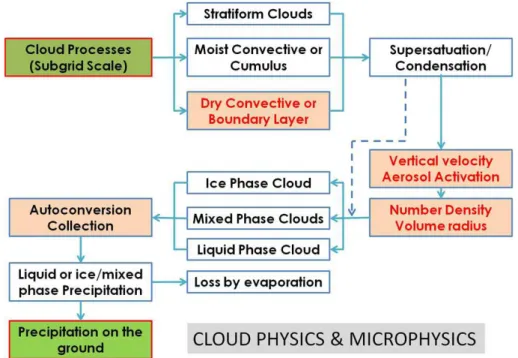
through a block diagram shown in Fig. 1. It shows how aerosol activation by vertical ascent or its equivalent cooling create condensate, CCN and/or IN while cloud-scale microphysics creates precipitation and reduce CPNC. McRAS-AC is implemented as an option to work with the baseline GEOS-5 GCM.

3 Simulation experiments

5

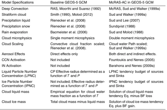
We performed two 10-yr long simulations, one with the baseline Fortuna 2.5 version of the GEOS-5 AGCM (referred to as baseline) with its own cloud scheme and one with the same GEOS-5 AGCM, but for the newly implemented McRAS-AC cloud physics module as an option for handling the moist processes in the AGCM. Table 1 shows key differences between schemes. In the GEOS-5 implementation, the explicit dry

10

convection-based treatment of McRAS-AC (Sud et al., 2009) eddy transport draws the near surface water vapor to the level of neutral buoyancy somewhere near the PBL top; thereby, it raises the height of the cloud base and dries the boundary layer. However, in the present implementation, McRAS-AC relies on the PBL scheme of the baseline model. The monthly climatology of aerosols is taken from GOCART (Chin et al., 2002)

15

and is based on extensive aerosol model development and calibration/validation exer-cises (Colarco et al., 2010). Currently we use five externally mixed aerosols namely sulfates, sea-salt, mineral dust, black carbon and organic carbon. GOCART provides the time dependent mass distributions of each aerosol species, from which the aerosol number is calculated by making separate sectionals of aerosol sizes, called modes.

20

(10)

GMDD

5, 1381–1434, 2012

GEOS-5 AGCM

Y. C. Sud et al.

Title Page

Tables Figures

◭ ◮

Back Close

Full Screen / Esc

Discussion

P

a

per

|

Dis

cussion

P

a

per

|

Discussion

P

a

per

|

Discussio

n

P

a

per

|

4 Results

A comparison of two 10 year integrations, one withMcRAS-ACin the GEOS-5 AGCM (hereafter referred to as “MAC”) and one with the baseline GEOS-5 AGCM (hereafter, referred to as “CTL”) are used to examine precipitation, clouds, their water paths, ef-fective radii, and CREs. There are two aspects of this intercomparison; one is the

5

differences due to cloud parameterization schemes, in CTL and MAC, the other is the influence of aerosol activation and associated cloud particle numbers and sizes; how-ever, the effective radii of cloud liquid and ice particles are empirically prescribed in CTL runs as functions of temperature and cloud water path. The two most intractable com-ponents of the simulated climate change are the CREs and how these would change

10

with any climate change scenario. GCMs need to simulate realistic (implying as much bias free as possible) CREs. The goal here is to determine how MAC and CTL cli-matologies compare with each other and how well they hold up against observations. Can they simulate the annual cycle reasonably well, and, how much can these be trusted to simulate realistic climate change scenarios? Specifically the aim is to

de-15

termine MAC seasonal climatology and its biases and thereafter design upgrades to ameliorate them. Second, are there reasonable sensitivities to aerosol mass and num-ber concentration of the real environment, and can they be used to improve model’s CREs and understand the influence of aerosols on clouds, and cloud-radiation interac-tions and its consequences on the regional climate change? We produced MAC and

20

CTL seasonal average fields for DJF, MAM, JJA, SON and an annual mean for several key fields. However, to keep the number of figures reasonable for the reader, we show only the climatology of the two extreme seasons, DJF and JJA, and the annual means. Although revising the algorithms and making aerosol input modifications to ameliorate some of the biases are left for Part 2 of the paper; we include two test runs showing

25

(11)

GMDD

5, 1381–1434, 2012

GEOS-5 AGCM

Y. C. Sud et al.

Title Page

Tables Figures

◭ ◮

Back Close

Full Screen / Esc

Discussion

P

a

per

|

Dis

cussion

P

a

per

|

Discussion

P

a

per

|

Discussio

n

P

a

per

|

4.1 Precipitation fields

The left two panels of Fig. 2 depict the broad feature of rainfall climatology of MAC and CTL. Both model-simulations have reasonable ITCZ and SPCZ, with intense convective rainfall, as expected. In DJF large rainfall is simulated over the South American land-mass, Australia, the tropical islands of Southeast Asia, over the North Atlantic along

5

the eastern boundary of Asia, and over the Gulf Stream along the eastern boundary of North America. Large rainfall also occurs over the rising branch of Ferrell cell between 40◦_S–60◦_{S. In JJA, we see tropical rain including the ITCZ at its northward location.}

The simulated tropical Pacific ITCZ is somewhat weaker with less than observed rain-fall intensities in the mid-span of the Pacific ITCZ band and somewhat more than the

10

observed near and over the land masses at both ends of the ITCZ band, presum-ably due to orographic intensification of precipitation; thus more water vapor converges on to land away from its natural location(s) over the tropical Pacific Ocean where the model simulated climatology has a rainfall deficit. Indian and Asian regions have real-istic monsoons and associated rainfall. Northwards of Sahel, the Sahara desert is dry

15

in JJA as it should be. Generally, MAC and CTL biases in precipitation are quite simi-lar to each other, although MAC does better on the RMSE scores in DJF and JJA but not on ANN (see Table 3). The majority of the biases are associated with orographic intensification of precipitation and its related moisture convergences; it is a proverbial problem with a number of numerical models. According to Chao (2012), the problem

20

is largely solved in his GEOS-5 AGCM runs, but the Chao-code has not been imple-mented in the Fortuna 2.5 version of GEOS-5 AGCM. Excessive rainfall biases along southern Andes, hilly regions of South Africa, and tropical islands of south East Asia is seen in DJF. Precipitation biases around eastern regions of Himalayas, and Andes through South and Central America (redder regions in the difference maps, Fig. 2)

25

(12)

GMDD

5, 1381–1434, 2012

GEOS-5 AGCM

Y. C. Sud et al.

Title Page

Tables Figures

◭ ◮

Back Close

Full Screen / Esc

Discussion

P

a

per

|

Dis

cussion

P

a

per

|

Discussion

P

a

per

|

Discussio

n

P

a

per

|

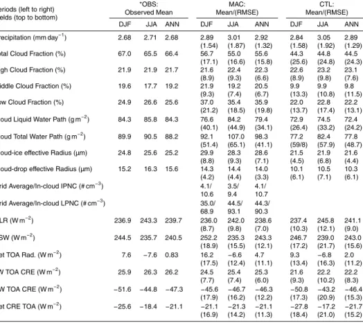
MAC minus OBS means that the corresponding biases are lesser in MAC. Overall, both simulations, MAC and CTL, do reasonably well in comparison to GPCP precipita-tion data (Adler et al., 2003). In the boreal winter (DJF) season, MAC (CTL) simulate global mean precipitation of 2.89 (2.84) mm day−1_{versus the somewhat smaller value}

of 2.68 mm day−1 _{in the GPCP data. The corresponding boreal summer (JJA) values} 5

are 3.01 (3.04) mm day−1_{versus 2.71 mm/day in the GPCP data. Indeed, the simulated}

precipitation values are consistent with global mean surface evaporation. Accordingly, global condensation heating of McRAS-AC are 6.0 (8.7) W m−2_{too large in DJF (JJA).}

Since SSTs are prescribed, excessive evaporation over the oceans can occur without any negative feedback that could reduce the SSTs and evaporation. (See Table 3 for

10

the details).

DJF averages in the tropics show that the MAC (CTL) rainfall distribution over the sharp ITCZ is less (more) intense than the corresponding GPCP data. However, MAC simulations make up for the reduction with small increases over the neighboring grid cells north and south of the ITCZ. The orographic rainfall intensification biases are

15

consistently positive and quite similar in both MAC and CTL simulations. Clearly, the AGCM has a problem reproducing observed precipitation with flow across the steep hills; this is a persistent bias in the GEOS-5 GCM. Bangert et al. (2011) suggest use of orographic uplift as a “pseudo-updraft velocity” superposed on the vertical velocity normally resolved by the model as a solution but we have not experimented with it.

20

For JJA, both MAC and CTL simulate the Equatorial Pacific ITCZ in the middle of its east-west span is weak similarly, even though CTL simulation has a slightly better organized ITCZ. On the whole, both cloud schemes show persistent biases that need some attention (Fig. 2, two right panels).

Indeed, statistically significant differences are important. When this is done with each

25

(13)

GMDD

5, 1381–1434, 2012

GEOS-5 AGCM

Y. C. Sud et al.

Title Page

Tables Figures

◭ ◮

Back Close

Full Screen / Esc

Discussion

P

a

per

|

Dis

cussion

P

a

per

|

Discussion

P

a

per

|

Discussio

n

P

a

per

|

East Pacific in DJA and mid Pacific in JJA; some differences are significant over the tropical Atlantic and Indian Ocean in both seasons. In these convergence zones MAC precipitation is less than that of CTL. Naturally, areas of statistical significance on an-nual mean fields are even smaller in conformity with our understanding that biases often reduce by averaging not only over the annual cycle but also across space and

5

multi-model ensembles even over shorter time periods. Overall, the rainfall differences between MAC and CTL in a 2-tailed student t-test at 95 % significance are small and without much structure except for ice-covered Polar Regions. Thus both schemes pro-duce similar rainfall fields with very similar biases (vis- `a-vis the GPCP data) barring the biases introduced by orographic intensification which are truly large.

10

4.2 Cloud fractions and water path

Cloud fractions and in-cloud water particle number concentration and water path are three quantities that govern the CREs (Sect. 4.4.2); biases in the radiation fields of the shortwave and longwave radiation can be attributed to biases in cloud fraction and cloud water path and e_ffective radius of cloud particles. The vertical alignment of clouds

15

(Oreopoulos et al., 2012) or the prescribed cloud water-path also influences the CREs. These are discussed at length in the subsections of Sect. 4.4

4.2.1 Cloud fractions

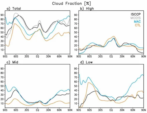
Figure 4 shows yearly averaged zonal mean cloud fractions for the atmospheric column as a whole. The total cloud fraction is further divided into three sections: high, middle,

20

and low level values and their biases and RMSE with respect to ISCCP data (Rossow and Schi_ffer, 1999) for DJF, JJA and annual means (Table 3). The simulated total cloud fractions of MAC are larger than those of CTL but less than the observed. Its zonal distribution tracks the observed quite well. In comparison, column averaged cloud frac-tion biases in CTL are negative when averaged globally. Whereas MAC biases are also

25

(14)

GMDD

5, 1381–1434, 2012

GEOS-5 AGCM

Y. C. Sud et al.

Title Page

Tables Figures

◭ ◮

Back Close

Full Screen / Esc

Discussion

P

a

per

|

Dis

cussion

P

a

per

|

Discussion

P

a

per

|

Discussio

n

P

a

per

|

the tropics. Overall, MAC simulations produce lesser biases than the CTL. If the sim-ulated cloud fractions are far off, the only way to get reasonable CRE is to tune cloud water or scaling the cloud fraction and/or their optical properties; while MAC uses cloud water path scaling, CTL performs convective cloud fraction scaling (shown in Table 1). Moreover, CTL total clouds are consistently less than observed; MAC total clouds are

5

similar to CTL in the tropics but larger than CTL in the higher latitudes (Fig. 4a) and get even more than the observed in Polar Regions, a bias that has been highlighted before. Further details of high, middle, and low level clouds are as follows.

High clouds (above 400 hPa) are equally robust and realistic in both CTL and MAC simulations except for the Polar Regions, where MAC high clouds show larger biases

10

than the CTL (Fig. 4b). On seasonal time-scales the biases do look quite di_fferent. Some biases of less than observed high cloud over north of India and western United States, and Argentina are common to both MAC and CTL simulations in DJF as well as JJA (not shown) leading to discernible signatures in the annual averages. Over the oceans, MAC does better than CTL, which overestimates high clouds. However, high

15

clouds are more than observed in both MAC and CTL simulations in both DJF and JJA seasons. In DJF, MAC (CTL) simulates about−0.3 % (0.7 %) bias in the observed high

clouds fraction of about 22 %. In JJA too both MAC (CTL) simulate 0.5 % (1.3 %) more high clouds and those biases are reasonable for GCM applications. Perhaps RAS, the convective scheme of both the CTL and MAC cloud schemes is responsible for the

20

similarity of high cloud fractions in the tropics. A word of caution about ISSCP data is warranted here. ISSCP retrieval algorithm is unable to detect very thin cirrus; therefore its own bias is towards less than the actual deep clouds and that could explain, in part, the high cloud biases as a spurious model deficiency.

The middle level clouds, 700–400 hPa, are considerably better in MAC vis- `a-vis CTL

25

(15)

GMDD

5, 1381–1434, 2012

GEOS-5 AGCM

Y. C. Sud et al.

Title Page

Tables Figures

◭ ◮

Back Close

Full Screen / Esc

Discussion

P

a

per

|

Dis

cussion

P

a

per

|

Discussion

P

a

per

|

Discussio

n

P

a

per

|

in MAC started producing more mid-level clouds after melting of snowfall at 0◦_{C was}

introduced (Sud and Walker, 2003b). In the tropics, the snow melts at around 500hPa, produces an inversion and that debars cumulus towers from penetrating through it. We also point out that mid-level cloud fractions in the ISSCP data may be too large (Chen and Del Genio, 2008). Moreover, the mid-level cloud percentages are almost same as

5

high cloud percentages, but for now MAC simulates them and our radiation balances suggest that cumulus congestus and mid-level detrainment by high latitude cumulus clouds may be reasonable (Johnson et al., 1999); however, the fall velocity of embry-onic hydrometeors soon after autoconversion, is chosen to yield optimal estimates of cloud water (Sud and Lee, 2007). Even though both large-scale schemes (i.e., MAC

10

and CTL) use Slingo and Ritter (1985) type of critical relative humidity dependence for the emergence of stratiform clouds, the McRAS-AC determines only its tendency and not the amount (Sud and Walker, 1999a) as well as employs moist convection asso-ciated with stratiform clouds as an additional upgrade (Sud and Walker, 2003b). The latter would tend to increase the cloud fraction and its vertical correlation that shows

15

up in the CRE analysis of Oreopoulos et al. (2012).

On low level clouds (surface to 700 hPa), MAC simulation is better than CTL between 30◦_{S to 30}◦_{N, but at higher latitudes MAC shows large biases particularly in the}

Po-lar Regions, where observations are not so reliable. Regardless, this makes low level cloud fractions of MAC somewhat inferior. The biases at high latitudes occur in all the

20

seasons as well as the annual means. CTL simulations produce less than observed low-level clouds, but they get better at higher latitudes (Fig. 4d). MAC simulates almost 50 % more low level clouds at high latitude regions. Corresponding high latitude biases in the CTL are only half as much. Overall, CTL simulated PBL clouds are about 4 % less than the observed. However, in the tropics, MAC simulation is still as good as

25

(16)

GMDD

5, 1381–1434, 2012

GEOS-5 AGCM

Y. C. Sud et al.

Title Page

Tables Figures

◭ ◮

Back Close

Full Screen / Esc

Discussion

P

a

per

|

Dis

cussion

P

a

per

|

Discussion

P

a

per

|

Discussio

n

P

a

per

|

perform this function. Evidently, there is a need to revitalize the explicit dry convection. In the regions of moist convection, moisture is transported to the top of the PBL through convective transport, but at high latitude with much less surface fluxes, dry convection is initiated by the diurnal cycle of surface temperature. Only if the PBL convective eddy gets saturates, it detrains a fractional PBL-cloud, which dissipates via cloud

munch-5

ing and cloud top entrainment instability (CTEI). Moreover, precipitation in the Polar Regions often emerges as tiny snow particles from the ice fog falling out of clear sky (diamond dust; Greenler, 1999). McRAS-AC, may be earmarking such layers as cloudy because local RH of the ambient atmosphere exceeds the saturation vapor pressure of ice (criteria used to identify a large-scale cloud). These ideas can be formulated as

10

algorithms that can mitigate the high latitude cloud biases of McRAS reflecting in MAC simulations.

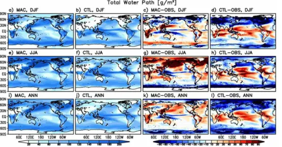
4.2.2 Total cloud water path

The geographical distribution of total cloud water path (=sum of liquid plus ice water paths) simulated by MAC and CTL are shown in Fig. 5. First, CTL biases are

consis-15

tently negative in the high latitude regions and positive in the tropics. Despites more cloud water in the tropics, positive biases in the tropics are not able to cancel out the high latitude negative biases (see Table 3 for means and RMSEs). However, since the effective radii of cloud drops are prescribed in CTL, it decouples the cloud mass and number density from the cloud water budget. The MAC simulation also shows such

20

biases and allows the modeler to optimize the results by tuning the disposable param-eters. MAC RMSEs are similar to those of CTL whereas its biases are better connected with the cloud water path. Too high total and liquid cloud water path is due to high water content in the storm tracks along the eastern boundary of Asia and North America fol-lowing the North Pacific Currents and the Gulf Stream. This bias is so strong in the JJA

25

(17)

GMDD

5, 1381–1434, 2012

GEOS-5 AGCM

Y. C. Sud et al.

Title Page

Tables Figures

◭ ◮

Back Close

Full Screen / Esc

Discussion

P

a

per

|

Dis

cussion

P

a

per

|

Discussion

P

a

per

|

Discussio

n

P

a

per

|

stratus clouds near the west coast of North and South America. A worthwhile strategy is needed to address them with additional cloud physics upgrades.

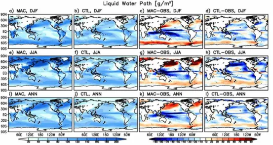
4.2.3 Liquid cloud water path

The simulated liquid cloud water path is shown in Fig. 6. Here, SSM/I dataset is from Weng et al. (1997), which contain data over oceans. This has a distinctly different

pat-5

tern than the total water path. Its mean statistics are better for MAC than CTL, while its RMSEs are not. Evidently, MAC under predicts cloud water path in the ITCZ, SPCZ in the DJF, JJA and ANN averages. Once that happens, both mass and number densi-ties of cloud water adjust proportionally. Moreover, our analysis of fractional cloudiness shows that low level cloud fractions are more than the observed; therefore large

wa-10

ter content in the stratiform regime and less particle numbers may have contributed to this bias. However, readjusting the disposable (tunable) parameters of the scheme can potentially ameliorate this problem. On other specifics, there is too much liquid as well as total water in the 40–60◦_{S region of roaring winds in DJF. In fact, as the total cloud}

water bias reverses in JJA while the liquid cloud water still has a positive bias, we infer

15

that the ice amount over the region in JJA gets too small and that points to lack of IN and a delayed Bergeron process which must wait to kick in until sufficient IN are avail-able for water vapor to deposit on. This may well be related to lack of ice nucleating aerosols. Since ice is also an absorber of solar radiation, lack of ice in the clouds near the boundary-layer may be one of the causes for the bias in solar absorption, which can

20

only appear in DJF because the solar radiation at 40–60◦_{S latitudes is much smaller}

in JJA. Low cloud water path offthe west coast of Americas in JJA is to be expected lacking the boundary layer stratus and that indeed happens in both MAC and CTL sim-ulations. The liquid water content in the storm track regions of Asia and east coast of North America (over the nearby ocean) has strong positive (negative) bias for MAC

25

(18)

GMDD

5, 1381–1434, 2012

GEOS-5 AGCM

Y. C. Sud et al.

Title Page

Tables Figures

◭ ◮

Back Close

Full Screen / Esc

Discussion

P

a

per

|

Dis

cussion

P

a

per

|

Discussion

P

a

per

|

Discussio

n

P

a

per

|

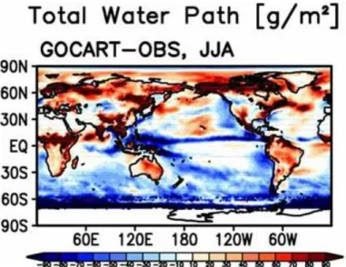
an under prediction of precipitation rate in part due to the high aerosol content of the ambient air mass.

A one year test simulation is made with interactive aerosols generated by the GO-CART model instead of the prescribed aerosols climatologically of the GOGO-CART model. The interactive run reduces the aerosols in the storm track regions by as much as

5

70 %. More precipitation generated by the rain-storm not only removes the aerosols that were lost to CCN and/or IN, but also wet-scavenges the remaining aerosols, which is a process that is di_fficult to parameterize in the backdrop of significant precipitation biases in the GEOS-5 and most other GCMs. Regardless, in the one year test, the high cloudiness and high reflectivity bias of the clouds in the storm track regions are

10

greatly reduced giving us hope that the problem can be solved by better aerosol input and without major new research effort (Fig. 7).

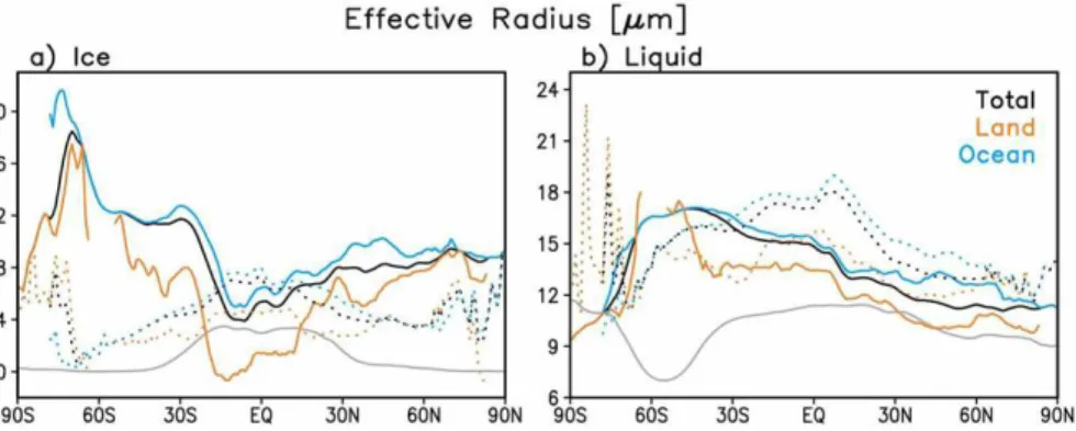
4.3 Cloud particle e_ffective radii

Validation satellite data of cloud particle effective radii are based on radiances emitted by cloud particles in the top part of the cloud seen from above; hence the data

rep-15

resents the near cloud-top cloud particle’s optical properties. The effective radii of ice and liquid cloud particles produced in MAC and CTL simulations are compared against Platnick et al. (2003) satellite data as observations or OBS. Figure 8 shows that the liquid effective radii (r_e_ff_{) of MAC simulation are in the range of 10–18 µm with a global}

average of 14 to 14.4 µm in DJF and JJA seasons. On average,r_e_ff _{is less than the} 20

observed by 1–1.5 µm, which is well within the spread of the observations (not shown). Repeating the same calculation for CTL, the corresponding values of r_e_ff _{are in the}

9–14 µm range with global average values of 10.1 to 10.5 µm for DJF and JJA respec-tively. Thus the CTL effective radii are about 30 % smaller than observed. Indeed MAC is also biased towards the smaller size, but the size in McRAS-AC depends upon the

25

(19)

GMDD

5, 1381–1434, 2012

GEOS-5 AGCM

Y. C. Sud et al.

Title Page

Tables Figures

◭ ◮

Back Close

Full Screen / Esc

Discussion

P

a

per

|

Dis

cussion

P

a

per

|

Discussion

P

a

per

|

Discussio

n

P

a

per

|

The simulated effective radii of cloud ice particles are in 24–42 µm range with an average 28.3 to 29.9 µm for JJA and DJF respectively. Clearly MAC simulates larger effective radii, but again it is about 10 % or 3 µm too large, which is again well within observational uncertainty. In fact 3 µm in 30 µm can be explained easily by the unpre-dictable variations between the e_ffective and volume radius of ice particles. Again in

5

CTL, the empirically estimated ice particle effective radius is ∼3 µm less than the

ob-served, however, its zonal biases tell us that polar ice clouds have problem and that is consistent with their low number and large particle size. The RMSE errors for MAC are twice as large, which is not too surprising because MAC (compared to CTL) has more degrees of freedom which increases uncertainty and variability, hence MAC

sim-10

ulated numbers, being actual predictions, have a large spread whereas CTL values have much less (Fig. 8). Based on these results, MAC simulated liquid and ice cloud-particle effective radii are quite reasonable. Therefore, one infers that on this measure, McRAS-AC performs reasonably well as an aerosol-cloud-radiation interaction model with the current cloud physics. The grid average liquid (ice) particle numbers are about

15

40 (3.8) cm−3_{with corresponding in-cloud values of}

∼90 (10) cm−3. There are very few

global data fields for these, but judging by the radiation imbalances at the top of the atmosphere, one presumes that large biases in MAC simulated numbers again may well be aerosol-input related.

4.4 TOA radiation fields

20

4.4.1 TOA radiation budget

In this subsection we assess briefly the verisimilitude of the radiation budget produced by the 10-yr simulations of GEOS-5 with the two cloud schemes. We compare model simulated TOA LW and SW zonal fluxes to their counterparts from CERES (Loeb et al., 2009, CERES data set EBAF 2.6) in Fig. 9 for DJF, JJA, and ANN fields; corresponding

25

(20)

GMDD

5, 1381–1434, 2012

GEOS-5 AGCM

Y. C. Sud et al.

Title Page

Tables Figures

◭ ◮

Back Close

Full Screen / Esc

Discussion

P

a

per

|

Dis

cussion

P

a

per

|

Discussion

P

a

per

|

Discussio

n

P

a

per

|

observed radiative fields are mostly left for the next subsection which frames the dis-cussion in terms of cloud radiative e_ffects (CRE).

The zonal-average radiation plots, shown in Fig. 9, indicate that for the most part, MAC matches OBS better than CTL. As will be discussed further later, despite MAC’s tropical convective clouds having too little cloud water/ice and somewhat lower height,

5

the resulting outgoing longwave radiation (OLR) and absorbed shortwave radiation (ASW) are closer to observations than CTL whose overactive convection yields too much reflected SW and too little OLR. MAC’s TOA radiation fields diverge, however, more from observations at midlatitudes with too much ASW in the SH summer (dis-cussed extensively below) and too much OLR in the NH summer.

10

MAC and CTL simulations agree with global mean OLR observations to within 2 W m−2 _{(Table 3), but MAC’s RMSE values are better by 1–2 W m}−2 _{for both}

sea-sonal and annual averages, indicating larger spatial error cancellations for CTL. The annual averages of global ASW are about the same for both cloud schemes, and about 2.5 W m−2 _{larger than the observations. However, summer and winter global values} 15

differ substantially between the two schemes. The ASW of MAC differs by∼17 W m−2

between DJF and JJA while the corresponding differences in both observations and CTL are about half. Again, this is a result of biases in the MAC SH midlatitude marine clouds (possible reasons and solutions are discussed later) making the RMSE slightly worse than CTL in DJF (Table 3). The same issue impacts the global net TOA flux

20

which is∼9 W m−2too high for MAC in DJF compared to CERES. The global net TOA

flux for JJA is within∼1 W m−2of observations for both MAC and CTL, but the DJF

er-ror of MAC is too large, yielding a substantial excess of 8.5 W m−2_{in annual global net}

TOA radiation. Our simulations are not much affected by this large energy imbalance because of externally prescribed SSTs. The RMSEs of net TOA radiation are worse for

25

(21)

GMDD

5, 1381–1434, 2012

GEOS-5 AGCM

Y. C. Sud et al.

Title Page

Tables Figures

◭ ◮

Back Close

Full Screen / Esc

Discussion

P

a

per

|

Dis

cussion

P

a

per

|

Discussion

P

a

per

|

Discussio

n

P

a

per

|

are closer to observations than CTL. This is reaffirmed in the next subsection which examines cloud radiative effects.

4.4.2 TOA cloud radiative effect

A well-established way for assessing the influence of clouds on the radiation budget is via the cloud radiative effect (CRE), a quantity also popularly known as cloud

ra-5

diative forcing (Harrison et al., 1990). CRE for either solar/shortwave (SW) or thermal infrared/longwave (LW) radiation is defined as:

CRELW,SW=F_LW,SWcld −F_LW,SWclr (1a)

which can also be recast as

CRELW,SW=Ctot(F_LW,SWovc −F_LW,SWclr ) (1b)

10

under the assumption that the cloudy sky flux can be written as the linear combination of clear and overcast fluxes. In the above,F _{is the net downward (i.e., downward}

mi-nus upward) flux (LW or SW), the superscripts clr designates clear (cloud-free) skies, cld designates all-sky conditions (containing a mixture of cloudy and clear skies), and ovc designates overcast skies (100 % cloud fraction); C_tot _{is the total vertically} pro-15

jected cloud fraction which in the AGCM depends on individual layer cloud fractions and assumptions about their overlap. While both definitions can be used for analyzing observational data, the model CRE always comes from Eq. (1a). Nevertheless, Eq. (1b) is preferable forinterpreting AGCM CRE. For two different cloud schemes producing the sameC_tot_{, the CRE di}_ff_{erences mainly arise from their water path/e}_ff_{ective radius} 20

differences (their combined effect is captured by the cloud optical depth) in the SW, and cloud top height differences in the LW (although optical depth differences also play some role at low values of optical depth) through their effect onFovc_.

The CRE as defined above can be calculated at either TOA or at the surface. Here we only show TOA results for which the observed values are more reliable. In the SW,

(22)

GMDD

5, 1381–1434, 2012

GEOS-5 AGCM

Y. C. Sud et al.

Title Page

Tables Figures

◭ ◮

Back Close

Full Screen / Esc

Discussion

P

a

per

|

Dis

cussion

P

a

per

|

Discussion

P

a

per

|

Discussio

n

P

a

per

|

the CRE TOA is usually negative because the net (absorbed) flux for cloudy skies is smaller than for clear skies. In the LW, the TOA CRE is usually positive because the upward TOA flux is greater under clear skies than cloudy skies (the downward flux is zero in both cases). The CRE of net radiation is, CRE_net=CRE_SW+CRE_LW, and can be positive or negative depending on cloud type. Measurements of TOA CRE are readily

5

available from CERES, among other sources, and can be used for model evaluation. We use the EBAF v. 2.6 of the CERES data set (Loeb et al., 2009).

In an earlier paper, Oreopoulos et al. (2012) showed that for diagnostic radiation cal-culations with a different radiation scheme, the TOA CRE and its sensitivity to cloud vertical distribution of clouds was very different for CTL and MAC clouds. Based on

10

the results of Oreopoulos et al. (2012) we naturally expected substantial CRE di_ff er-ences between MAC and CTL. The TOA CRELW differences between observations and the two model runs are shown in Fig. 10. In this plot as well as similar ones that follow for CRE_SW and CRE_net, red and blue colors represent positive and negative bi-ases with color intensity proportional to the magnitude of the bias. The lighter shade

15

of colors for MAC minus OBS compared to CTL minus OBS is indicative of the overall smaller biases for MAC, and this is especially true over the Pacific. The CRE_LWbiases in both simulations are consistent with those of cloud fraction bias discussed earlier in Sect. 4.2.1. In the ITCZ region, MAC exhibits smaller CRELW than observations, prob-ably because its convective clouds are too low or too thin (or both), while CTL exhibits

20

the opposite behavior, i.e., larger than observed CRELW, suggesting that convective clouds in CTL may be too high and/or too thick and too spatially extensive. In general, the MAC underestimates are lower than the CTL overestimates. Lower cloud tops in MAC may be due to the influence of quadratic entrainment in McRAS-AC versus linear in the standard RAS of the GEOS-5 GCM (Sud and Walker, 2003a). Larger

entrain-25

(23)

GMDD

5, 1381–1434, 2012

GEOS-5 AGCM

Y. C. Sud et al.

Title Page

Tables Figures

◭ ◮

Back Close

Full Screen / Esc

Discussion

P

a

per

|

Dis

cussion

P

a

per

|

Discussion

P

a

per

|

Discussio

n

P

a

per

|

scheme used in CTL (MAC) runs assumes that the convective mass flux increases lin-early (quadratically). By entraining less air compared to McRAS, RAS generates more condensate per unit detrained mass-flux in the convective anvil; naturally, that would require lesser mass flux detrainment to annul the cloud work function (or CAPE) gen-erated in the physics time-step. In other words, both cloud fraction and CRELW would

5

become even more if the entrainment assumption in CTL were made quadratic, with the positive convective CRE_LWbiases would become worse. Another reason for cloud height underestimate by MAC is neglect of convective height increase by freezing of cloud ice and precipitating hydrometeors (Rosenfeld et al., 2006; Koren et al., 2012).

Despite the previously mentioned weaknesses in the simulation of southern

midlati-10

tude ocean clouds by MAC, CRE_LWbiases are not as high because most of the clouds at these latitudes reside in the lower troposphere and do not have much influence on the CRELW. On the other hand, biases in the snow and ice covered polar regions (where, however, observed CREs may be less reliable), both the positive and nega-tive biases are generally larger in MAC than in CTL for reasons that remain currently

15

unidentified. Overall, the CTL scheme underestimates global CRELWby∼4 W m− 2

(Ta-ble 3) despite the systematic overestimates in convective areas. The MAC simula-tion approaches the global observed value within∼1.0–1.5 W m−2and achieves better

RMSE scores than CTL in both the seasonal and annual means by∼1.5–3 W m−2.

Figure 11 shows TOA CRE_SWradiation di_fference maps. CRE_SWfields of CTL minus

20

OBS have deeper colors with more structure compared to those of MAC minus OBS. Large differences in the biases are evident in MAC and CTL over northern midlatitudes in JJA. But the most prominent MAC biases (underestimates) appear in DJF within the 40◦_S–60◦_{S latitude zone where MAC produces too few IPNC (the annual mean}

total water path is reasonable whereas the simulated liquid and ice particle size are

25

(24)

GMDD

5, 1381–1434, 2012

GEOS-5 AGCM

Y. C. Sud et al.

Title Page

Tables Figures

◭ ◮

Back Close

Full Screen / Esc

Discussion

P

a

per

|

Dis

cussion

P

a

per

|

Discussion

P

a

per

|

Discussio

n

P

a

per

|

impact of the latter possibility, we conducted one year run where we reduced the sea-salt aerosol diameter by 50 % across the board resulting in an 8-fold increase in aerosol particle number density (APND). This is a reasonable sensitivity test because GOCART simulates mass balances employing only the mass tendency as sum of sources, sinks, aerosol chemistry and advection; APND for di_fferent bins is estimated from volume

5

radius and density that match the aerosol optical thickness. The 8-fold increase in the sea salt APND resulted in a TOA CRESW field very similar to that of CTL (Fig. 12). While this experiment isolated a likely cause of the bias, it cannot be considered the sole source of the CPNC underestimates. Greater ice particle numbers can also be created by a physically based ice-cloud particle multiplication algorithm. The region

10

is predominantly in the rising branch of the Ferrell cell where winds are strong and gusty, consequently CPNC increases due to cloud particle colliding and shattering, ignored in the current version of McRAS-AC, can be significant. Another mechanism that would increase IPNC is liquid cloud particles glaciating sooner as opposed to being depleted by Bergeron-Findeisen mass exchange between water drops and ice particles

15

through evaporation-deposition process. Eliminating the biases with better algorithms, would not only mitigate the CPNC biases over 40◦_S–60◦_{S, but would have the potential}

benefit of eliminating CRESW biases elsewhere as well. We are actively working on a physically-based solution to this problem.

The similarity of some biases appearing in both simulations suggest either the

in-20

fluence of their common RAS (Moorthi and Suarez, 1992) heritance or other shared model deficiencies such as absence of boundary-layer stratus clouds, and excessive orographic precipitation. Wherever the diagnostics show significantly similar biases in MAC minus OBS and CTL minus OBS, a common cause, not related to aerosol-cloud interaction, is possibly the culprit. Regarding the positive biases (underestimates of

25

(25)

GMDD

5, 1381–1434, 2012

GEOS-5 AGCM

Y. C. Sud et al.

Title Page

Tables Figures

◭ ◮

Back Close

Full Screen / Esc

Discussion

P

a

per

|

Dis

cussion

P

a

per

|

Discussion

P

a

per

|

Discussio

n

P

a

per

|

stratus clouds offwest coast of north and South America as shown in Kay et al. (2012). The current baseline GEOS-5 GCM lacks PBL stratus, and in this exercise, both MAC and CTL simulations exhibit similar CRESW biases due to this inherent flaw(s) in the model’s PBL convection.

The positive CRESW biases in southern midlatitude oceans beneath the Ferrell cell

5

between 40◦_S–60◦_{S are big enough to cause a global mean underestimate of 5 W m}−2

in DJF when the SH insolation peaks. For the same reason, for SH summer, MAC’s RMSE is slightly larger than CTL even though for JJA and ANN the RMSE is notably smaller for MAC. The global ANN CRESW of MAC is 1 W m−

2

too low since the SH summer underestimate is larger than the NH summer overestimate. CTL simulates

10

better the summer SH, but contains in general more bias compensations as evidenced by the larger RMSEs in JJA and ANN.

The bias fields of CRE_net(Fig. 13) reflect previously discussed issues: In areas where CRELW is small, the CRESW biases take over, see for example the SH midlatitude oceans (MAC) and PBL stratus areas (both simulations). MAC fares better in the

in-15

tensely convective regions: apparently it’s CRE_SW and CRE_LW underestimates largely cancel out because they have opposite signs. On the other hand for the CTL the trop-ical overestimates of CRESW are significantly larger than the overestimates of CRELW resulting in too strong (too negative) CRE_net, thus implying that the region loses ra-diative energy at a rate larger than that of CERES observations. Based on the global

20

values of CREnetalone (Table 3), one could erroneously conclude that CTL simulates better cloud fields than MAC. But much of the agreement with CERES is fortuitous and results from cancellations between the SW and LW CREs as well as spatial cancella-tions. Indeed, the MAC RMSEs of CREnetare lower on both the seasonal and annual basis.

25

4.5 Comments on the statistics of circulation

(26)

GMDD

5, 1381–1434, 2012

GEOS-5 AGCM

Y. C. Sud et al.

Title Page

Tables Figures

◭ ◮

Back Close

Full Screen / Esc

Discussion

P

a

per

|

Dis

cussion

P

a

per

|

Discussion

P

a

per

|

Discussio

n

P

a

per

|

for model’s biases but each dataset has its own uncertainties. One naturally likes to find out, where McRAS-AC really made a difference vis- `a-vis the baseline AGCM and whether it is statistically significant and/or beneficial for the climate forecast. Signif-icant changes in precipitation in convective regions are the only easily interpretable differences between MAC and CTL and those were discussed in Sect. 4.1.2. We found

5

some differences in the circulation as well, but most of them were local, i.e., without much large-scale structure. Other significant differences were in limited to the regions, where the input data are sparse, while the 4DDA analysis verification data reflects the influence of the physics of the baseline model; in such regions, the biases are less for CTL simulation as compared to MAC. Its prime example is 100 to 200 hPa

tempera-10

ture biases in the tropics for which 4DDA analysis is a proxy for observations. There is virtually very little data in this region and the 4DDA fields are largely constrained by the background model performing the data assimilation. For GMAO analysis that background model is GEOS-5 GCM with the baseline cloud physics. We decided to postpone this analysis for Part 2 of this paper or until some large biases of McRAS-AC

15

are eliminated through further model development. These analyses are rudimentary, and are included for completeness.

5 Summary and conclusion

We examined 10 yr long simulations with the GEOS-5 GCM with SSTs prescribed from Reynolds et al. (2002) analysis. One simulation uses the baseline model and one uses

20

the McRAS-AC cloud physics in the GEOS-5 GCM, which consists of McRAS cloud physics developed by Sud and Walker (1999a) with several follow-on upgrades (Sud and Walker, 2003a, b), aerosol cloud interaction (using Fountoukis and Nenes (2005) for CCN activation and Barahona and Nenes (2009a, b) for ice nucleation) plus Sud and Lee (2007) two moment calculation for liquid precipitation. In this version of McRAS-AC,

25

(27)

GMDD

5, 1381–1434, 2012

GEOS-5 AGCM

Y. C. Sud et al.

Title Page

Tables Figures

◭ ◮

Back Close

Full Screen / Esc

Discussion

P

a

per

|

Dis

cussion

P

a

per

|

Discussion

P

a

per

|

Discussio

n

P

a

per

|

1. McRAS-AC (MAC) simulation produced comparable circulation and precipitation fields as the baseline GEOS-5 AGCM (CTL) simulation. There are patchy areas with significant differences in the circulation and precipitation fields, but most of the major circulation features are similar. Accordingly, it is difficult to say unequiv-ocally which is better. In the global mean and RMSE biases of precipitation, MAC

5

simulation has a clear edge over the CTL. Nevertheless, large 40◦_S–60◦_{S biases}

in radiative CREs and cloud water path over the storm track regions and even largely missing the low level stratus (both schemes are similarly deficient) does not justify declaring MAC to be better than CTL before additional upgrades. How-ever, we have identified some good strategies that are supported by the

subse-10

quent sensitivity tests included in the paper. Specifically insu_fficient cloud particle numbers over the 40◦_S–60◦_{S regions are categorically related to low sea-salt}

aerosol-particle numbers as well as lack of cloud particle enhancement by colli-sion and splintering. Ice nucleation also lacks full range of IN making aerosols. These are important issues making ice nucleating processes and aerosols to

15

be an active area of research (e.g., DeMott et al., 2011; Sesartic et al., 2011). Similar problems have been pointed out in other models and the general con-sensus is that merely tuning the current algorithms does not solve the problem. The high cloud water path in the storm track region seems to be related to ineffi -cient/insu_fficient wet-scavenging of aerosols in the storms.

20

2. MAC simulates better surface and TOA short and longwave radiative fields and their CREs, but again its potential benefits were largely mitigated by large biases in the aforementioned regions and prescribed SSTs. There are several options for eliminating these biases, but it needs to be determined which of them are most defensible physically. Elsewhere MAC produced better cloud fractions, cloud

25

water and ice paths.