HESSD
11, 6035–6063, 2014Adverse effects of autoregressive
updating of streamflow predictions
M. Li et al.
Title Page
Abstract Introduction
Conclusions References
Tables Figures
◭ ◮
◭ ◮
Back Close
Full Screen / Esc
Printer-friendly Version
Interactive Discussion
Discussion
P
a
per
|
Discus
sion
P
a
per
|
Discussion
P
a
per
|
Discussion
P
a
per
|
Hydrol. Earth Syst. Sci. Discuss., 11, 6035–6063, 2014 www.hydrol-earth-syst-sci-discuss.net/11/6035/2014/ doi:10.5194/hessd-11-6035-2014
© Author(s) 2014. CC Attribution 3.0 License.
This discussion paper is/has been under review for the journal Hydrology and Earth System Sciences (HESS). Please refer to the corresponding final paper in HESS if available.
A strategy to overcome adverse e
ff
ects of
autoregressive updating of streamflow
predictions
M. Li1, Q. J. Wang2, J. C. Bennett2, and D. E. Robertson2
1
CSIRO Computational Informatics, Floreat, Western Australia, Australia
2
CSIRO Land and Water, Highett, Victoria, Australia
Received: 30 April 2014 – Accepted: 21 May 2014 – Published: 10 June 2014 Correspondence to: M. Li ([email protected])
HESSD
11, 6035–6063, 2014Adverse effects of autoregressive
updating of streamflow predictions
M. Li et al.
Title Page
Abstract Introduction
Conclusions References
Tables Figures
◭ ◮
◭ ◮
Back Close
Full Screen / Esc
Printer-friendly Version
Interactive Discussion
Discussion
P
a
per
|
Discus
sion
P
a
per
|
Discussion
P
a
per
|
Discussion
P
a
per
|
Abstract
For streamflow forecasting applications, rainfall–runoff hydrological models are often augmented with updating procedures that correct streamflow predictions based on the latest available observations of streamflow and their departures from model simula-tions. The most popular approach uses autoregressive (AR) models that exploit the
5
“memory” in hydrological model simulation errors. AR models may be applied to raw errors directly or to normalised errors. In this study, we demonstrate that AR models applied in either way can sometimes cause over-correction of predictions. In using an AR model applied to raw errors, the over-correction usually occurs when streamflow is rapidly receding. In applying an AR model to normalised errors, the over-correction
10
usually occurs when streamflow is rapidly rising. Furthermore, when parameters of a hydrological model and an AR model are estimated jointly, the AR model applied to normalised errors sometimes degrades the stand-alone performance of the base hydrological model. This is not desirable for forecasting applications, as predictions should rely as much as possible on the base hydrological model, and updating should
15
be applied only to correct minor errors. To overcome the adverse effects of the ordinary AR models, a restricted AR model applied to normalised errors is introduced. The new model is evaluated on a number of catchments and is shown to reduce over-correction and to improve the performance of the base hydrological model considerably.
1 Introduction 20
Rainfall–runoffmodels are widely used to generate streamflow forecasts, which pro-vide essential information for flood warning and water resources management. For streamflow forecasting, rainfall–runoffmodels are often augmented by updating proce-dures that correct streamflow predictions based on the latest available observations of streamflow and their departures from model predictions. Model prediction errors reflect
HESSD
11, 6035–6063, 2014Adverse effects of autoregressive
updating of streamflow predictions
M. Li et al.
Title Page
Abstract Introduction
Conclusions References
Tables Figures
◭ ◮
◭ ◮
Back Close
Full Screen / Esc
Printer-friendly Version
Interactive Discussion
Discussion
P
a
per
|
Discus
sion
P
a
per
|
Discussion
P
a
per
|
Discussion
P
a
per
|
limitations of the hydrological models in reproducing physical processes as well as inaccuracies in data used to force and evaluate the models.
The most popular updating approach uses autoregressive (AR) models, which ex-ploit the “memory” – more precisely the autocorrelation structure – of prediction errors (Kavetski et al., 2003). Essentially, AR updating uses a linear function of the known
5
prediction errors at previous time steps to anticipate prediction errors in a forecast period. Predictions are then updated according to these anticipated errors. AR updat-ing is conceptually simple and yet generally leads to significantly improved predictions (World Meteorological Organization, 1992). AR updating has been shown to provide equivalent performance to more sophisticated non-linear and nonparametric updating
10
procedures (Xiong and O’Connor, 2002).
In rainfall–runoff modelling, model errors are generally heteroscedastic (i.e., they have heterogeneous variance over time) (Xu, 2001; Kavetski et al., 2003) and non-Gaussian (Bates and Campbell, 2001; Schaefli et al., 2007; Shrestha and Solomatine, 2008). In many applications (Seo et al., 2006; Bates and Campbell, 2001; Salamon and
15
Feyen, 2010; Morawietz et al., 2011), AR models are applied to normalised errors that are considered homoscedastic and Gaussian. Normalisation is often achieved through variable transformation by using, for example, the Box–Cox transformation (Thyer et al., 2002; Bates and Campbell, 2001; Engeland et al., 2010) or, more recently, the log– sinh transformation (Wang et al., 2012; Del Giudice et al., 2013). In other applications
20
(Schoups and Vrugt, 2010; Schaefli et al., 2007), AR models are applied directly to raw errors, but residual errors of the AR models may be explicitly specified as het-eroscedastic and non-Gaussian.
There is no agreement on whether it is better to apply an AR model to normalised or raw errors. Recent work by Evin et al. (2013) found that an AR model applied
25
HESSD
11, 6035–6063, 2014Adverse effects of autoregressive
updating of streamflow predictions
M. Li et al.
Title Page
Abstract Introduction
Conclusions References
Tables Figures
◭ ◮
◭ ◮
Back Close
Full Screen / Esc
Printer-friendly Version
Interactive Discussion
Discussion
P
a
per
|
Discus
sion
P
a
per
|
Discussion
P
a
per
|
Discussion
P
a
per
|
(but does not consider the non-Gaussian distribution of errors). Conversely, Schaefli et al. (2007) pointed out that when an AR model is jointly estimated with a hydrological model, there is a clear advantage in applying an AR model to raw errors rather than normalised (or standardised) errors. Schaefli et al. (2007) found that using raw errors leads to more reliable parameter inference and uncertainty estimation, because the
5
mean error of the predictions is close to zero and therefore the predictions are free of systematic bias. The same is not necessarily true when applying an AR model to normalised errors.
In this study, we evaluate AR models applied to both raw and normalised errors in four catchments. We show that when estimated jointly with a hydrological model, the
10
AR model applied to normalised errors sometimes degrades the stand-alone perfor-mance of the base hydrological model. We also identify that both of these ordinary AR models can sometimes cause over-correction of predictions. We introduce a restricted AR model applied to normalised errors and demonstrate its effectiveness in overcom-ing the adverse effects of the ordinary AR models.
15
2 Autoregressive error models
2.1 Formulations
We denote the observed streamflow and modelled streamflow at time t by Qt and QS,t, respectively. A hydrological model is a function of forcing variables (precipitation and potential evapotranspiration), initial catchment state,S0, and a set of hydrological
20
model parameters,θH. An error model is used to describe the difference betweenQS,t andQt. In this study, we firstly examine two first-order AR error models:
i. an AR error model applied to normalised errors (referred to asAR-Norm) defined by:
Z(N)(Qt)=Z(N)(QS,t)+ρ(N)
n
Z(N)(Qt−1)−Z(N)(QS,t−1) o
+ε(N)t , (1)
HESSD
11, 6035–6063, 2014Adverse effects of autoregressive
updating of streamflow predictions
M. Li et al.
Title Page
Abstract Introduction
Conclusions References
Tables Figures
◭ ◮
◭ ◮
Back Close
Full Screen / Esc
Printer-friendly Version
Interactive Discussion
Discussion
P
a
per
|
Discus
sion
P
a
per
|
Discussion
P
a
per
|
Discussion
P
a
per
|
ii. an AR error model applied to raw errors (referred to asAR-Raw) defined by
Z(R)(Qt)=Z(R)
n
QS,t+ρ(R)(Qt−1−QS,t−1) o
+ε(R)t , (2)
where
Z(Q)=b−1log{sinh(a+bQ)} (3)
is the logarithmic, hyperbolic-sine (log–sinh) transformation (Wang et al., 2012),ρ
5
is the lag-1 autoregression parameter andεt is an identically and independently distributed Gaussian deviate with mean zero and standard deviationσ. We also assumea >0 and b >0. We use superscript(N)and (R)to denote parameters of AR-Norm and AR-Raw models, respectively.
The formulations given by Eqs. (1) and (2) look similar, however the updating
pro-10
cedures differ significantly. Both models represent the lag-one autocorrelation by an AR model structure and both employ the log–sinh transformation. However, the way the log–sinh transformation is applied differs between the two models. The AR-Norm model first applies the log–sinh transformation to the observed and modelled stream-flow, and then applies the autoregression parameterρto the errors of the transformed
15
streamflows. In contrast, the AR-Raw model applies the autoregression parameterρ to the raw errors to update the model prediction, and then applies the log–sinh trans-formation to the observed streamflow and updated model prediction.
The median of the updated streamflow prediction (referred to as updated stream-flow),QU,t, for the AR-Norm and AR-Raw models can be derived respectively by
20
Q(N)U,t=(Z(N))−1hZ(N)(QS,t)+ρ(N)nZ(N)(Qt−1)−Z(N)(QS,t−1)oi, (4) Q(R)U,t=QS,t+ρ(R)(Qt−1−QS,t−1), (5) whereZ−1is the inverse of log–sinh transformation (or back-transformation). The mag-nitude of the error update by the AR-Raw model,Q(R)U,t−QS,t, is dependent only on the
HESSD
11, 6035–6063, 2014Adverse effects of autoregressive
updating of streamflow predictions
M. Li et al.
Title Page
Abstract Introduction
Conclusions References
Tables Figures
◭ ◮
◭ ◮
Back Close
Full Screen / Esc
Printer-friendly Version
Interactive Discussion
Discussion
P
a
per
|
Discus
sion
P
a
per
|
Discussion
P
a
per
|
Discussion
P
a
per
|
difference betweenQt−1and QS,t−1. In contrast, the magnitude of the error update by the AR-Norm model,Q(N)U,t−QS,t, is dependent not only on the difference betweenQt−1 andQS,t−1, but also onQS,t. Put differently, the AR-Norm model uses errors calculated in the transformed domain, and this means that the error in the original domain can be amplified (or reduced) by the back-transformation (Eq. 4). The AR-raw model uses
5
errors calculated in the original domain and no back-transformation is used in Q(R)U,t (Eq. 5), meaning that the error in the original domain cannot be amplified (or reduced). In Appendix A, we show that the AR-Norm model gives greater error updates for larger values ofQS,t.
2.2 Estimation
10
The maximum likelihood estimation is used to estimate the hydrological model param-eters and the error model paramparam-eters jointly. The likelihood functions for the AR-Norm and AR-Raw models can be written respectively as
Lθ(N),θH=Y
t
P(Qt|QS,t,QS,t−1;θ(N),θH)
=Y
t
Jz→Qφ
Z(N)(Qt)−Z(N)(QS,t)−ρ(N)nZ(N)(Qt−1)−Z(N)(QS,t−1)o σ(N)
(6)
Lθ(R),θH=Y
t
P(Qt|QS,t,QS,t−1;θ(R),θH)
=Y
t
Jz→Qφ
Z(R)(Qt)−Z
(R)n
QS,t+ρ(R)(Qt−1−QS,t−1) o
σ(R)
(7)
HESSD
11, 6035–6063, 2014Adverse effects of autoregressive
updating of streamflow predictions
M. Li et al.
Title Page
Abstract Introduction
Conclusions References
Tables Figures
◭ ◮
◭ ◮
Back Close
Full Screen / Esc
Printer-friendly Version
Interactive Discussion
Discussion
P
a
per
|
Discus
sion
P
a
per
|
Discussion
P
a
per
|
Discussion
P
a
per
|
whereJz→Q={tanh(a+bQt)}−1 is the Jacobian determinant of the log–sinh transfor-mation andφ(x) is the standard Gaussian probability density function. The probabil-ity densprobabil-ity function is replaced by the cumulative probabilprobabil-ity function when evaluating events of zero flow occurrences (Wang and Robertson, 2011; Li et al., 2013).
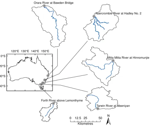
3 Description of case study 5
We test four catchments in southeast Australia, spanning temperate to subtropical cli-mates (Fig. 1, Table 1). The Abercrombie River intermittently experiences periods of very low (to zero) flow, while the other four rivers flow perennially (Table 1). Stream-flow data are taken from the Catchment Water Yield Estimation Tool (CWYET) dataset (Vaze et al., 2011). All catchments have high-quality streamflow records with very few
10
missing data. Rainfall and potential evaporation data are derived from the Australian Water Availability Project (AWAP) dataset (Jones et al., 2009).
We predict daily streamflow with the GR4J rainfall–runoffmodel (Perrin et al., 2003). We apply updating procedures to correct model predictions. We use data from 1992 to 2005 (14 years) and generate 14-fold cross-validated streamflow predictions. The
15
data from 1990–1991 are only used to warm up the GR4J model. For a given year, we leave out the data from that year and the following year when estimating the parame-ters of GR4J and error models. For example, if we wish to predict flows for 1999, we leave out data from 1999 and 2000. The removal of data from the following year (2000) is designed to minimise the impact of hydrological memory on model parameter
esti-20
mation. We then predict streamflows in that year (1999) from the remaining data. All results presented in this paper are based on this cross-validation instead of calibration in order to ensure the results can be generalised to independent data.
To demonstrate the problems of over-correction of errors in updating and poor stand-alone performance of the base hydrological model, we consider only streamflow
pre-25
HESSD
11, 6035–6063, 2014Adverse effects of autoregressive
updating of streamflow predictions
M. Li et al.
Title Page
Abstract Introduction
Conclusions References
Tables Figures
◭ ◮
◭ ◮
Back Close
Full Screen / Esc
Printer-friendly Version
Interactive Discussion
Discussion
P
a
per
|
Discus
sion
P
a
per
|
Discussion
P
a
per
|
Discussion
P
a
per
|
input. In streamflow forecasting, forecasts may be generated from rainfall information that comes from a different source (e.g., a numerical weather prediction model). Our study is aimed at streamflow forecasting applications, so we preserve the distinction between observed and forecast forcings by referring to streamflows modelled with ob-served rainfall assimulationsand those modelled with forecast rainfall aspredictions.
5
As the forecast rainfall we use is observed rainfall, the termspredictions and simula-tionsare interchangeable.
4 Two adverse effects of ordinary AR error models
4.1 Over-correction
The first adverse effect of the ordinary AR models is over-correction of errors in
10
updating. By over-correction, we mean that the AR model updates the hydrological model predictions too greatly. Over-correction is difficult to define precisely, however we will demonstrate the concept with two examples: the first example illustrates over-correction by the AR-Norm model, the second example illustrates over-over-correction by the AR-Raw model.
15
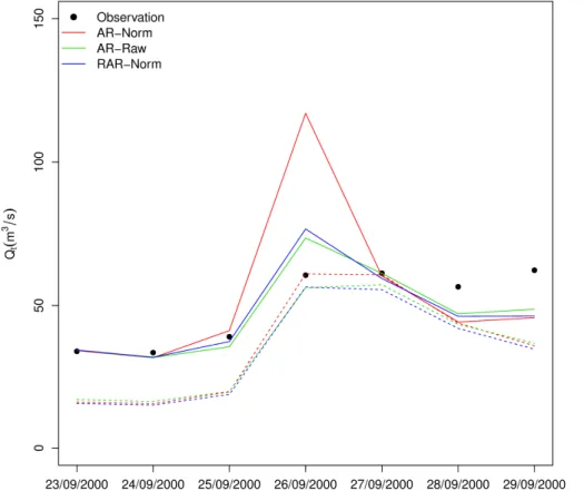
To illustrate the problem of over-correction caused by the AR-Norm model, Fig. 2 presents a 1 week time series for the Mitta Mitta catchment, showing flow predictions with GR4J before error updating (referred to as flows predicted with thebase hydro-logical model) and after error updating (Note that the RAR-Norm model included in Fig. 2 will be introduced and discussed in Sect. 4. The same applies to Figs. 3–7.).
20
Figure 2 shows that the base hydrological models consistently under-estimate the flow from 23 September 2000 to 25 September 2000, and the corresponding updating pro-cedures successfully identify the need to compensate for this under-estimation. For the AR-Norm model, however, the correction amount for 26 September 2000 is unrea-sonably large. Because the predicted flow on 26 September 2000 is much higher than
25
HESSD
11, 6035–6063, 2014Adverse effects of autoregressive
updating of streamflow predictions
M. Li et al.
Title Page
Abstract Introduction
Conclusions References
Tables Figures
◭ ◮
◭ ◮
Back Close
Full Screen / Esc
Printer-friendly Version
Interactive Discussion
Discussion
P
a
per
|
Discus
sion
P
a
per
|
Discussion
P
a
per
|
Discussion
P
a
per
|
the previous day is greatly amplified by the back-transformation, leading to the over-correction. In contrast, the AR-Raw model works better in this situation because the magnitude of the error update never exceeds the prediction error on the previous day regardless of whether the predicted flow is high or low.
Figure 3 shows that about 15–25 % AR-Norm updated predictions have an error
5
update that is larger than the prediction error on the previous day and therefore are susceptible to over-correction. Figure 4 presents a time-series plot for the Orara catch-ment and shows the instances susceptible to over-correction of the AR-Norm model by the vertical inward facing tick-marks. These instances all occur when the flow rises.
A converse example is presented in Fig. 5 where the AR-Raw model causes
over-10
correction. Here, the base hydrological model significantly under-estimates the peak on 6 July 1998. The magnitude of the error update given by the AR-Raw model cannot adjust according to the value of the prediction. As a result, the AR-Raw model updates the prediction on 7 July 1998 with a very large amount, resulting in over-estimation. In contrast, the AR-Norm model does a better job in this example, giving a smaller
15
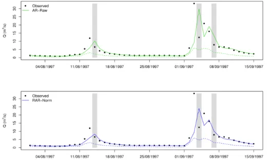
magnitude of error update by recognising that the hydrograph is moving downward. It is generally true that in applying the AR-Raw model, over-correction may occur when the flow is receding. Figure 6 provides more examples of the over-correction caused by the AR-Raw model from a longer time-series plot for the Abercrombie catchment. There are three clear instances of over-correction, all occurring on the time step immediately
20
after large peaks in observed flows.
4.2 Poor stand-alone performance of the base hydrological model
The second issue with conventional AR error models is the stand-alone performance of the base hydrological model (GR4J). As noted above, the parameters of the base hy-drological model are those estimated jointly with an AR model. For streamflow
forecast-25
medium-HESSD
11, 6035–6063, 2014Adverse effects of autoregressive
updating of streamflow predictions
M. Li et al.
Title Page
Abstract Introduction
Conclusions References
Tables Figures
◭ ◮
◭ ◮
Back Close
Full Screen / Esc
Printer-friendly Version
Interactive Discussion
Discussion
P
a
per
|
Discus
sion
P
a
per
|
Discussion
P
a
per
|
Discussion
P
a
per
|
range rainfall forecasts) error updating becomes less effective, and the performance of the base hydrological model is crucial for realistic forecasts. While we investigate only forecasts at a lead time of one timestep in this study, we aim to develop methods that can be applied to forecasts at longer lead times. Further, if the base hydrological model does not replicate important catchment processes realistically, the performance of the
5
hydrological model outside the calibration period may be less robust.
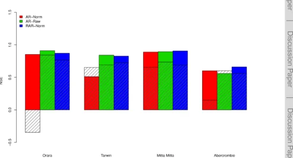
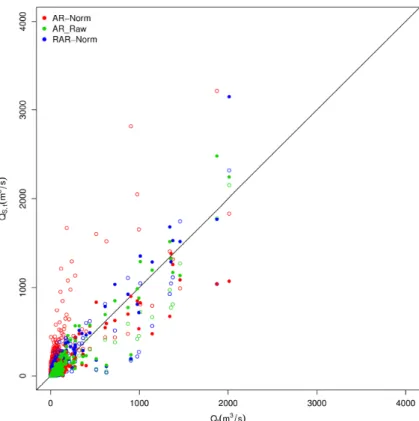
Figure 7 presents the Nash–Sutcliffe efficiency (NSE) (Nash and Sutcliffe, 1970) cal-culated from the base hydrological model and the error models. When the AR-Norm model is used, the predicted flows from the base hydrological model are very poor for the Orara catchment (NSE<0). The scatter plot in Fig. 8 shows further detail about
10
the streamflow prediction for the Orara catchment. When the AR-Norm model is used, the base hydrological model greatly over-estimates discharge and the AR-Norm model then attempts to correct this systematic over-estimation. This is also shown in Fig. 4 where the base hydrological model has a strong tendency to over-estimate flows for a range of flow magnitudes. The base hydrological model with the AR-Norm model
15
also performs poorly for the Abercrombie catchment (Fig. 7). In this case, the base hy-drological model tends to under-estimate flows (results not shown). For the other three catchments, however, the base hydrological model with the AR-Norm model performs reasonably well.
In general, the AR-Raw base hydrological model performs as well or better than
20
the AR-Norm base hydrological model. The AR-Raw base hydrological model is no-tably better than the AR-Norm base hydrological model in the Abercrombie and Orara catchments (Fig. 7). This suggests that more robust performance can be expected of base hydrological models when AR models are applied to raw errors.
We note that for both the AR-Raw model and the AR-Norm models, the updated
25
HESSD
11, 6035–6063, 2014Adverse effects of autoregressive
updating of streamflow predictions
M. Li et al.
Title Page
Abstract Introduction
Conclusions References
Tables Figures
◭ ◮
◭ ◮
Back Close
Full Screen / Esc
Printer-friendly Version
Interactive Discussion
Discussion
P
a
per
|
Discus
sion
P
a
per
|
Discussion
P
a
per
|
Discussion
P
a
per
|
AR-Norm base hydrological model in the Tarwin catchment. This points to a tendency to overfit the parameters to the calibration period, resulting in the error model undermining the performance of the base hydrological model under cross-validation. Such a lack of robustness is highly undesirable in forecasting applications, where the hydrological models should be able to operate in conditions that differ from those experienced during
5
calibration.
5 Restricted AR error model
Motivated to overcome the potential for over-correction, we modify the AR-Norm model by restricting the magnitude of its corrections. This is a restricted AR–Norm model, which we call the RAR-Norm model. The RAR-Norm model is defined by
10
Z(R)(Qt)=
Z(R)(QS,t)+ε(R)t + ρ(R)nZ(R)(Qt−1)−Z
(R)
(QS,t−1)
o if|QM,t−QS,t| ≤ |Qt−1−QS,t−1| Z(R)(QS,t+Qt−1−QS,t−1)+ε
(R)
t otherwise
(8)
where the superscript(R)is used to denote the parameters of the RAR-Norm model and QM,t=(Z(R))−1hZ(R)(QS,t)+ρ(R)nZ(R)(Qt−1)−Z(R)(QS,t−1)oi is the updated stream-flow prediction median given by the AR-Norm model without restriction. The actual
15
updated streamflow prediction median of the RAR-Norm model is given by
Q(R)U,t= (
QM,t if|QM,t−QS,t|<|Qt−1−QS,t−1|
QS,t+Qt−1−QS,t−1 otherwise (9)
The RAR-Norm model parameters may be jointly estimated with the hydrological model parameters using the maximum likelihood method, in the same as for the AR-Norm and
20
HESSD
11, 6035–6063, 2014Adverse effects of autoregressive
updating of streamflow predictions
M. Li et al.
Title Page
Abstract Introduction
Conclusions References
Tables Figures
◭ ◮
◭ ◮
Back Close
Full Screen / Esc
Printer-friendly Version
Interactive Discussion
Discussion
P
a
per
|
Discus
sion
P
a
per
|
Discussion
P
a
per
|
Discussion
P
a
per
|
The idea behind the RAR-Norm model is simple. We use the AR-Norm model for error updating if the magnitude of the error update is not too large. Otherwise, we adopt a naïve updating scheme, which applies the raw error from the previous time step to correct the current prediction. At any timet, the magnitude of the error update is restricted to a maximum of|Qt−1−QS,t−1|.
5
Because the RAR-Norm model imposes an upper limit on the size of the correc-tion, it effectively reduces the tendency for over-correction. Figure 2 shows that the RAR-Norm model behaves similarly to the AR-Raw model for correcting the peak on 26 September 2000 and avoids the over-correction made by the AR-Norm model. The RAR-Norm model is also able to adjust the magnitude of the error update
accord-10
ing to QS,t and this is particularly useful when the hydrograph is moving downward. Figure 5 shows that when the hydrograph recedes rapidly, the RAR-Norm model pro-duces updated streamflow similar to the AR-Norm model. In this case, the RAR-Norm model avoids the over-correction by the AR-Raw model on 7 July 1998. Similarly, the RAR-Norm works better than the AR-Raw model to avoid the three instances of
over-15
correction for the Abercrombie catchment (Fig. 6). Overall, the RAR-Norm model takes a conservative position when flow changes rapidly, either rising or falling. When flow changes rapidly, it is difficult to anticipate the magnitude of prediction error. Accordingly the AR models are prone to over-correction in such instances.
Figure 3 provides the proportion of the instances where|QM,t−QS,t|>|Qt−1−QS,t−1|.
20
These instances are susceptible to over-correction by the AR-Norm model. The fre-quency of these instances varies somewhat from catchment to catchment. The RAR-Norm model identifies 15–30 % of the time series as possible instances of problematic updating, and the AR-Norm model identifies a similar number of instances (slightly fewer – they are not identical because the parameters for each model are inferred
in-25
HESSD
11, 6035–6063, 2014Adverse effects of autoregressive
updating of streamflow predictions
M. Li et al.
Title Page
Abstract Introduction
Conclusions References
Tables Figures
◭ ◮
◭ ◮
Back Close
Full Screen / Esc
Printer-friendly Version
Interactive Discussion
Discussion
P
a
per
|
Discus
sion
P
a
per
|
Discussion
P
a
per
|
Discussion
P
a
per
|
the RAR-Norm model is largely applied to the instances where the AR-Norm model is susceptible to over-correction.
The RAR-Norm model generally improves the performance of the base hydrological model, in particular compared to the AR-Norm model (Fig. 7). The RAR-Norm base hydrological model performs similarly to, or better than, the base hydrological models
5
of the AR-Norm and AR-Raw model. The improvement over the AR-Norm base hy-drological model is especially evident for the Orara (Figs. 4 and 7) and Abercrombie catchments (Figs. 7).
In general, the updated predictions from the RAR-Norm model show similar or bet-ter predictive accuracy, as measured by NSE, than both the AR-Raw model and the
10
AR-Norm model (Fig. 7). We note that the Orara catchment is an exception: here the AR-Raw model shows slightly better performance than both the AR-Norm and RAR-Norm models. Conversely, the RAR-RAR-Norm model shows notably better performance than both the AR-Norm and AR-Raw models in the Abercrombie catchment. This sug-gests the RAR-Norm model may work better in intermittently flowing catchments,
al-15
though further testing is required to establish that this is true for a greater range of catchments.
Importantly, the updated predictions of the RAR-Norm model outperform the base hydrological model predictions in all catchments. This shows that for the RAR-Norm model, both the base hydrological model and the error updating perform robustly under
20
cross-validation. This is not true of the AR-Raw model in the Abercrombie catchment or for the AR-Norm model in the Tarwin catchment. As noted above, robust perfor-mance under cross-validation, and consistent interaction between the base hydrolog-ical model and the error updating, are crithydrolog-ically important for forecasting applications, where models should perform well in conditions that may differ substantially from those
25
HESSD
11, 6035–6063, 2014Adverse effects of autoregressive
updating of streamflow predictions
M. Li et al.
Title Page
Abstract Introduction
Conclusions References
Tables Figures
◭ ◮
◭ ◮
Back Close
Full Screen / Esc
Printer-friendly Version
Interactive Discussion
Discussion
P
a
per
|
Discus
sion
P
a
per
|
Discussion
P
a
per
|
Discussion
P
a
per
|
6 Discussion and conclusions
For streamflow forecasting, rainfall–runoffmodels are often augmented with an updat-ing procedure that corrects the prediction usupdat-ing information from recently observed prediction errors. The most popular updating approach uses autoregressive (AR) mod-els that exploit the “memory” in model prediction errors. AR modmod-els may be applied to
5
raw errors directly or to normalised errors.
We demonstrate two adverse effects of AR error updating procedures by case stud-ies of four catchments. The first adverse effect is possible over-correction. The updating procedure may correct hydrological predictions too much at some events. The over-correction often happens at the peak or on the rise of a hydrograph for the AR-Norm
10
model and when the hydrograph is receding for the AR-Raw model.
The second adverse effect is poor stand-alone performance of base hydrological models when the parameters of rainfall–runoffand error models are jointly estimated with the AR parameters. We show that poor base hydrological model performance is particularly prevalent in the AR-Norm model. The poor performance appears to occur
15
in catchments with highly skewed streamflow observations (the Abercrombie, an inter-mittent river, and the Orara, a catchment in a subtropical climate). For example, in the Orara River, the base hydrological model tends to greatly over-estimate streamflows, and then relies on the error updating to correct the over-estimates. This is not desirable in real-time forecasting applications for two major reasons. First, modern streamflow
20
forecasting systems often extend forecast lead-times with rainfall forecast information (e.g. Bennett et al., 2014). Updating becomes less effective at longer lead times, and predictions at longer lead times rely on the performance of the base hydrological model. Second, hydrological models are designed to simulate various components of natural systems, such as baseflow processes or overland flow. In theory, simulating these
pro-25
HESSD
11, 6035–6063, 2014Adverse effects of autoregressive
updating of streamflow predictions
M. Li et al.
Title Page
Abstract Introduction
Conclusions References
Tables Figures
◭ ◮
◭ ◮
Back Close
Full Screen / Esc
Printer-friendly Version
Interactive Discussion
Discussion
P
a
per
|
Discus
sion
P
a
per
|
Discussion
P
a
per
|
Discussion
P
a
per
|
catchment, the hydrological model may be much less robust outside the parameter estimation period.
In addition, our results for the AR-Norm and AR-Raw models indicate that the in-teraction between the error updating and the base hydrological model may not always be robust under cross-validation. In some catchments, the updated predictions of the
5
AR-Norm and AR-Raw models were actually worse than the predictions generated by their respective base hydrological models. In forecasting applications, both the base hydrological model and the error updating should perform robustly outside the calibra-tion period, as forecasts are always generated with forcing data that are independent of the calibration period.
10
The adverse effects of AR-Norm error correction discussed in this study are proba-bly generic. In particular, transformations other than the log–sinh transformation may still lead to over-correction at the peak of hydrograph. The proof in Appendix A shows that if a transformation satisfies some conditions (first derivate is positive and second derivate is negative), it will tend to correct more for higher predicted flow and can cause
15
the problem of over-correction. The conditions given by Appendix A are generally true for many other transformations used for data normalization and variance stabilization in hydrological applications, such as logarithm transformation and Box–Cox transfor-mation with the power parameter less than 1.
We use joint parameter inference to calibrate hydrological model and error model
20
parameters, in order to address the true nature of underlying model errors. Inferring parameters of the error model and the base hydrological model independently – i.e., first inferring parameters of the base hydrological model, holding these constant and then inferring the error model parameters – relies on simplified and often invalid er-ror assumptions (it assumes independent, homoscedastic and Gaussian erer-rors), but
25
HESSD
11, 6035–6063, 2014Adverse effects of autoregressive
updating of streamflow predictions
M. Li et al.
Title Page
Abstract Introduction
Conclusions References
Tables Figures
◭ ◮
◭ ◮
Back Close
Full Screen / Esc
Printer-friendly Version
Interactive Discussion
Discussion
P
a
per
|
Discus
sion
P
a
per
|
Discussion
P
a
per
|
Discussion
P
a
per
|
In order to mitigate the adverse effects of ordinary AR updating procedures, we intro-duce a new updating procedure called the RAR-Norm model. The RAR-Norm model is essentially a modification of the AR-Norm model. This new model is able to adjust the magnitude of the error update according to the value of the hydrological predic-tion, which is similar to the AR-Norm model. However, it limits the magnitude of the
5
error update to the prediction error at the previous time step. We show that the new model indeed guards against over-correction and at the same time leads to more ro-bust performance by the base hydrological models. In addition, the performance of the base hydrological model and the error updating are robust under cross validation. Ac-cordingly, we contend that the RAR-Norm model is preferable to both AR-Norm and
10
AR-Raw models for streamflow forecasting applications.
Appendix A:
We will analytically show that the AR-Norm model gives a larger magnitude of the error update for a higher predicted flow.
Firstly, we will show that the first derivate of the log–sinh transform Z defined by
15
Eq. (3) is positive and the second derivate is negative (i.e.Z′(Q)>0 andZ′′(Q)<0) for anyb >0 and anyQ. Following some simple manipulation, we have
Z′(Q)=cosh(a+bQ)
sinh(a+bQ) >0 andZ ′′(Q)
= −b
sinh2(a+bQ)
<0 (A1)
Using the differentiation of inverse functions, we find the first and second derivates of the inverse transformZ−1
20
[Z−1]′(Q)= 1
Z′{Z−1(Q)} >0 and [Z
−1]′′(Q)
=−Z
′′{Z−1 (Q)}
[Z′{Z−1(Q)}]3 >0, (A2)
HESSD
11, 6035–6063, 2014Adverse effects of autoregressive
updating of streamflow predictions
M. Li et al.
Title Page Abstract Introduction Conclusions References Tables Figures ◭ ◮ ◭ ◮ Back Close
Full Screen / Esc
Printer-friendly Version Interactive Discussion Discussion P a per | Discus sion P a per | Discussion P a per | Discussion P a per |
Next, we will derive the difference of magnitudes of the error update between low and high predicted flows. For the sake of notation simplicity, we rewrite q=Z(QS,t)
and u=ρ(T){Z(Qt−1)−Z(QS,t−1)}and assume that u >0. Using Eq. (4), the updated streamflow can be written asQ(N)U,t=Z−1(q+u). The magnitude of the error update can be written as
5
QS,t−Q (N) U,t =
Z−1(q+u)−Z−1(q) =
(Ru
0[Z −1
]′(x+q)dx ifu >0 R0
u[Z
−1
]′(x+q)dx otherwise. (A3)
Suppose that we have two predicted streamflows Q(1)S,t≤QS,(2)t and denote the nor-malised predicted streamflow by q1=ZQS,(1)
t
and q2=ZQ(2)S,
t
and the updated
streamflow byQ(N,1)U,t andQ(N,2)U,t . BecauseZ is an increasing function, we haveq1≤q2.
10
The difference in the magnitude of the error update between Q(1)S,t and Q(2)S,t can be derived as
Q
(1) S,t−Q
(N,1) U,t − Q (2) S,t−Q
(N,2) U,t = Ru 0 n
[Z−1]′(x+q1)−[Z−1]′(x+q2)odx ifu >0 R0
u
n
[Z−1]′(x+q1)−[Z−1]′(x+q2)odx otherwise.
(A4)
From Eq. (A2), we have shown that [Z−1]′ is a positive increasing function and this
15
ensures that [Z−1]′(x+q1)−[Z−1]′(x+q2)≤0. Finally we have
Q
(1) S,t−Q
(N,1) U,t ≤ Q (2) S,t−Q
(N,2) U,t
. (A5)
HESSD
11, 6035–6063, 2014Adverse effects of autoregressive
updating of streamflow predictions
M. Li et al.
Title Page
Abstract Introduction
Conclusions References
Tables Figures
◭ ◮
◭ ◮
Back Close
Full Screen / Esc
Printer-friendly Version
Interactive Discussion
Discussion
P
a
per
|
Discus
sion
P
a
per
|
Discussion
P
a
per
|
Discussion
P
a
per
|
Acknowledgements. This work is part of the WIRADA (Water Information Research and De-velopment Alliance) streamflow forecasting project funded under CSIRO Water for a Healthy Country Flagship. We would like to thank Durga Shrestha for valuable suggestions that led to substantial strengthening of the manuscript.
References 5
Bates, B. C. and Campbell, E. P.: A Markov chain Monte Carlo scheme for parameter estima-tion and inference in conceptual rainfall–runoffmodeling, Water Resour. Res., 37, 937–947, doi:10.1029/2000wr900363, 2001.
Bennett, J. C., Robertson, D. E., Shrestha, D. L., Wang, Q. J., Enever, D., Hapuarachchi, P., and Tuteja, N. K.: A new system for continuous hydrological ensemble forecasting (SCHEF)
10
to lead times of 9 days, J. Hydrol., submitted, 2013.
Del Giudice, D., Honti, M., Scheidegger, A., Albert, C., Reichert, P., and Rieckermann, J.: Im-proving uncertainty estimation in urban hydrological modeling by statistically describing bias, Hydrol. Earth Syst. Sci., 17, 4209–4225, doi:10.5194/hess-17-4209-2013, 2013.
Engeland, K., Renard, B., Steinsland, I., and Kolberg, S.: Evaluation of
statisti-15
cal models for forecast errors from the HBV model, J. Hydrol., 384, 142–155, doi:10.1016/j.jhydrol.2010.01.018, 2010.
Evin, G., Kavetski, D., Thyer, M., and Kuczera, G.: Pitfalls and improvements in the joint in-ference of heteroscedasticity and autocorrelation in hydrological model calibration, Water Resour. Res., 49, 4518–4524, doi:10.1002/wrcr.20284, 2013.
20
Jones, D. A., Wang, W., and Fawcett, R.: High-quality spatial climate data-sets for Australia, Aust. Meteorol. Oceanogr. J., 58, 233–248, 2009.
Kavetski, D., Franks, S. W., and Kuczera, G.: Confronting input uncertainty in environmen-tal modelling, in: Calibration of Watershed Models, edited by: Duan, Q., Gupta, H. V., Sorooshian, S., Rousseau, A. N., and Turcotte, R., American Geophysical Union,
Wash-25
ington DC, 49–68, 2003.
HESSD
11, 6035–6063, 2014Adverse effects of autoregressive
updating of streamflow predictions
M. Li et al.
Title Page
Abstract Introduction
Conclusions References
Tables Figures
◭ ◮
◭ ◮
Back Close
Full Screen / Esc
Printer-friendly Version
Interactive Discussion
Discussion
P
a
per
|
Discus
sion
P
a
per
|
Discussion
P
a
per
|
Discussion
P
a
per
|
Morawietz, M., Xu, C.-Y., and Gottschalk, L.: Reliability of autoregressive error models as post-processors for probabilistic streamflow forecasts, Adv. Geosci., 29, 109–118, doi:10.5194/adgeo-29-109-2011, 2011.
Nash, J. E. and Sutcliffe, J. V.: River flow forecasting through conceptual models part I – A dis-cussion of principles, J. Hydrol., 10, 282–290, doi:10.1016/0022-1694(70)90255-6, 1970.
5
Perrin, C., Michel, C., and Andreassian, V.: Improvement of a parsimonious model for stream-flow simulation, J. Hydrol., 279, 275–289, doi:10.1016/S0022-1694(03)00225-7, 2003. Salamon, P. and Feyen, L.: Disentangling uncertainties in distributed hydrological modeling
using multiplicative error models and sequential data assimilation, Water Resour. Res., 46, W12501, doi:10.1029/2009wr009022, 2010.
10
Schaefli, B., Talamba, D. B., and Musy, A.: Quantifying hydrological modeling errors through a mixture of normal distributions, J. Hydrol., 332, 303–315, doi:10.1016/j.jhydrol.2006.07.005, 2007.
Schoups, G. and Vrugt, J. A.: A formal likelihood function for parameter and predictive infer-ence of hydrologic models with correlated, heteroscedastic, and non-Gaussian errors, Water
15
Resour. Res., 46, W10531, doi:10.1029/2009wr008933, 2010.
Seo, D.-J., Herr, H. D., and Schaake, J. C.: A statistical post-processor for accounting of hy-drologic uncertainty in short-range ensemble streamflow prediction, Hydrol. Earth Syst. Sci. Discuss., 3, 1987–2035, doi:10.5194/hessd-3-1987-2006, 2006.
Shrestha, D. L. and Solomatine, D. P.: Data-driven approaches for estimating
un-20
certainty in rainfall–runoff modelling, Int. J. River Basin Manage., 6, 109–122, doi:10.1080/15715124.2008.9635341, 2008.
Thyer, M., Kuczera, G., and Wang, Q. J.: Quantifying parameter uncertainty in stochastic models using the Box–Cox transformation, J. Hydrol., 265, 246–257, doi:10.1016/S0022-1694(02)00113-0, 2002.
25
Vaze, J., Perraud, J. M., Teng, J., Chiew, F. H. S., Wang, B., and Yang, Z.: Catchment Water Yield Estimation Tools (CWYET), the 34th World Congress of the International Association for Hydro-Environment Research and Engineering: 33rd Hydrology and Water Resources Symposium and 10th Conference on Hydraulics in Water Engineering, Brisbane, 2011. Wang, Q. J. and Robertson, D. E.: Multisite probabilistic forecasting of seasonal
30
HESSD
11, 6035–6063, 2014Adverse effects of autoregressive
updating of streamflow predictions
M. Li et al.
Title Page
Abstract Introduction
Conclusions References
Tables Figures
◭ ◮
◭ ◮
Back Close
Full Screen / Esc
Printer-friendly Version
Interactive Discussion
Discussion
P
a
per
|
Discus
sion
P
a
per
|
Discussion
P
a
per
|
Discussion
P
a
per
|
Wang, Q. J., Shrestha, D. L., Robertson, D. E., and Pokhrel, P.: A log–sinh transforma-tion for data normalizatransforma-tion and variance stabilizatransforma-tion, Water Resour. Res., 48, W05514, doi:10.1029/2011WR010973, 2012.
World Meteorological Organization: Simulated Real-Time Intercomparison of Hydrological Models, World Meteorological Organization, Geneva, Switzerland, 1992.
5
Xiong, L. H. and O’Connor, K. M.: Comparison of four updating models for real-time river flow forecasting, Hydrolog. Sci. J., 47, 621–639, doi:10.1080/02626660209492964, 2002. Xu, C. Y.: Statistical analysis of parameters and residuals of a conceptual water
bal-ance model – methodology and case study, Water Resour. Manag., 15, 75–92, doi:10.1023/A:1012559608269, 2001.
HESSD
11, 6035–6063, 2014Adverse effects of autoregressive
updating of streamflow predictions
M. Li et al.
Title Page
Abstract Introduction
Conclusions References
Tables Figures
◭ ◮
◭ ◮
Back Close
Full Screen / Esc
Printer-friendly Version
Interactive Discussion
Discussion
P
a
per
|
Discus
sion
P
a
per
|
Discussion
P
a
per
|
Discussion
P
a
per
|
Table 1.Basic catchment characteristics.
Name Gauge Site Area Rainfall Streamflow Runoff Zero (km2) (mm yr−1) (mm yr−1) coefficient flows
HESSD
11, 6035–6063, 2014Adverse effects of autoregressive
updating of streamflow predictions
M. Li et al.
Title Page
Abstract Introduction
Conclusions References
Tables Figures
◭ ◮
◭ ◮
Back Close
Full Screen / Esc
Printer-friendly Version
Interactive Discussion
Discussion
P
a
per
|
Discus
sion
P
a
per
|
Discussion
P
a
per
|
Discussion
P
a
per
|
Orara River at Bawden Bridge
150°E 140°E 130°E 120°E
10°S
20°S
30°S
40°S
0 12.5 25 50
Kilometres
Abercrombie River at Hadley No. 2
Mitta Mitta River at Hinnomunjie
Tarwin River at Meeniyan Forth River above Lemonthyme
HESSD
11, 6035–6063, 2014Adverse effects of autoregressive
updating of streamflow predictions
M. Li et al.
Title Page
Abstract Introduction
Conclusions References
Tables Figures
◭ ◮
◭ ◮
Back Close
Full Screen / Esc
Printer-friendly Version
Interactive Discussion
Discussion
P
a
per
|
Discus
sion
P
a
per
|
Discussion
P
a
per
|
Discussion
P
a
per
|