ISSN 1549-3636
© 2005 Science Publications
Corresponding Author: Marco Di Marzio, DMQTE, G.d'Annunzio University, Italy
Boosted Regression Estimates of Spatial Data: Pointwise Inference
1
Marco Di Marzio and
2Charles C. Taylor
1
DMQTE, G.d'Annunzio University, Italy
2
Department of Statistics, University of Leeds, UK
Abstract: In this study simple nonparametric techniques have been adopted to estimate the trend surface of the Swiss rainfall data. In particular we employed the Nadaraya-Watson smoother and in addition, an adapted-by boosting-version of it. Additionally, we have explored the use of the Nadaraya-Watson estimator for the construction of pointwise confidence intervals. Overall, boosting does seem to improve the estimate as much as previous examples and the results indicate that cross-validation can be successfully used for parameter selection on real datasets. In addition, our estimators compare favorably with most of the techniques previously used on this dataset.
Key words: Boosting, coverage rate, cross validation, machine learning, Nadaraya-Watson estimator. INTRODUCTION
Machine learning (Michie et al.[1] p. 2) is generally taken to encompass automatic computing procedures based on logical or binary operations, that learn a task from a series of examples. Attention has mostly focused on methods developed for discrimination tasks. In this case the data take the form {(xi, yi), i=1,…,n}, where
i i1 ip
x =(x ,…, x )T is an attribute vector and i
y ∈ =G {1,…,g} is a class label. Given such data, the goal is to estimate a rule, say δ : ℝp→G , which will assign a new observation x to a class in G . The rule is assessed by comparing the true class of x (which is not used in the learning ofδ) with the predicted class. Since different methods will produce different rules, the methods themselves are then judged by the quality of the rule that is output, though this is highly dependent on the type and quantity of data which is available. Boosting (Shapire[2]; Freund[3]) has become a popular method in machine learning. Given that the goal is to obtain rules which are as accurate as possible, the basic idea of boosting is to enhance a method by adaptation, whereby the rule is modified according to its performance on the original data. More specifically, a B-steps boosting algorithm iteratively computes B estimates by applying a given method, called a weak learner, to B different re-weighted samples. The estimates are then combined into a single one which is the final output. This ensemble rule can be viewed as a “powerful committee”, which is expected to be significantly more accurate than every single estimate. In the original setting, the weak learner was a classification tree, often with only one split (and hence weak), but recently other classifiers have been boosted. Statistical learning (Vapnik[4]) has been used to encompass three previously used methods within
statistical data analysis: density estimation (often referred to as unsupervised learning and a prelude to cluster analysis) discrimination (sometimes called classification, or pattern recognition) and regression (or prediction). All three are commonly used in real-life applications and each has its own historical development. In all three domains, methods exist which make use of a kernel function (kernel density estimation, kernel classifiers and kernel regression); these are often referred to as simply “nonparametric”. Making use of these kernel methods, Di Marzio and Taylor[5-7] have indicated how boosting derives its success: namely, by reducing the bias of the estimators, with only moderate increases in variance. Using this result, one is able to use larger smoothing parameters and improve the overall quality of the final estimate. Other insights into why boosting works are given by Bülmann and Yu[8] (who consider boosting of splines in regression), Friedman et al.[9] (who use logistic regression in classification) and Friedman[10].
methods of optimal selection of (h, B) and since the data have been previously studied we are also then able to compare our results with alternative methods. Finally, we consider the problem of obtaining confidence intervals for the predictions.
EXPLORATORY DATA ANALYSIS
In 1997 the AI-GEOSTATS mailing list set up a “Spatial Interpolation Comparison”. The participants were asked to estimate the daily rainfall values at 367 locations using data of 100 observed measurements (at different locations on the same day). Only after the predictions were made, was the actual data made available. Further details are given, with the results of the competition, in Dubois et al.[11].
The training data were 100 randomly selected sites from a database of 467 sites in Switzerland. The response variable was the amount of rainfall on 8th May 1986 (measured in 1/10th mm). Fig. 1 shows the locations of the training data and the test data points. It is perhaps slightly unusual that the number of training points should be so much smaller than the number of test points.
A summary of the rainfall data (training values) is y=180.15and sd(y)=116.68.
As a first, very naive prediction of the test data, we simply consider y and this gives a root mean squared error (RMSE) value of 111.14. We also note that a naive 95% confidence interval y± ×2 sd(y)has constant width 466.72 and actually contains 355 / 367=96.73%of the test data.
However, these predictions take no account whatsoever of the spatial structure and correlations within the data. A slightly less naive approach is to use a nearest-neighbour prediction, that is to predict the test value y by the training observation i yj such that
k i k
j=arg min d(x , x ), with d denoting the euclidean distance between the sites xi and xk . This nearest neighbour predictor gives a RMSE of 84.17, but no confidence interval is readily available.
A digital elevation model was also made available and this is also shown as an image in Fig. 1. Rainfall often depends on elevation and so the nature and strength, of this relationship was explored. We note that height above sea level, s, can be negative, whereas rainfall y≥0 in general. There may be physical models available but throughout this study, we adopt the principle of letting the data speak for themselves. In Switzerland all the elevationss≥ >c 0 where c≈200, so we can consider transformations of the form: yαwithα>0and sβorlog(s) and then a linear model.
Fig. 1: Location of the measurement sites (black points indicate the training data and gray points the test data) and the relief map showing the height above sea level of the Swiss region.
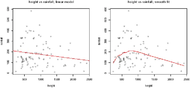
A plot of the data and the smooth fit shown in Fig. 2 suggests a quadratic model may fit tolog(s) .
The residual plots from the first fitted model indicate some shortcomings (Fig. 3), so we also tried a transformation of the response variable and this seemed to improve the fit somewhat. The final fitted model has three estimated parameters and is given by
2
y=13.86 4.06(log(s) 6.65)− −
which gives R-squared=0.095and a RMSE of 112.52, whereas the null model has a RMSE of 116.09. The diagnostic plots are shown in Fig. 3.
Fig. 2: Dependence of rainfall on height. Left: scatter plot with linear fitted line. Right: scatter plot with smooth fit.
NONPARAMETRIC METHODS
Motivation: The most studied and used interpolation technique is kriging (see, for example, Stein[12]). Unfortunately, standard kriging yields unbiased predictions only if restrictive assumptions - typically some kind of stationarity or isotropy - are satisfied. Thereby, a rigorous check of them is always necessary. In fact, a model might not hold across all spatial observations, especially if large spatial datasets are used.
In the last three decades, a number of recent researchers focus on nonparametric regression techniques as a flexible alternative to kriging. A nonparametric analysis seems suitable for exploratory purposes in the selection stage of a parametric model, or if the information on the specific case study does not allow parametric assumptions at all. We can distinguish two tendencies: entirely nonparametric or mixed approaches, in which nonparametric techniques and kriging coexist. A brief outline follows.
In pioneering research, Yakowitz and Sziradowsky[13] study the robustness of kriging in the cases of perturbed data and incorrect variogram selection. As a more robust alternative to kriging, they extensively discuss a fully nonparametric regression technique. In their examples, the nonparametric estimator performs similarly to kriging when data are correlated and better in presence of a spatial trend. Other fully nonparametric methods based on splines include works by: Wahba[14], Hutcinson and Gessler[15] and Laslett[16]. A common conclusion is that splines constitute a serious contender to kriging in several cases. Finally, Azari and Müller[17] suggest a particular nonparametric estimator that in their case study outperforms kriging.
Concerning the mixed approach, Høst[18] and Altman[19] adopt the same philosophy in enveloping techniques where the low-frequency signal (trend) is grasped by nonparametric regression techniques, whilst the high frequency signal (autocorrelation) by kriging. In a similar logic, Opsomer et al.[20] propose a complex algorithm where nonparametric techniques are used to estimate a variance function, their goal is to carry out the variogram fitting step in a standard kriging procedure.
A nonparametric method suitable for local fitting of spatial data is local polynomial regression[21]. Prominent features of local polynomial regression are: i) a polynomial mapping is selected, but note that polynomials constitute a class of response surfaces much wider than the commonly used parametric families; ii) not particularly restrictive smoothness assumptions are needed; iii) not all data are involved, but only those lying in a neighborhood of the estimation point, with an importance proportional to the their inverse distance from it; iv) the possibility to easily
properly structuring the bandwidth matrix. Although nothing works better than a properly selected parametric model, the above features appear certainly promising when spatial phenomena are to be studied and parametric assumptions are hard to motivate on the basis of the available information.
Here, we focus on the N-W estimator (the zero-degree polynomial fit) because, as it will be explained later, it is ideally suited for boosting.
Kernel regression: Given three random variables,
2
X∈ℝ , Y∈ℝ and ε ∈ℝ, assume the following regression model for their relationship
Y=m(X)+σ(X) ,ε with Eε=0, varε=1, (1) whereXand εare independent. Assuming that n i.i.d. observations S={(X , Y ), ii i =1,..., n} drawn from
(X, Y) are available, the aim is to estimate the mean response curve m(x)=E(Y | X=x). This is the random design model, in the fixed design model as design observations we have a set of fixed, ordered points so the sample elements are
i i
s=(x , Y ; i=1,..., n) in which the xi are often equispaced.
We will assume model (1). Recall that our data is given by {(x , y ), ii i =1,…, n} in which xi =(x , x )i1 i2 . If m '(x) exists, then we can use the N-W estimator
(
)
( )
( )
i i x X n 1 i i 1 nh hNW n x X
1 i 1
nh h
K Y ˆr(x) ˆ
m x;S, h .
ˆf(x) K − = − = =
∑
=∑
(2)Here, we used the multiplicative kernel
2
j ij
i
j 1
1 2 i i1 i1
x x x x
K ,
h h
(x (x , x ), (x (x , x ))
κ = − − = = =
∏
in which the function κ : ℝ→ℝ, called a kth-order univariate kernel, satisfies the following conditions:
1
κ =
∫
and∫
x
jκ
≠ ∞
0,
only for j≥k and the scale h>0 is called the bandwidth or smoothing parameter.Note that ˆf (x) is a standard kernel density estimate (kde) of the design density f at xand ˆr(x) can be interpreted as a kernel estimator of
∫
yg(x, y) dy where g is the joint density. Thus, the N-W estimator can be considered a kernel estimator of m(x)=∫
yg(x, y) dy / f (x)=(r / f )(x). For the simplest motivation, note that a N-W fit is a locally weighted average of the responses.amounts to a bivariate gaussian density with a diagonal covariance matrix. Other than for sake of simplicity, we make this choice because in a spatial context it seems natural to use the same degree of smoothing in each co-ordinate, though there could be anisotropy is some applications. The univariate properties of the N-W estimator are detailed below; it is straightforward to extend to higher dimensions.
Properties: Given x∈suppf , assume the notation
1 x
h(x) h ( )h
κ = κ . Let this usual set of conditions hold: a) x is an interior point of the sample space, i.e.
inf(suppf )+ ≤ ≤h x sup(suppf ) h− ;
b) m and f are twice continuously differentiable in a neighborhood of x;
c) the kernel κ is a symmetric pdf with 2
2( ) v (v)dv 0
µ κ =
∫
κ > ;d) h=hn →0 and nh→ ∞ as n→ ∞ ;
e) f '' is continuous and bounded in a neighborhood of x.
Since ˆr(x) estimates r(x)=
∫
yf (x, y) dywe have h
h h
ˆr(x) (x u)yf (u, y) dudy
(x u)f (u)m(u) du (x u)r(u) du
κ κ κ = − = − = −
∫ ∫
∫
∫
Ewhere f (u, y) denotes the joint density of (X, Y) . Making a change of variable and expanding in a Taylor series gives
2
2 2
h
ˆr(x) r(x) r (x) ( ) o(h ) as h 0. 2 ′′ µ κ
= + + →
E (3)
Similarly, using
2
2 2
h
ˆf(x) f (x) f (x) ( ) o(h ) as h 0 2 ′′ µ κ
= + + →
E (4)
we have the approximation
2 2 1 2 2 2 ˆr(x) h ˆ
m(x) r(x) r (x) ( )
ˆ 2
f (x)
h
f (x) f (x) ( ) o(h ) 2 µ κ µ κ − ′′ = ≈ + ′′ + + E
(
)
2 2 2h ( )
m(x) r (x) f (x)m(x) o(h ) 2f (x)
µ κ ′′ ′′
= + − +
and so the bias in m(x)ˆ is
2
2 2
h ( ) 2m (x)f (x)
m (x) o(h ).
2 f (x)
µ κ ′ ′
′′ + +
Similar calculations give the variance as
2
1 (x) 1
R( ) o
nh f (x) nh
σ κ
+
where σ2(x) is the conditional variance. So:
• the regression curve is more stable (lower variance) when there are more observations;
• the bias-squared is dominated by the second derivative m (x)′′ (close to a turning point) or by m (x)′ when there are few observations. Results for swiss rainfall data: We choose the bandwidth h in Equation (2) by leave-one-out cross-validation, i.e. select h to minimize
n
( j) 2
j j
j 1
ˆ CV(h) (y m (x ))
=
=
∑
− (5)in which mˆ( j)(x)is the N-W estimate which uses all the data except the jth observation:
( )
( )
i i x x ii j h
( j)
x x
i j h
K y
ˆ
m (x) .
K − ≠ − ≠ =
∑
∑
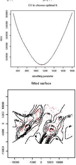
We have plottedCV(h), as given by Equation (5), in Fig. 4. There is a unique minimum at h=1124 (which
corresponds to a RMSE value of
CV(1124) / n=69.69) and this value of h is then used in Equation (2) to estimate the rainfall over a grid of values. A contour plot of the predicted rainfall is shown in Fig. 4. As expected, it can be seen that there is broad agreement between the y values and the fitted values.
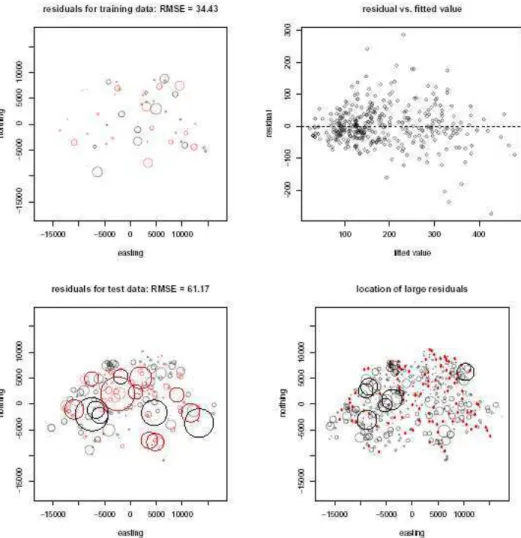
The fitted model, in which m(x)ˆ is estimated from the training data, can be used to obtain fitted values for the training data and to predict the test data. As expected, the RMSE is much reduced (from 69.69 to 34.43) when the training data is simply resubstituted, but the RMSE from the test data is 61.17, which is very similar to the minimized CV estimate. Fig. 5 shows the residuals from the fitted model, the locations of the larger residuals and how the residuals are related to the predicted values for the test data.
L2BOOSTING
Introduction: L2Boosting stagewisely optimizes the squared loss function(m m) / 2− ˆ 2 . Specifically, it is a
procedure of iterative residual fitting where the final output is simply the sum of the fits. Formally, consider
a weak learner. m ;S,ˆ
(
⋅ γ)
, that in the L2Boosting terminology is simply a crude smoother. An initial leastb
ˆ
m ( )⋅ is the sum of mˆb 1− ( )⋅ and a least
Fig. 4: Cross-validation function of residual sum of squared errors, which gives optimal value of h=1124 and resulting trend surface contour plot, of the N-W estimator. The original data are shown as circles with size corresponding to the rainfall.
squares fit of the residuals
e i i i ˆb 1 i
S ={X , e = −Y m − (X )}, i.e. m ;S ,ˆ
(
⋅ e γb)
. The L2Boosting estimator ism ( )ˆB ⋅ .The two main issues are the bandwidth selection and the choice of the number of boosting iterations B . As the end is to get a weak learner, a natural and direct way for reducing the complexity of whatever kernel method is oversmoothing. This is because large values of the bandwidth reduce the locality of the method and consequently, overfitting. Thus the smoothing parameter can be viewed as a potential component of regularization. A quite similar point of view is supported by Vapnik[4] (pp. 327-330) who upholds that in kernel density methods regularization can be achieved by modifying the window width. This is
“makes robust” problems whose solutions have big changes for small changes in data, as kernel smoothing is considered. From this perspective we can well understand that big bandwidths regularize the learning process.
We propose to boost the N-W estimator in an obvious L2Boosting manner. Our boosting algorithm is described by the following pseudocode:
Algorithm:L2boostNW
(Initialization) Given S and h>0 , calculate mˆ1
( )
x =mˆNW(
x;S, h)
. (Iteration) Repeat for b=2,..., Bcompute the residualsei =Yi−mˆb 1−
( )
Xi i=1,..., n; update mˆb( )
x =mˆb 1−( )
x +mˆNW(
x;S , he)
, wheree i i
S ={(X , e ),i=1,…, n} .
Note that our choice of using a fixed smoothing parameter along the iterations seems appropriate. In fact, if we optimally select the smoothing parameter for every estimation task, we would encourage the overfitting tendency, since the “learning rate” of every single step is maximized. However a formal justification is presented later, in which small bias properties are proved to hold when the bandwidth is fixed over boosting iterations.
L2boostNW reduces the bias of the N-W estimator:
Here, we will show (for the univariate case, d=1 ) how boosting reduces the asymptotic bias, up to boundary effects, of the N-W estimator. The result clearly extends to d≥2 by considering multivariate Taylor series' expansions.
Assume conditions (a)-(e) hold, after the first boosting step we have
( )
( )
( )
( )
( )
i i i i ix X x X
n n
i i
i 1 h i 1 h
2 n x X n x X
i 1 h i 1 h
x X n 1 0 i i 1 nh h
K Y K e
ˆ m (x)
K K
ˆ ˆ
2r(x) K m (X )
. ˆf(x) − − = = − − = = − = = + − =
∑
∑
∑
∑
∑
We take the expectation of the numerator and denominator as before. We already have Er(x)
⌢
from Equation (3) and Ef (x)
⌢
from equation (4). So the only thing we need is the expectation of the second term in the numerator. By ignoring the non-stochastic term (when i=j ), expanding in a Taylor series and integrating, Di Marzio and Taylor[7] eventually obtain the following expression for the asymptotic expectation up to terms of order O(h )2
1
2 2
2 2
2
h 1 h f (x)
ˆ
m (x) r(x) m(x)f (x) 1
2 f (x) 2f (x)
µ µ −
′′ ′′ ≈ + + E 2 2 2 2 2 2
h f (x)
r(x) 2f
f (x) 2f h f (x) 2f h f (x)
As a consequence, we observe a reduction in the asymptotic bias from O(h2) to o(h2). This conclusion is consistent with that found by Di Marzio and Taylor[5,6], where boosting kernels gives higher order bias for both density estimation and classification. However, note that the current result uses L2Boosting for regression, rather than the Adaboost-like algorithms used in classification and density estimation. Remarkably, note that we have reduced the bias without requiring any new smoothness assumption. Although p-order polynomials smoothers become less biased when p increases, they require that at the same time the quantity
(p 1)
m + (x)exists.
Boosting the Swiss rainfall data predictions: We need to find the optimal pair (h, B) for our data and this can be done by leave-one-out cross-validation. Fig. 6 shows the estimates of RMSE for various values of B and h. The optimal value was found for B=2 and h=1269.4, which gave a resulting CV estimate of RMSE of 69.244. This is only a very small improvement on B=1 (no boosting). Using the pair (1269.4, 2) the RMSE on the test data was 60.99 which is a again a very small improvement on B=1 (61.17). The resulting trend surface of the boosted model is also shown in Fig. 6; it is very similar to that of Fig. 4.
COMPARISONS
Trend surface analysis: A standard method for the analysis of spatial data, is to fit a trend surface and then carry out kriging for predictions[22]. To be consistent with the previous approach we use cross-validation for parameter estimation and model selection. Firstly, we obtained the proper order of the fitted trend surface. The results are shown in Table 1 which indicates a quadratic (or possibly linear) model is optimal.
An assessment of the spatial structure was made by examining a correlogram (Fig. 7) of the residuals, which indicated that points close in space tended to be similar. Various models for the covariance function were fitted: gaussian, exponential and spherical. Using cross-validation based on the training data alone, it was found that the gaussian model was best (giving an estimated RMSE of 74.5 using leave-one-out CV on the training data).
Table 1: RMSE estimated by leave-one-out cross-validation of trend surface fitted by ordinary least squares
Surface order 0 1 2 3 4 5
RMSE 117.3 112.4 112.0 115.1 115.5 112.4
The gaussian model was used to predict the test data, with a resulting RMSE of 72.66 and the fitted surface is shown in Fig. 7. Note that the fitted surface is
less smooth than that of the N-W estimator in Fig. 4, or of the boosted N-W estimator in Fig. 6.
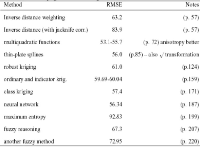
Other predictions: The edited volume Dubois et al.[11] contains many results from the original competition. Table 2 contains a summary. The kriging values given there are slightly better than we obtained and our N-W estimator (and its boosted version, in particular) performs reasonably well overall.
We note that the best combination of (h, B) (chosen with reference to the test data) is
h=2040.8, B=3 which gave RMSE=56.37 and so we might conclude that boosting N-W works reasonably well for this dataset.
Confidence intervals: Here, we consider confidence intervals for N-W estimates. In particular, we present two naive approaches and a paired bootstrap strategy discussed by Härdle[23]. We firstly discuss the naive approaches.
Table 2: Summary of results (RMSE values) from Dubois et al.[11],
with page numbers as given.
A totally naive method is to simply use Y±2×SD(Y)=(L, U)
(in which the mean and SD are estimated from the training data).
Using the kernel regression model we could simply use:
ˆ ˆ
m(x)±2σ =(L, U)
in which ˆσ is estimated by CV.
Fig. 5: Residuals from fitted model for the test data (top left) and dependence of the residuals on the fitted values (top right). The spatial structure of the residuals is also shown with gray-scale colors (bottom left) dependent on the sign and absolute size (bottom right).
Fig. 7: Left: Correlogram of residuals from fitted quadratic surface, with Gaussian covariance function fitted by eye. Right: Fitted trend surface by generalized least squares.
and these give fixed CI widths (U−L) of 466.7 and 278.7, respectively. Note that, although the coverage rate of these intervals is similar, the average width of the second naive method is much less.
A description of the naive bootstrap follows. Let
i i
{(x , y ), i∗ ∗ =1,…, n}be a sample, with replacement, from {(x , y ), ii i =1,…, n}. Taking B bootstrap samples of size n and forming a N-W estimate for each one at x, gives a population of B bootstrap estimates {m (x), bb∗ =1,…, B}. From these latter we can then obtain an empirical αth percentile as the value ˆt (x)α such that
B
b b 1
1 ˆ
I[m (x) t (x)]
B α α
∗
=
≤ =
∑
,where I[A] is the indicator of the event A, equal to 1 if A is true and 0 otherwise. Then, for any x, we could interpret (tˆα/ 2(x), tˆ1−α/ 2(x))as a (1−α)100% confidence interval for m(x) (interpolating as necessary for small B).
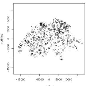
We have drawn 1000 bootstrap samples of size n=100 (with replacement) and got 248 counts, but with a quite low meansize of 140. Of the 119 which lie outside the confidence intervals, 71 are outside the lower interval and 48 are outside the upper interval. However, although 248/367 is only 68% (rather than 95%), note that the CIs are not simultaneous and those which are not in the CIs tend to be either clustered together, near the boundary, or are in regions where the density of test points is low; Fig. 8. However, the main cause of this rather poor coverage rate lies in the bias of the estimator. In particular, note that the above naive algorithm does not explicitly take into account accuracy when deriving the coverage rate. In fact, Hall[24] points out that the naive procedure is doomed to a poor
coverage rate because of the bootstrap estimator
Fig. 8: Test points which are inside 95% bootstrap confidence intervals (x) and outside (+). The dots indicate the training locations.
m (x)∗ is not centered on m(x) but on
ˆ ˆ
m(x)=m(x)+error(m(x)). Hall[25] argues that undersmoothing is preferable to an explicit bias estimation step as a strategy for improving the coverage rate. But undersmoothing worsens the point estimate. So the conclusion seems to be that the value of h optimal for the coverage rate differs from that one optimized for point estimation. Actually, if in our case study h is reduced to 450, then the coverage increases to 75% and the mean width increases to 164. However, the RMSE becomes 77 and further reductions in h lead to numerical instability in the N-W predictor.
the boosted estimate may yield improved coverage rates. In a similar manner to that described above, we can resample from the data and calculate a boosted N-W estimate of the test data using the bootstrap sample (a “boosted bootstrap”). In order to follow this approach, we have drawn 1000 bootstrap samples of size 50 and estimated by using, for every sample, the CV-optimzed values of (h, B). The resulting confidence intervals have coverage 337/367=92%, with an average width of 234 (searching a grid of h∈[300, 2400] and B in the range (1,2,3,4). So there is good evidence that higher order bias potentialities of boosting can be conveniently employed to improve the coverage rate.
CONCLUSIONS
The Swiss rainfall data are an extensively studied spatial dataset[11]. As seen, several approaches were employed to fit these data, both traditional and parametric like kriging and more recent nonparametric techniques. We have seen that locally adaptive techniques have been successfully employed for estimating the signal content of spatial data taken as a whole. This is additional evidence that a nonparametric analysis seems suitable for exploratory purposes in the selection stage of a parametric model as well as when the information on the specific case study does not allow parametric assumptions at all.
In this study we have proposed a new approach based on kernel smoothing and an adapted version of it by boosting. Our smoother was the popular N-W regression estimator with product kernels and cross-validated bandwidths. Quite interestingly, the N-W smoother has given very good performance, ranking among the methods with the best behavior. Moreover, its boosted version drastically improves on the construction of confidence intervals. Note that all of our results have been obtained with an automated approach using cross-validation and the selection of bandwidth and number of boosting steps has worked well. Overall, we should not draw conclusions from only one dataset, particularly given various user-inputs which can vary in a subjective manner and further simulations are necessary. However, our results confirm that confidence interval construction based on the N-W estimator is still an open and quite challenging problem.
REFERENCES
1. Michie, D., D. Spiegelhalter and C.C. Taylor, 1994. Machine Learning, Neural and Statistical Classification. Chichester. Ellis Horwood.
2. Shapire, R., 1990. The strength of weak learnability. Machine Learning, 5: 197-227. 3. Freund, Y., 1995. Boosting a weak learning
algorithm by majority. information and computation. Information and Computation, 121: 256-285.
4. Vapnik, V., 1998. Statistical Learning Theory. Wiley, London.
5. Di Marzio, M. and C.C. Taylor, 2004. Boosting kernel density estimates: a bias reduction technique? Biometrika, 91: 226-233.
6. Di Marzio, M. and C.C. Taylor, 2005. Kernel density classification and boosting: An L2 analysis. Statistics and Computing, 15: 113-123.
7. Di Marzio, M. and C.C. Taylor, 2006. Boosting kernel regression. (submitted).
8. Bühlmann, P. and B. Yu, 2003. Boosting with the l2 loss: regression and classification. J. Am. Stat. Assoc., 98: 324-339.
9. Friedman, J., T. Hastie and R. Tibshirani, 2000. Additive logistic regression: A statistical view of boosting. The Ann. of Stat., 28: 337-407.
10. Friedman, J., 2001. Greedy function approximation: A gradient boosting machine. The Ann. of Stat., 29: 1189-1232.
11. Dubois, G., J. Malczewski and M. De Cort (Eds.), 2003. Mapping radioactivity in the environment. Luxembourg: Office for the Official Publications of the European Communities.
12. Stein, M., 1999. Interpolation of Spatial Data. Some Theory for Kriging. Springer.
13. Yakowitz, S. and F. Szidarovsky, 1985. A comparison of kriging, with non-parametric regression methods. J. Multivariate Analysis, 16: 21-53.
14. Wahba, G., 1990. Spline Models for Observational Data. Philadelphia: Society for Industrial and Applied Mathematics.
15. Hutchinson, M.F. and F.R. Gessler, 1994. Spline-more than just a smooth interpolator. Geoderma, 62: 45-67.
16. Laslett, G.M., 1994. Kriging and splines: An empirical comparison of their predictive performance in some applications (with discussion). J. Am. Stat. Assoc., 89: 392-409. 17. Azari, A. and H.-G. Müller, 1992. Preaveraged
localized orthogonal polynomial estimators for surface smoothing and partial differentiation. J. Am. Stat. Assoc., 87: 1005-1017.
18. Høst, G., 1999. Kriging by local polynomials. Computational Statistics and Data Analysis, 29: 295-312. 19. Altman, N., 2000. Krige, smooth, both or neither?
(with discussion). Australian and New Zealand J. Stat., 42: 441-461.
20. Opsomer, J., D. Ruppert, M. Wand, U. Holst and O. H¨ossier, 1999. Kriging with nonparametric variance function estimation. Biometrics, 55: 704-710. 21. Fan, J. and I. Gijbels, 1996. Local Polynomial
Modelling and its Applications. Chapman & Hall, London.
22. Ripley, B.D., 1981. Spatial Statistics. New York: Wiley. 23. Härdle, W., 1990. Applied Nonparametric
Regression. Cambridge University Press.
24. Hall, P., 1992a. The Bootstrap and Edgeworth Expansion. Springer, New York.