Estud. Econ. vol.39 número3

 Alex luiz FerreirA  roselidA silvA

Resumo

O objetivo deste artigo é investigar as causas gerais dos diferenciais da taxa de juros real (rids) para um conjunto de países emergentes, para o período de janeiro de 1996 a agosto de 2007. Para tanto, duas metodologias são aplicadas. A primeira consiste em decompor a variância dos rids entre a paridade do poder de compra relativa e a paridade de juros a descoberto e mostra que os diferenciais de inflação são a fonte predominante da variabilidade dos rids; a segunda decompõe os rids e os diferenciais de juros nomi-nais (nids) em choques nominomi-nais e reais. Sob certas condições de identificação, modelos autorregressivos bivariados são estimados com tratamento adequado para as quebras estruturais identificadas e as funções de resposta ao impulso e a decomposição da variância dos erros de previsão são obtidas, resultando em evidências favoráveis a que os choques reais são a causa mais provável dos rids.

PalavRas-Chave

diferencial de juros reais, países emergentes, quebras estruturais, decomposição da variância dos erros de previsão

abstRaCt

The aim of this paper is to investigate the general causes of real interest rate differentials (rids) for a sample of emerging markets for the period of January 1996 to August 2007. To this end, two methods are applied. The first consists of breaking the variance of rids down into relative purchasing power pariety and uncovered interest rate parity and shows that inflation differentials are the main source of rids variation; while the second method breaks down the rids and nominal interest rate differentials (nids) into nominal and real shocks. Bivariate autoregressive models are estimated under particular identification conditions, having been adequately treated for the identified structural breaks. Impulse response functions and error variance decomposition result in real shocks as being the likely cause of rids.

KeywoRds

real interest rate differentials, emerging markets, structural breaks, breakdown of prediction errors vari-ance

Jel ClassifiCation

F32, F36, F21

 _{Departamento de Economia, FEA-RP/USP. Endereço para contato: Av. Bandeirantes, 3900 – Ribeirão Preto – SP. CEP:} 14040-900. E-mail: alexferreira@usp.br.

 _{Departamento de Economia, FEA-RP/USP. Endereço para contato: Av. Bandeirantes, 3900 – Ribeirão Preto – SP.} CEP: 14040-900. E-mail: roselisilva@fearp.usp.br.

1 IntRoDuctIon

Uncovered Interest Rate Parity (UIP) with rational expectations and relative Purchasing Power Parity (PPP) entail the Real Interest Rate Parity Hypothesis (RIPH) [Roll (1979)]. The common finding regarding the existence of ex post real interest rate differentials (rids, hereafter) across countries since the seminal papers of Mishkin (1984) and Cumby and Obstfeld (1984) is that rids are autoregres-sive and relatively short-lived (see, for instance, ObsTfeld; TaylOR, 2003 and GOldbeRG et al., 2003). The aim of the current paper is to investigate the general causes of rids. for this purpose, we use a selected sample of emerging markets in which latest evidence indicated that rids (in relation to the Usa) mean-revert to a positive equilibrium (see feRReIRa; león-ledesMa, 2007).

departures from RIPH can be explained by ex post deviations from PPP and UIP. Hence, a question that arises is whether rids are caused by frictions in goods or as-sets markets? another interrelated question is if real shocks (changes in risk percep-tion or productivity increases, for example) are more important than nominal shocks (such as unexpected changes in money supply, for instance) to explain deviations from interest parity. These questions are relevant because RIPH is based on the existence of frictionless markets and rids reflect the degree of market integration. The answers might be of practical importance for researchers as well as for policy makers. for example, stabilising the variance of rids can be a target of monetary policy in itself.1 _{If rids are very volatile, returns are unstable and investors dislike}

variance. The higher the variance, the smaller is the incentive to invest in a bond and the greater must be its return. Hence, policy makers may want to offset shocks that cause great variability. also, high rids can impose heavy costs to an economy − because of interest payments on the public, domestic and foreign debt − so unveiling the causes and understanding their dynamics is essential to design the appropriate macroeconomic policies to change differentials. finally, the long-run money neutral-ity is still a motivating question, which is tested in an innovative way.

There are also theoretical issues motivating the work. Variance decompositions can shed light on the nature of the relationship between rids and real exchange rates. There has been a debate on whether this relationship holds since frankel (1979). evidence can be non-supportive as Meese and Rogoff (1988), edison and Pauls (1993), Macdonald (1998), breedon et al. (1999) and Isaac and de Mel (2001) or favourable as astley and Garrat (2000), Chortareas and driver (2001), Macdonald and nagayasu (2000), Camarero and Tamarit (2002) and Jin (2003). because of balassa-samuelson effects, the sign of an impact of a real shock on exchange rates

(and rids, as we will explain) is undetermined and depends on the type of the dis-turbance and the sector of the economy that is hit. The proposed tests can help to clarify this issue − as observed by Macdonald and Ricci (2004) − rids might capture productivity differentials.

We focus on the importance of the international parity conditions on the determina-tion of rids. The broad quesdetermina-tion is whether rids can be explained by ex post deviadetermina-tions from PPP and UIP and to which extent. The main objective is to separate out the driving sources of volatility in the variance of rids. The second goal of the paper is to characterise the dynamic response of rids to real and nominal disturbances and to breakdown its variability according to these two types of shocks.

The paper presents further evidence on a higher degree of friction in assets rather than goods’ markets and the predominance of real shocks in the path of rids for a set of emerging economies. To our knowledge, no work has performed innovation accounting on rids, hence the tests are innovative in this sense. The work also com-plements papers on the relationship of real exchange rates and rids by reinforcing the finding of no correlation between variables. The rest of the paper is organised as follows. section 2 describes the methodology involved in the tests and discusses the identifying restrictions; section 3 explains the data and presents the results. section 4 concludes.

2 MEtHoDology anD tHEoRy

The first method draws insights from levine (1991) and frankel and Macarthur (1988) but it is based on Cheung et al. (2003). The latter has separated the variance of rids between deviations from relative PPP and UIP using the relationships given by RIPH as in the following equation

* *

( e) ( e)

t t t t t t t

rid = i − − ∆i s − π − π − ∆s (1)

where rid is the real interest rate differential, i is the domestic nominal interest rate and i* is the foreign interest rate that matures at time t. The nominal exchange rate, s, is the domestic price of the foreign currency; the expected rate of depreciation is

1

1

e e t t

t

S

s

S

∆ =

−

standing for time. domestic and foreign rates of inflation are πtand

*

t

respecti-vely. Observe that it− − ∆it* steare ex ante deviations from UIP and

* e

t t st π − π − ∆

correspond to ex ante deviations from PPP.

Given the definition of variance and covariance and noting that forecast errors cancel out in (1), we can write

* * * *

Var(ridt)=Var(it− − ∆ +it st) Var(π − π − ∆ −t t st) 2 Cov(it− − ∆ π − π − ∆it st, t t st) (2)

another way to decompose the variance of rids is by noting that changes in the exchange rate also cancel out in (1). as rids are equal to interest rate differentials subtracted from inflation differentials by construction, we can also write

* * * *

Var(

rid

)

=

Var(

i

−

i

)

+

Var(

π − π −

)

2 Cov(

i

− π − π

i

,

)

as explained by engel (1996, p. 138), this type of RIPH decomposition “makes sense – real interest parity could fail either because ex ante PPP fails (goods markets are not integrated) or because uncovered interest parity fails (capital markets are not integrated)”. engel (1996) has further criticised the works of Canova (1991), bekaert (1994), Gokey (1994) and Huang (1990) who decomposed deviations from UIP into devia-tions from PPP and RIPH because “Efficiency of the forward market does not require ex ante PPP or ex ante real interest equality. Both could fail, and fail wildly, yet uncovered interest parity could still hold.” (p. 137). apart from Cheung et al. (2003), the only work performing variance decomposition along the lines set on (2) and (3) is Tanner (1998). However, Tanner’s (1998) paper suffers from the same shortcomings raised by engel (1996) to the aforementioned previous works. The reason is that Tanner (1998) decomposes both the level and the variance of UIP deviations between

de-viations from PPP and RIPH.2

The second method consists in recovering the relevant parameters for innovation accounting using short and long run restrictions on a bivariate VaR system of equa-tions. In this part of the paper, we base our tests on the methodology employed by enders and lee (1997). These authors first ran a VaR using real and nominal exchange rate variations as dependents variables and later applied the blanchard and Quah (1989) decomposition. They also presented a theoretical model that illustrates the impact of the two types of shocks, real and nominal, on exchange rates. The nominal shock has the property of not affecting the real variable on the long run while there is no restriction for the real shock. from rational expectations UIP,

2 His conclusion for the study for 34 emerging and developed economies is that the variance of rids

we know that there is a theoretical relationship between nominal exchange rate variations and nominal interest rate differentials. This relationship also occurs for real variables, which can be seen by subtracting inflation differentials from UIP as below

e

t t

rid = ∆q (4)

where e

t

q

∆ _{represents expected changes in the real exchange rate.. Hence, we can}

borrow the assumption that real and nominal factors are the disturbances affecting nominal interest rate differentials (nids, hereafter) and rids from the literature that applied variance decomposition to real exchange rates (see also ROGeRs, 1999, and asTley; GaRRaTT, 2000, for example) and write

11 12

0 0

( ) ( )

t t k t k

k k

rid c k r c k n

∞ ∞

− −

= =

=

∑

∑

21 22

0 0

( ) ( )

t t k t k

k k

nid c k r c k n

∞ ∞

− −

= =

=

∑

∑

where we ignored intercept terms for simplicity; real and nominal shocks are repre-sented by

ε ε

r

,

n

iid N(0,σ_ε) in which 2

ε

σ represents variance.

The letter c stands for the coefficients associated with the responses of rids and nids to shocks at each period k. The system of equations in (5) and (6) represent an infi-nite bivariate moving average (bMaR). a bMaR can be represented by a bivariate autoregression model (bVaR) if the roots of the lag polinomials are out of the unit circle, known as the invertibility conditions. The same condition applies to the lag polynomial of the bVaR which guarantees the stability conditions. Under such conditions, the bVaR representation is

1 1

11 12

21 22 1 2

( )

( )

( )

( )

t t t

t t t

rid

A L

A

L

rid

e

A

L

A

L

nid

nid

e

− −











 



=

+











 













 



where e1t and e2t stand for the error terms, which are composite of the pure

The Choleski decomposition imposes a contemporaneous restriction in (5) or (6) in order to recover their parameters from the estimates of the system in (7). The assumption is that a real shock does not have a contemporaneous impact on nids, a conjecture that is valid provided that real shocks affect prices instantaneously while interest rates are impacted after one lag.3 _{another interpretation is that policy}

mak-ers react to a real shock after having more knowledge of its nature. The time elapsed for the reaction to take place is one month.4

another alternative is the method proposed by blanchard and Quah (1989). for this decomposition we considered that the sum of nominal shocks has a zero impact on the series of rids

12 0

( ) t k 0

k

c k n ∞

− =

ε =

∑

following the idea of faust (1998), as explained below, the restriction in (8) is used to test for robustness of the Choleski decomposition as we cannot think about a theoretical explanation for (8) and recognise its contentious character.

as a matter of fact, either identifying restriction (long-run or contemporaneous) depends on a set of assumptions that might not be entirely accepted. It is often at-tributed to the bVaR literature, the use of implausible restrictions (assumptions) for identification. nonetheless, as pointed out by sims (1980), faust (1998) and faust et al. (2003), even incredible restrictions can result in useful analysis provided that reasonable economic interpretations can be given to the findings. faust (1998), for example, has elaborated a way of checking for robustness of contentious restrictions by taking a particular assumption and checking “…all possible identifications of the vaR for the one that is the worst case for the claim, subject to the restriction that the im-plied economic structure produce reasonable responses to policy shocks.” (p. 209, emphasis from the author). Then, he adds, “If in the worst case the variance share is small, then the claim is supported. If the share is large, then either the identifying information – the characterization of a reasonable policy shock – must be sharpened or we must view the is-sue as unsettled.” (p. 210). We performed and compared variance decompositions of rids using both short and long-run restrictions as a way to verify the “robustness” of the assumptions.

3 We discarded the possibility that a nominal shock does not contemporaneously affect rids because it is logically inconsistent. The reason is that a nominal shock would have to impact interest rates and prices both at the same time and by the same magnitude, leaving rids at time t absolutely unchanged. The inconsistency arises because even if there is no initial impact on rids, there would be lagged effects. 4 Monetary Policy Committee meetings in brazil, for example, are realised on a monthly basis and, in

3 REsults

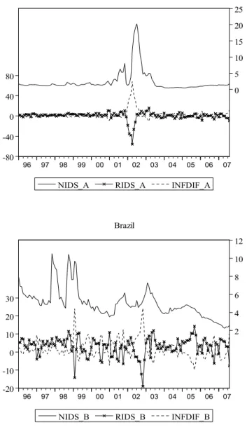
The emerging markets of the sample comprise the small open-economies of argentina, brazil, Chile, Mexico and Turkey. We used the Usa as the reference large economy for the calculation of the rid. The period of the tests corresponds to the interval that spans from 1996M1 to 2007M8.

The sample period starts in the mid 90s because harmonised data for the construc-tion of rids for some countries did not exist before this period and also because after the mid-90s most of the countries had liberalised capital markets and had ad-vanced substantially in their trade liberalisation process. In addition, this period is characterised by various shocks from financial crises: asian, Russian, brazilian and argentinean. The higher volatility that followed these crises justifies the choice for the variance decomposition and innovation accounting. data on interest rates and average exchange rates was obtained from IMf’s International financial statistics (Ifs). We have chosen the Treasury bill Rate for brazil and Mexico while deposit rates for argentina, Chile and Turkey because of data availability. The inflation rate is either the rate of growth of the Producer Price Index (PPI) or the Wholesale Price Index (WPI), which are more sensitive to variations in the price of trada-bles. We transformed the annualised monthly interest rate and the inflation rate into compounded quarterly rates and then subtracted the latter from the former. Quarterly exchange rate changes were calculated using the average of the corres-ponding period.

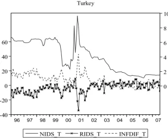
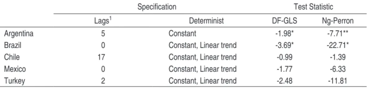
FIguRE 1 – RIDs, nIDs anD InFlatIon DIFFEREntIals (InFDIF)

-80 -40 0 40 80

0 5 10 15 20 25

96 97 98 99 00 01 02 03 04 05 06 07

NIDS_A RIDS_A INFDIF_A Argentina

-20 -10 0 10 20 30

2 4 6 8 10 12

96 97 98 99 00 01 02 03 04 05 06 07

-10 -5 0 5 10 15

0 1 2 3 4 5 6

96 97 98 99 00 01 02 03 04 05 06 07

NIDS_C RIDS_C INFDIF_C Chile

-8 -4 0 4 8 12

0 2 4 6 8 10 12

96 97 98 99 00 01 02 03 04 05 06 07

-40 -20 0 20 40 60

0 2 4 6 8 10

96 97 98 99 00 01 02 03 04 05 06 07

NIDS_T RIDS_T INFDIF_T Turkey

taBlE 1 – soME DEscRIPtIvE statIstIcs oF RIDs anD nIDs

Variable Mean Min Max Std. Dev.

Argentina nids 2.34 0.44 20.28 3.29

rids _{0.31 -55.96 15.93 8.18}

Brazil nids 5.01 2.24 10.52 1.62

rids _{2.98 -18.98 14.30 5.05}

Chile nids 1.53 0.30 5.92 1.09

rids _{0.74 -8.31 10.75 4.07}

Mexico nids 3.38 1.04 10.30 2.22

rids 1.70 -7.10 9.48 2.83

Turkey nids 4.04 1.11 9.64 2.12

rids _{-3.55 -34.56 9.21 6.87}

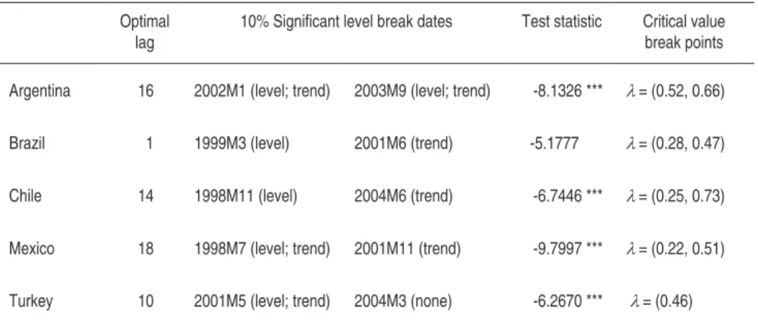
In order to find out the order of integration of nids before running the bVaR, we initially tested for the presence of unit roots.5 Considering the low power prob-lems and size distortions of the traditional tests (augmented dickey-fuller - adf, Phillips-Perron - PP - and Kwiatkowski, Phillips, schmidt and shin - KPss), large-ly pointed in the literature6_{, we applied more robust tests such as the df-Gls}

(ellIOT et al, 1996 and ellIOTT, 1999) and ng-Perron (1996, 2001) tests.

5 We have not performed unit root tests for rids as this has already been done for the countries of our sample, see for example ferreira and león-ledesma (2007). as pointed out earlier, results show that this variable is stationary.

We first apply df-Gls (ellIOTT; ROTHenbeRG; sTOCK, 1996) who pro-pose a simple modification to the adf, in which the time series is previously filtered from its deterministic components. The first set of tests, which goes along the lines of the adf, allows for an adequate analysis of the series in the presence of deter-ministic components.

The second test, proposed by ng and Perron (1996, 2001), follows the non-para-metric methodology of the PP tests, in which the variance-covariance matrix of the parameters from the test equation is robust to heteroscedasticity and autocorrela-tion. The authors propose to treat the problems associated with the usual tests by building a test statistic without the deterministic components (the latter estimated by Gls) and spectral density function at zero frequency estimated as an aR(1) process (PeRROn; nG, 1998).

We found the optimal augmentation lag using a Modified akaike information Criterion (MaIC), following ng-Perron (2001). We report the deterministic com-ponents, lag specification, t-ratios, and critical values for df-Gls and ng-Perron tests in Table 2.

taBlE 2 – unIt Root tEsts on nIDs

Speciication Test Statistic

Lags1 _{Determinist DF-GLS Ng-Perron}

Argentina 5 Constant -1.98* -7.71**

Brazil 0 Constant, Linear trend -3.69* -22.71*

Chile 17 Constant, Linear trend -0.99 -1.39

Mexico 0 Constant, Linear trend -1.77 -6.33

Turkey 2 Constant, Linear trend -2.48 -11.81

notes: 1 starting from 13 lags (except Chile, 24), MaIC selection.

* Rejection of the null at 5% (** at 10%) confidence level.

we performed unit root tests that account for two possible structural breaks: the lee and strazicich (2003)test, ls test hereafter.

The advantage of the ls test, besides the endogenous investigation of two possible breaks, is to specify a test with breaks on both the null and the alternative which does not leave any ambiguity regarding the trend in the series: the rejection of the null implies a trend-stationary series. suppose the following data generation process:

t t t

nid

= d

′

Z

+

e

1

t t t

e

= β

e

+ ε

Where Zt is a vector of exogenous variables and

(

)

2

~ 0,

t iid N

ε σ _, d is a vector of

parameters. Model a (crash model) allows for two breaks in level, including two dummies D1td and D2t, so Z_t =

[

]

0 otherwise, and model C includes two breaks in level and trend, a changing growth model where Zt = 1, ,t D1t,D2t,DT1t,DT2t where DTjt =1for t≥TBj+1, j=1, 2, and 0

otherwise. The results are reported in Table 3.

taBlE 3 – nIDs: two-BR Eak MInIMuM lM unIt Root tEst (ls tEst)

Optimal lag

10% Signiicant level break dates Test statistic Critical value break points

Argentina 16 2002M1 (level; trend) 2003M9 (level; trend) -8.1326 *** λ = (0.52, 0.66)

Brazil 1 1999M3 (level) 2001M6 (trend) -5.1777 λ = (0.28, 0.47)

Chile 14 1998M11 (level) 2004M6 (trend) -6.7446 *** λ = (0.25, 0.73)

Mexico 18 1998M7 (level; trend) 2001M11 (trend) -9.7997 *** λ = (0.22, 0.51)

Turkey 10 2001M5 (level; trend) 2004M3 (none) -6.2670 *** λ = (0.46)

Obs: critical values are shown below for the one and two-break minimum lM unit root test with linear trend (Model C) at the 1%, 5%, and 10% levels for a sample of size T ¼ 100, respectively.

Critical values are symmetric around λ and (1 - λ), where λi = Tbi/T and can be interpolate at additional break points.

notes: *, **, *** significant at the 10%, 5%, and 1% levels, respectively.

Obs: the critical values shown below come from Table 2 in lee and strazicich (2003) for two breaks and from strazicich et al. (2004) for one break.

Two-breaks critical values

One-break critical values

1% 5% 10% 1% 5% 10%

λ = (0.2, 0.4) -6.16 -5.59 -5.27 λ = (0.4) -5.05 -4.50 -4.18

λ = (0.2, 0.6) -6.41 -5.74 -5.32 λ = (0.5) -5.11 -4.51 -4.17

λ = (0.2, 0.8) -6.33 -5.71 -5.33

λ = (0.4, 0.6) -6.45 -5.67 -5.31

λ = (0.4, 0.8) -6.42 -5.65 -5.32

λ = (0.6, 0.8) -6.32 -5.73 -5.32

taBlE 4 – vaRIancE DEcoMPosItIon oF RIDs BEtwEEn uIP anD PPP DEvIatIons

Argentina Brazil Chile Mexico Turkey

Variance of:

Rids 66.9 25.5 16.6 8.0 47.2

Deviations from UIP 306.5 98.4 19.6 14.5 122.3

Deviations from PPP 122.4 68.7 14.4 17.2 72.6

% of Rids’ variance:

Deviations from UIP 458.3 386.4 118.1 180.8 259.3

Deviations from PPP 183.0 269.8 87.2 215.3 153.9

-2cov(UIP,PPP) -537.5 -552.2 -104.6 -293.9 -311.0

The high volatility of exchange rates is responsible for most part of the variance of the individual parity conditions. a clear picture on the causes of deviations from RIPH emerges when rids are decomposed between nids and inflation differentials, as in Table 5. It becomes apparent that inflation differentials are the predominant source of variability for most rids of the sample. The variance of nids is higher during the period of the financial crises during the 1990s. after the nineties they are much more stable and, for this reason, the variance of the inflation differential dominates the series.

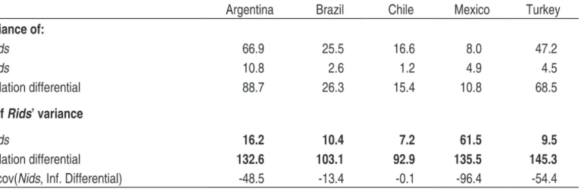
taBlE 5 – vaRIancE DEcoMPosItIon oF RIDs BEtwEEn nIDs anD InFlatIon DIFFEREntIals

Argentina Brazil Chile Mexico Turkey

Variance of:

Rids 66.9 25.5 16.6 8.0 47.2

Nids _{10.8 2.6 1.2 4.9 4.5}

Inlation differential 88.7 26.3 15.4 10.8 68.5

% of Rids’ variance

Nids 16.2 10.4 7.2 61.5 9.5

Inlation differential 132.6 103.1 92.9 135.5 145.3

The covariance between nids and inflation differentials and the value of the corre-lations (the latter is not reported) indicate that the two variables have some degree of dependence. In conclusion, the volatility of inflation differentials explains rids’ variance.

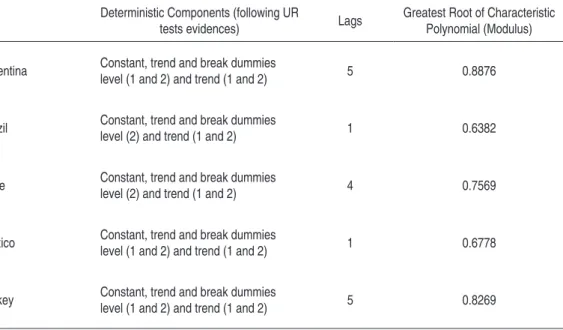
We turn to the findings of innovation accounting by first analysing forecast error variance decompositions. for this purpose, we estimated a bVaR for each country according to equation (7). However, the results of trend-stationary nids indicated that there are deterministic trend components, although with breaks (Tables 2 and 3), which must be taken into account in order to guarantee a stable bVaR. as we are interested in decomposing the error variance of the bVaR, we need to specify it in a way that errors are white-noise with the stationarity conditions met. Table 6 summarise the results.

taBlE 6 – BvaR sPEcIFIcatIon

Deterministic Components (following UR

tests evidences) Lags

Greatest Root of Characteristic Polynomial (Modulus)

Argentina Constant, trend and break dummies

level (1 and 2) and trend (1 and 2) 5 0.8876

Brazil Constant, trend and break dummies

level (2) and trend (1 and 2) 1 0.6382

Chile Constant, trend and break dummies

level (2) and trend (1 and 2) 4 0.7569

Mexico Constant, trend and break dummies

level (1 and 2) and trend (1 and 2) 1 0.6778

Turkey Constant, trend and break dummies

level (1 and 2) and trend (1 and 2) 5 0.8269

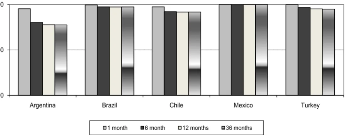
FIguRE 2 – FoREcast ERRoR vaRIancE DEcoMPosItIon oF RIDs

0 50 100

Argentina Brazil Chile Mexico Turkey

Percent of Forecast Error Variance Accounted for Real Shocks

1 month 6 month 12 months 36 months

note: The forecast error variance decomposition is the percentage of the mean squared error due to a real shock.

figure 3 presents impulse responses obtained through the use of Choleski technique as short-run responses would be somewhat influenced by the lagged restriction. long run restrictions leave the short run dynamics of the bVaR unconstrained or data-determined and structural theoretical explanations for variance decompositions and impulse responses can be made, as Clarida and Gali (1994) and astley and Garratt (2000) emphasised.

BR aZIl

MExIco

tuRkEy

rise generates an unexpected appreciation. The channel by which risk affects rids is direct. Hence, an unanticipated increase in risk raises rids. finally, a real demand shock leads to a permanent real appreciation and also enlarge rids.

Responses were normalised so each structural shock correspond to one standard deviation. as can be seen in figure 3, both rids and nids of argentina react in a similar way to either a real or a nominal shock. The oscillation pattern is the same for both rids and nids. a nominal shock has an initial positive impact (until the 5th period) over nids while the real shock has a negative impact. The response of argentinean rids and nids to nominal and real shocks follow the same pattern, with positive effects until the 5th period and a change of signs every five periods (approximately).

The behaviour of the impulse response function for Turkey is similar to the one of argentina. It oscillates and the convergence is slow, which is a result of a longer short run dynamics (both Turkey and argentina were found to have 5 optimal aug-mentation lags, see Table 6). However, this is the only country in which nids respond positively to a real shock, which occurs from the second lag onwards.

Impulse response for brazil and Mexico converge exponentially. This result is in accordance to its short-run dynamics, which presents one lag. nids respond to a real shock negatively and converge to zero from the third period onwards. Chile has a more complex short-run dynamics, (the optimal augmentation lag is 4) and presents an undershooting of both nids and rids in response to a nominal shock.

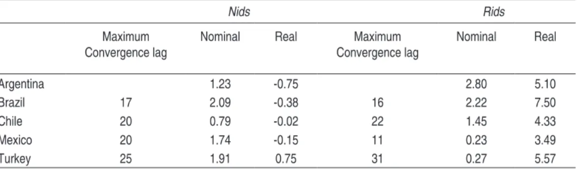
taBlE 7 – accuMulatED IMPulsE REsPonsE FunctIons

Nids Rids

Maximum Convergence lag

Nominal Real Maximum Convergence lag

Nominal Real

Argentina 1.23 -0.75 2.80 5.10

Brazil 17 2.09 -0.38 16 2.22 7.50

Chile 20 0.79 -0.02 22 1.45 4.33

Mexico 20 1.74 -0.15 11 0.23 3.49

Turkey 25 1.91 0.75 31 0.27 5.57

finally, while the sign of the accumulated impact of real shocks on nids is negative on average, they are positive for rids of all countries. as the 1990’s was a period characterised for productivity increases, this result, prima facie, lends support for balassa-samuelson effects.7 _{However, the 1990’s was also plagued by financial crisis}

which possibly imply risk premium shocks.

4 concluDIng REMaRks

deviations from international parity conditions do not provide a clear picture on the causes of rids because exchange rate changes are very volatile and, in fact, cancel out in the composition of rids. The variance of inflation differentials explains most part of the volatility of rids for all countries. Recall that rids are calculated ex post so the aforementioned variance decomposition does not require any statistical test based on probabilities because rids are equal to nids subtracted from inflation differentials by definition.

We found evidence of trend-stationarity for most nids in our sample. forecast error variance decomposition shows that real shocks explain most part of the variation in rids and the results are robust to either form of identifying restriction. The effect of a real shock tends to be amplified in the long run, reflecting the fact that, whenever differentials of developing economies start to grow, the tendency is for them to ac-cumulate by more than the initial increase. This reinforces the findings of frictions in assets markets. The sign of the accumulated impact of a real shocks on nids is negative while it is positive for rids of all countries. at the extent to which real

cks reflect productivity changes, this result provides support for balassa-samuelson effects. However, the 1990s was a period of various financial crises and the results of endogenous date breaks seem to reflect this fact. finally, nominal shocks impact positively on rids and nids in the long-run.

arbitrage is supposed to be largely enforced by increased market integration. as the sample period follows the trade and financial liberalisation, one would expect that departures from parity conditions played a minor role in the composition of rids. This possibility is weakened if imperfect asset substitutability is a plausible conjec-ture for the financial markets. The findings of the present paper reveal the predo-minance of real shocks in the path of rids and points out to deviations from UIP as their driving source. nids were found to be trend stationary, probably reflecting the tendency in reduction following the financial crises in the 1900s. The conclusion is that one should look at unexpected productivity changes and risk premium shocks in order to comprehend the dynamic behaviour of real differences in returns across countries.

REFEREncEs

asTley, M. s.; GaRRaT, a. exchange rates and prices: sources of sterling real

exchange rate fluctuations 1974-94. oxford Bulletin of Economics and statistics,

62, p. 491-509, 2000.

beKaeRT, G. exchange rate volatility and deviations from unbiasedness in a

cash-in-advance model. Journal of International Economics, 36, p. 29-52, 1994.

beVeRIdGe, s.; nelsOn, C. R. a new approach to decomposition of economic time series into permanent and transitory components with particular attention

to measure of the ‘business cycle’. Journal of Monetary Economics, 7, p. 151-174,

1981.

blanCHaRd, O. J.; QUaH, d. The dynamic effects of aggregate demand and

supply disturbances. american Economic Review, 79, p. 655-673, 1989.

bReedOn, f., HenRy, b.; WIllIans, G. long-term real interest rates:

evi-dence on the global capital market. oxford Review of Economic Policy, v. 15, n.

2, p.128-142, 1999.

CaMaReRO, M.; TaMaRIT, C. a panel cointegration approach to the

estima-tion of the Peseta real exchange rate. Journal of Macroeconomics, v. 24, n. 3, p.

371-393, 2002.

CanOVa, f. an empirical analysis of ex ante profits from forward speculation in

foreign exchange markets. Review of Economics and statistics, 73, p. 489-496,

CHeUnG, y-W.; CHInn, M.d.; fUJII, e. China, Hong Kong, and Taiwan: a

quantitative assessment of real and financial integration. china Economic Review,

14, p. 281-303, 2003.

CHORTaReas, G. e.; dRIVeR, R. l. PPP and the real exchange rate-real interest rate differential puzzle revisited: evidence from nonstationary panel data. bank

of england, working Paper series n. 138, p. 1-29, 2001.

ClaRIda, R.; GalI, J. sources of real exchange rate fluctuations: how important are nominal shocks?, carnegie-Rochester conference series on Public Policy, elsevier, 41, p. 1-56, 1994.

CUMby, R.; ObsTfeld, M. International interest rate and price level linkages under flexible exchange rates: a review of recent evidence. In: bIlsOn, J.;

MaRsTOn, R. C., (ed.). Exchange rate theory and practice. Chicago: University

of Chicago Press, 1984.

edIsOn, H. J.; PaUls, b. d. a re-assessment of the relationship between real

ex-change rates and real interest rates: 1974-1990. Journal of Monetary Economics,

31, p.165-187, 1993.

ellIOTT, G. efficient tests for a unit root when the initial observation is drawn

from its unconditional distribution. International Economic Review, 40, p.

767-783, 1999.

______; ROTHenbeRG, T. J.; sTOCK, J.H. efficient tests for an autoregressive

unit root. Econometrica, 64, p. 813-836, 1996.

endeRs, W.; lee, b.-s. accounting for real and nominal exchange rate movements

in the post-bretton Woods period. Journal of International Money and finance,

16, p. 233-254, 1997.

enGel, C. The forward discount anomaly and the risk premium: a survey of recent

evidence. Journal of Empirical Finance, 3, p. 123-191, 1996.

faRIa, J. R.; leOn-ledesMa, M. a. Testing the balassa–samuelson effect:

implications for growth and the PPP. Journal of Macroeconomics, v. 25, n. 2, p.

241-253, 2003.

faUsT, J. The robustness of identified var conclusions about money.

carnegie-Rochester conference series on Public Policy,49, p. 207-244, 1998.

______; ROGeRs, J. H.; sWansOn, e.; WRIGHT, J. H. Identifying the effects of

monetary policy shocks on exchange rates using high frequency data. Journal of

the European Economic association, MIT Press, v. 1, n. 5, p. 1031-1057, 2003.

feRReIRa, a. l.; león-ledesMa, M. a. does the real interest parity hypothesis

hold? evidence for developed and emerging economies. Journal of International

Money and Finance, v. 26, n. 3, p. 364-382, 2007.

fRanKel, J. a. On the Mark: a theory of floating exchange rates based on real

inter-est differentials. the american Economic Review, v. 69, n. 4, p. 610-622, 1979.

GOKey, T. C. What explains the risk premium in foreign exchange returns? Journal

of International Money and Finance,13, p. 729-738, 1994.

GOldbeRG, l.G.; lOTHIan, J.R.; OKUneV, J. Has international financial

integration increased? open Economies Review, 14, p. 299-317, 2003.

HUanG, R. d. Risk and parity in purchasing power. Journal of Money, credit and

Banking 22, p. 338-356, 1990.

IsaaC, a. G.; de Mel, s. The real-interest-differential model after 20 years. Journal

of International Money and Finance, 20, p.473-495, 2001.

IWaTa, s.; TanneR, e. Pick your poison: the exchange rate regime and capital

account volatility in emerging market. czech Journal of Economics and Finance,

v. 57, Issue7-8, p. 363-381, 2007.

JIn, Z. The dynamics of real interest rates, real exchange rates and the balance of

pay-ments in China: 1980-2002. IMF working Paper wP/03/67, p. 1-27, 2003.

lee, J.; sTRaZICICH M. C. Minimum lagrange multiplier unit root test with two structural breaks. the Review of Economics and statistics, v. 85, n. 4, p. 1082-1089, 2003.

______.; TanG, M. K. does productivity growth lead to appreciation of the real

ex-change rate? Review of International Economics, v. 15, n. 1, p. 164-187, 2007.

leVIne, R. an empirical enquiry into the nature of the forward exchange rate bias. Journal of International Economics,30, p. 359-369, 1991.

MaCdOnald, R. What determines real exchange rates? The long and short of it. Journal of International Financial Markets, Institutions and Money, v. 8, issue 2, p. 117-153, 1998.

______.; naGayasU, J. The long-run relationship between real exchange rates and real interest rate differentials: a panel study. IMF staff Papers 47, 1, p. 116-128, 2000.

______.; RICCI, l. estimation of the equilibrium real exchange rate for south africa. south african Journal of Economics, v. 72, n. 2, p. 282-304, 2004.

Maddala, G.s.; KIM, I.M. Unit roots, cointegration and structural change. Cambridge: Cambridge University Press, 2003.

MCCallUM, b.T. a Reconsideration of the uncovered interest rate parity

hypoth-esis. Journal of Monetary Economics, v. 33, n. 1, p. 105-132, 1994.

Meese, R.; ROGOff, K. Was it real? The exchange rate-interest differential relation

over the modern floating-rate period. the Journal of Finance, v. 43, p. 933-948,

MIsHKIn, f. s. are real interest rates equal across countries? an empirical

inves-tigation of international parity conditions. the Journal of Finance, v. 39, n. 5,

p.1345-1357, 1984.

nG, s.; PeRROn, P. Useful modifications to some finite sample distributions

as-sociated with a first-order stochastic difference equation. Econometrica, 45, p.

463-485, 1996.

______. lag length selection and the construction of unit root tests with good size

and power. Econometrica, 69, p. 1519-1554, 2001.

ObsTfeld, M.; TalyOR, a. M. Globalization and capital markets. In: bORdO,

Michael d.; TaylOR, alan M.; WIllIaMsOn, Jeffrey G. (ed.). globalization

in Historical Perspective. University of Chicago Press, 2003.

PeRROn, P.; nG, s. an autoregressive spectral density estimator at frequency zero

for nonstationarity tests. Econometric theory, 14, p. 560-603, 1998.

ROGeRs, J. H. Monetary shocks and real exchange rates. Journal of International

Economics, 49, p. 269-288, 1999.

ROll, R. Violation of purchasing power and their implications for efficient

interna-tional commodity markets. In: saRnaT, M.; sZeGO, G. P. (ed.). International

finance and trade, 1. Cambridge, Mass.: ballinger, p.133-176, 1979.

sIMs, C. a. Macroeconomics and reality. Econometrica, v. 48, n. 1, p.1-48, 1980.

sTOCKMan, a. C. a theory of exchange rate determination. Journal of Political

Economy, v. 88, n. 4, p. 673-698, 1980.

______. Real exchange rate variability under pegged and floating nominal exchange

rate systems: an equilibrium theory. nBER working Paper 2565, 1988.

sTRaZICICH, M. C.; lee, J.; day, e. are incomes converging among OeCd

countries? Time series evidence with two structural breaks. Journal of

Macroeco-nomics, 26, p. 131–145, 2004.

TanneR, e. deviations from uncovered interest parity: a global guide to where the

action is. IMF working Paper wP/98/117, p. 1-24, 1998.

TaylOR, M. P. The economics of exchange rates. Journal of Economic literature, v.